Numerical simulation of the stress field in California:
implications for the stress perturbation by Big Bend
and Garlock Fault
Abstract: 2D finite element modelling is used to analyze the state of stress in and around the San Andreas Fault System (SAFS) taking the whole area of California. In this study we focus on the state of stress at the general seismogenic depth of 12 km, imposing elastic rheology. The purpose of the pres-ent study is to simulate the regional stress field and also to find the stress perturbation due to Big Bend and Garlock Fault. Although in nature there is lateral and vertical variation in rheology, our highly sim-plified domain properties have simulated results comparable with the observed data. Our imposed boundary condition (fixed North American plate, Pacific plate motion along N34W vector up to northern terminus of the San Andreas faults and N50E vector motion for the subducting Gorda plate) simulated the present day regional Hmax orientation and velocity vector. Simulated results show local effect on the stress field and displacement vector by the Big Bend and is further enhanced by the Garlock Fault, which may have significant impact on fault slip, stress, and hence deformation in the surrounding region.
Keywords:San Andreas Fault System (SAFS), 2D finite element modelling, Big Bend, Garlock Fault,
σHmax, velocity vector.
Simulation Tectonics Laboratory, Faculty of Science, University of the Ryukyus, Okinawa, 903-0213, Japan.
*e-mail: matrikakoirala@gmail.com M. P. KOIRALA*ANDD. HAYASHI
The San Andreas Fault System (SAFS), a complex sys-tem of faults that display predominantly large-scale strike slip displacement, is part of an even more com-plex system of faults, isolated segments of the East Pacific Rise, and scraps of plates lying east of the East Pacific Rise that collectively separate the North American plate from the Pacific plate (Wallace, 1990). The SAFS is mainly a right-lateral strike slip fault. It has many other small faults, some are left-lat-eral, some are thrusts and some normal faults. Present-day plate kinematics of the Pacific and North American plates reveals that the Pacific plate is mov-ing towards NW with respect to North American plate. The motion of the plate is approximately 3.4-6 cm a-1 on a N34W vector approximately (Atwater,
1970; Minster and Jordan, 1978; DeMets et al., 1994; Argus and Gordon, 2001; Savage et al., 2004; d’Alessio et al., 2005). At its north end, the San
Andreas Fault joins the Mendocino Fracture Zone at a high angle, and there the Gorda plate and Juan de Fuca plate are being subducted under the North American plate. The Juan de Fuca plate currently subducts under the North American plate with a gen-eralized vector motion of N50E (Swanson et al., 1989) and with a velocity of 3 cm a-1(Noson et al.,
1988). The Gorda plate subducts with a similar direc-tion, but at an average velocity of 1.8 cm a-1(Wood
we calculated the stress at the seismogenic crust (at 12 km depth) of the whole California area and tried to analyze the effect of the Big Bend and Garlock Fault on the stress field and displacement vector. For this, we use simple but powerful FE plain stress modelling.
The objectives of the present study are: 1) evaluate the state of stress along and around the SAFS, California; 2) deci-pher the stress perturbations due to the big bend and Garlock Fault on the SAFS; and 3) unravel the deflection in displacement vector by the Big Bend and Garlock Fault.
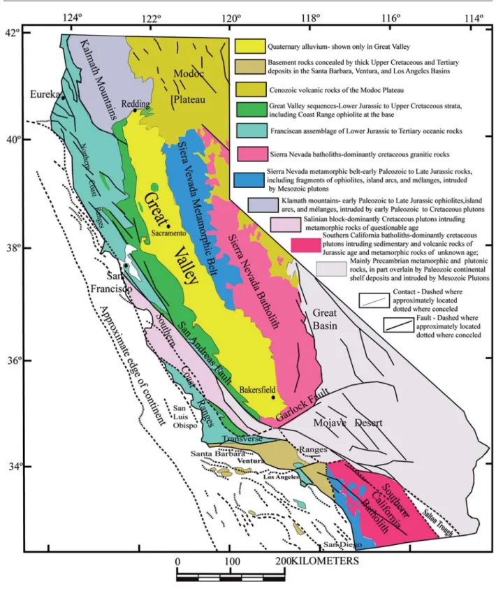
Elastic plane stress FE models are created to analyze the state of the stress on the whole California region, especially along and around the SAFS (Hayashi, 2008). Different domains are created in the model through variation of the domain properties. The sim-plified geological map of California modified after Irwin (1990) is taken as the base map (Fig. 1).
Model description
Models are created to analyze the state of stress along and around the SAFS. The simplified geological map of California (Fig. 1) is taken as the base map.
The FE software has been used in order to solve the elastic equations and for that we have to define the geometry of the models and the correct boundary conditions to apply to it. For the FEM calculation, the Young’s modulus (E), Poisson’s ratio (υ) and the density (ρ) are needed. The values selected are based on the available published literature (Bird and Kong, 1994; Cai and Wang, 2001; Chery et al., 2001; Lynch
and Richards, 2001; Malservisi et al., 2003; Parsons, 2006; Flesch et al. 2007).
Elastic behaviour of crust is assumed for the modelled area and this is justifiable since rheology changes from elastic to viscous at depths greater than 16 km depth in the study area (Fuis and Mooney, 1990). Recent studies of Becken et al.(2008) also show that the elas-tic (seismogenic) crust extends at least up to 12-15 km depth. Realistic boundary conditions have been applied to match the present-day plate kinematics in the Western North America and Pacific boundary.
Model geometry
The model covers the entire California area and con-sists of 1638 triangular elements and 879 nodes in plane stress condition. There are three types of models: (A) a first model consisting in whole California as a homogeneous one domain, (B) a second model with three domains (Pacific plate, North American plate and San Andreas Fault Zone), and (C) a third model
with four domains consisting of the Garlock Fault zone as fourth domain and the other three domains being the same as in the second model. The Fault zone boundary is made somewhat zigzag to mimic the actu-al fault geometry. Obviously, the width of the fault zone is slightly different at different places (Fig. 2).
Boundary condition
The boundary condition imposed represents the pres-ent-day plate kinematics of the Pacific plate, remnants of the Farallon plate and North American plate in the Western North America. In all models, the displace-ment boundary condition is given (Fig. 2). The domain west of the San Andreas Fault is considered as part of the Pacific plate and east of San Andreas is considered as the North American plate. In the model, the Pacific plate is driven by a displacement vector parallel to N34W vector and the North American plate is fixed. Fault-oblique displacement is imposed progressively from 0 m to 250 m, 500 m and 1000 m. In the northeastern portion of the model
after the San Andreas bends offshore to the Mendocino fracture zone (Figs. 1 and 2), oblique convergence boundary condition is imposed, where the Gorda plate and further north the Juan de Fuca plate descend below the North American plate. As the convergent rate of the Gorda plate and the Juan de Fuca plate is less than that of the Pacific plate, only 60% of the displacement rates imposed for the Pacific plate are applied to this boundary along the N50E vector. The northern part of the model is free to move in any direction (Fig. 2).
Rock domain properties
Rock domain properties, geometry, model dimen-sions and the imposed displacement strongly influ-ence the results of the numerical modelling. Selection of the suitable rock properties for each domain is cru-cial. In this calculation, the model is highly simpli-fied, so that the properties of the upper crustal rocks are chosen for the calculation. The parameters taken to constrain the rock domain properties are density,
Young’s modulus, and Poisson’s ratio. The parameters for the rock domains are taken as follows. The Pacific plate and the North American plate are simulated with a Young’s modulus of 80 GPa, density of 2800 kg m-3and a Poisson ratio of 0.25. The fault zones are
simulated with a Young modulus of 1 GPa, density of 2000 kg m-3 and Poisson ratio of 0.25. For all the
domains the depth is considered to be 12 km.
Modelling results
As discussed above, the simulation of California is based on a simplified geological map. Three models are created as mentioned above and the general properties of the upper crustal layer are taken to constrain the elastic models. Progressive oblique displacement along the fault is imposed in all models as mentioned already.
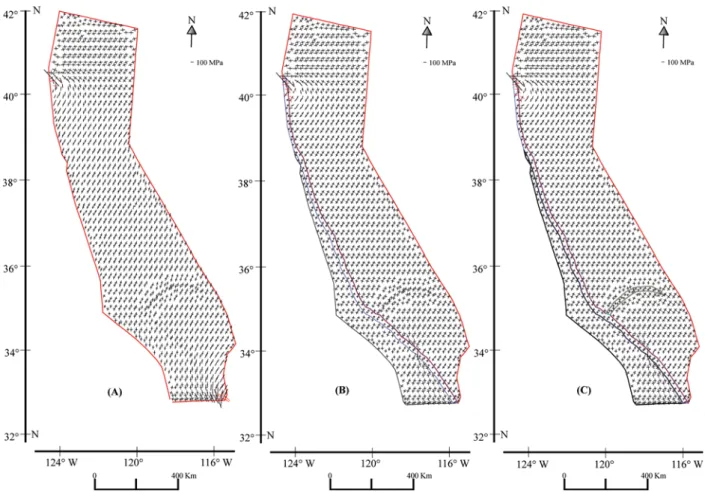
Stress field
The stress field for the three models with increasing displacement is shown in figures 3, 4 and 5. Long lines are the maximum horizontal principal stress σHmaxand
the short lines are the minimum horizontal principal stress σHmin. As the SAFS is in a transpressional regime,
σ1is expected to be equal to σHmax. The red lines in the
models show the tension, while the black lines show the compression. When we consider the one domain model (A), the trend of the maximum horizontal stress is generally NE-SW south of the 40ºN latitude. North of the 40ºN latitude, the trend of the maximum hori-zontal stress is almost E-W. The boundary between both regions is characterized by few NW-SE and NE-SW stress orientations. The southwestern part south of the 35ºN latitude is characterized by a N-S stress ori-entation (Figs. 3A, 4A and 5A). The σHmaxis compres-sive. A similar pattern of the stress field is observed with increasing displacement boundary condition, but the minimum stress (σHmin) with increasing displace-ment boundary condition becomes tensional and the magnitude of σHmax increases. When we consider the three domains model (B) (Figs. 3B, 4B and 5B), the general stress field is similar to that of the one domain model (A), but the magnitude of σHminincreases and it mainly becomes compressive, while again the magni-tude of the σHmin decreases with the increasing
placement boundary condition. South of the latitude of Big Bend near to the SAFS zone, σHmax is more
oblique to the strike of the SAFS but SE of the Garlock Fault some σHmax are perpendicular to the
SAFS strike (Figs. 3B, 4B and 5B). There is no such variation in the stress field in the four domains model (C) with the Garlock Fault. It is similar to the three domains model (B) but the trend of the stress just north of the Garlock Fault is now N-S.
The calculated stress fields in our models are in good agreement with the world stress map (Fig. 6). Both the regional stress field and σHmax orientation in all three models are similar, but models (B) and (C) show a stress perturbation due to SAFS Big Bend and Garlock Fault.
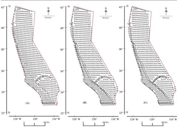
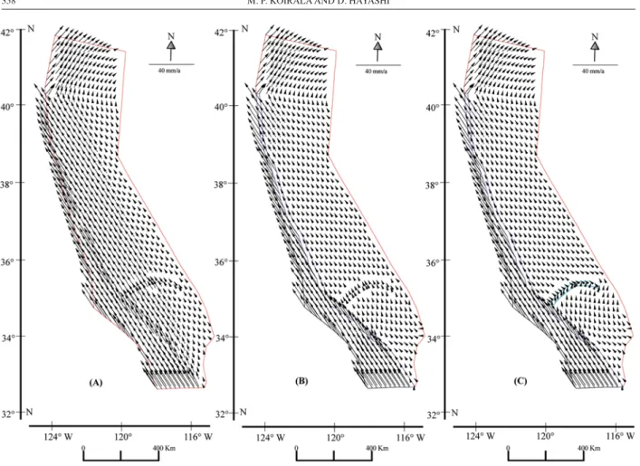
Velocity vector
Velocity vectors for the three models with increasing displacements are shown in figures 7, 8 and 9. In these figures, the arrow shows the direction of motion, while the length of the arrow is the
magni-tude. The general trend of the displacement is towards N34W south of 40ºN latitude, but between 40ºN and 42ºN latitude the displacement is towards N50E direction. Increasing the displacement bound-ary condition causes only an increase in magnitude of the displacement vector (Figs. 7A, 8A and 9A). When we consider the three domains model (Figs. 7B, 8B and 9B), the general trend is the same as in the one domain model (A), but SE of the Big Bend and south of the Garlock Fault the displacement vector is rotat-ed towards north. Increasing displacement boundary condition increases only the magnitude of the dis-placement (Figs. 7B, 8B and 9B). When we consider the four domains model (C), the general trend of the displacement vector is the same as in the three domains model (B) and the magnitude of the dis-placement vector increases with increasing displace-ment. Nevertheless, in the Garlock Fault zone, north of the fault zone the displacement is towards NW and south of the fault zone the displacement is towards NE with high magnitude. Therefore, the Garlock Fault is simulated as a left-lateral strike slip fault in our model. This can be visualized in the models with
increasing displacement boundary condition (Figs. 7C, 8C and 9C).
Our calculated displacement vectors are compara-ble in terms of the regional sense of movement with the velocity model (Flesch et al., 2007) and GPS velocity (Flesch et al., 2007 and references therein), and in our models (B and C) the Big Bend of the SAFS and Garlock Fault have local effects on the displacement vector.
Discussion
Model setup and limitations
Although in nature there are vertical and lateral varia-tions in the rheology, and the material types are inho-mogeneous, the models are constructed considering simplified homogeneous and isotropic domain proper-ties. Elastic rheology is taken for modelling purposes and this is justifiable because 12 km is the seismogenic
depth in the California area. General parameters for the rock domain are based on the published literature as defined above. There are many parallel and subparallel strands of the SAFS but we consider only the biggest and main strand, namely the Garlock Fault. Since the political boundary of the California State is taken as the model area boundary, there may be some boundary effects due to model boundary geometry, but it seems that this effect is very small. As this modelling only considers the elastic thickness of the crust, the effect of the plastic layer below the SAFS and the viscous layer at depth may significantly deviate the results.
Maximum compressive horizontal stress (σHmax)
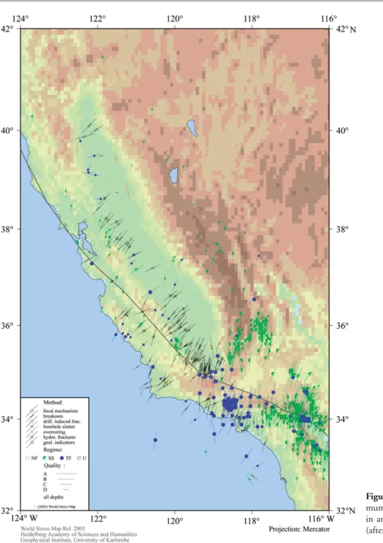
Many methods like borehole breakouts, focal mecha-nisms inversions, drill induced fractures etc., are used for the calculation of the stress fields, especially the max-imum compressive horizontal stress (σHmax). Orientations of the maximum and minimum horizon-tal stresses are calculated by various authors to show the differential stress in the seismogenic depth of California (Parsons, 2006). Most of the measured stresses shown in the world stress map (Fig. 6) and modelled data
(Parsons, 2006) show that the orientation of the maxi-mum horizontal stress is nearly orthogonal to the SAFS along most of its length. The measured maximum prin-cipal stress direction (σHmax) within 20 km from the
fault trace on both sides of the fault shows fault-oblique compression and farther than this distance shows fault-perpendicular compression. In our models, the stress orientations are more or less homogeneously oriented showing fault-oblique compression throughout California and the deviation from this pattern in south-ern California is due to Big Bend and Garlock Fault. Similar results were also obtained by Li and Liu (2006).
Conclusions
The results of this study led us to the following conclu-sions: (1) since the calculated stress field is in good agree-ment with other measured data (borehole breakouts, focal mechanisms inversions and drill-induced fractures) and the calculated displacement vectors are in good agreement with measured GPS velocity, this implies that our imposed boundary condition is able to simulate the present-day tectonic setting. (2) Increasing displacement boundary condition (e.g. Fig. 5A) can produce
al stress σHmin, but σHmax is usually compressive. (3)
Generally, σHmax is oblique to the SAFS. (4) The Big
Bend of the SAFS and Garlock Fault has a local effect on the stress field as well as on the displacement vector which may have significant impact on fault slip, stress, and hence deformation in the surrounding region. Seismicity in southern California may be influenced by the combined effect of the Big Bend and Garlock Fault.
Acknowledgements
M. P. K. is grateful to the Ministry of Education, Culture, Sports, Science, and Technology (Monbukagakusho) of Japan for the scholarship to carry out this research work under the special grad-uate program of the Gradgrad-uate School of Engineering and Science, University of the Ryukyus, Okinawa, Japan.
Figure 8.Velocity vectors at 500 m displacement for models (A), (B), and (C) respectively.
References
ARGUS, D. F. and GORDONR. G. (2001): Present tectonic motion
across the Coast Ranges and the San Andreas fault system in cen-tral California. Geol. Soc. Am. Bull.,113: 1580-1592.
ATWATER, T. (1970): Implications of plate tectonics for the Cenozoic tectonic evolution of western North America. Geol. Soc. Am. Bull.,81: 3513-3635.
BECKEN, M., RITTER, O., PARK, S. K., BEDROSIAN, P. A., WECKMANN, U. and WEBER, M. (2008): A deep crustal fluid channel into the San Andreas Fault system near Parkfield, California. Geophys. J. Int.,173: 718-732. doi: 10.1111/j.1365-246X.2008.03754.x.
BIRDP. and KONGX. (1994): Computer simulations of California tectonics confirm very low strength of major fault. Geol. Soc. Am. Bull.,106: 159-174.
CAI, Y. and WANGC. Y. (2001): Testing fault models with numerical
sim-ulation: example from central California. Tectonophysics,343: 233-238.
CHERYJ., ZOBACKM. D. and HASSANIR. (2001): An integrated mechanical model of the San Andreas fault in central and north-ern California. J. Geophys. Res., 106: 22 051-22 066.
D’ALESSIO, M. A., JOHANSON, I. A., BÜRGMANN, R., SCHMIDT, D.
A. and MURRAY, M. H. (2005): Slicing up the San Francisco Bay
DEMETS, C., GORDON, R. G., ARGUS, D. F. and STEIN, S. (1994): Effects of recent revisions to the geomagnetic reversal time scale on estimates of current plate motions. Geophys. Res. Lett., 21: 2191-2194.
FLESCH, L. M., HOLT, W. E., HAINES, A. J., WEN, L. and SHEN
-TUB. (2007): The dynamics of western North America: stress magnitudes and the relative role of gravitational potential energy, plate interaction at the boundary and basal tractions. Geophys. J. Int., 169: 866-896. doi: 10.1111/j.1365-246X.2007.03274.x.
FUIS, G. S. and MOONEY, W. D. (1990): Lithospheric structure and tectonics from seismic-refraction and other data. In: R. E. WALLACE(ed): The San Andreas Fault System. USGS Professional
Paper, 1515: 207-236.
HAYASHID. (2008): Theoretical basis of FE simulation software
package. Bulletin of Faculty of Science University of the Ryukyus,85: 81-95. http://ir.lib.u-ryukyu.ac.jp/
IRWIN, W. P. (1990): Geology and Plate-Tectonic Development. In: R. E. WALLACE(ed): The San Andreas Fault System. USGS
Professional Paper, 1515: 61-80.
LI, Q. and LIU, M. (2006): Geometrical impact of the San Andreas Fault on Stress and Seismicity in California. Geophys. Res. Lett.,33 (L08302): 1-4. doi: 1029/2005GL025661.
LYNCH, J. C. and RICHARDS, M. A. (2001): Finite elements models of the stress orientations in well-developed strike-slip fault zones: Implications for the distribution for lower crustal strain. J. Geophys. Res., 106: 26 707-26 729.
MALSERVISI, R., GANSC. and FURLONGK. P. (2003): Numerical modeling of strike-slip creeping faults and implications for the Heyward fault, California. Tectonophysics, 361: 121-137.
MINSTER, J. B. and JORDAN, T. H. (1978): Present-day plate
motions. J. Geophys. Res.,83: 5331-6354.
NOSON, L. L., QAMAR, A. and THORSEN, G. W. (1988): Washington State Earthquake Hazards. Washington State Department of Natural Resources, Washington Division of Geology and Earth Resources, Information Circular 85. http://www.pnsn.org/INFO_GENERAL/NQT/welcome.html
PARSONS, T. (2006): Tectonic stressing in California modeled from GPS observations. J. Geophys. Res., 111(B03407): 1-16. doi: 10.1029/2005JB003946.
REINECKER, J., HEIDBACH, O., TINGAY, M., SPERNER, B. and
MÜLLER, B. (2005): The 2005 release of the World Stress Map.
www.world-stress-map.org
SAVAGE, J. C., GAN, W. PRESCOTT, W. H. and SVARCJ. L. (2004): Strain accumulation across the Coast Ranges at the latitude of San
Francisco, 1994-2000. J. Geophys. Res., 109(B03413): 1-11. doi: 10.1029/2003JB002612.
SWANSOND. A., CAMERONK. A., EVARTSR. C., PRINGLEP. T.
and VANCE J. A. (1989): Cenozoic Volcanism in the Cascade Range and Columbia Plateau, Southern Washington, and Northernmost Oregon. AGU Field Trip Guidebook,
T106.http://vulcan.wr.usgs.gov/Volcanoes/PacificNW/AGUT10 6/hood.html#mounthood
WALLACE, R. E. (1990): General Features and Geomorphic Expression. In: R. E. WALLACE (ed): The San Andreas Fault
System. USGS Professional Paper, 1515: 3-21.