Automated hexahedral meshing of knee cartilage structures – application to data from the osteoarthritis initiative

Automated hexahedral meshing of knee cartilage structures - application to data

from the osteoarthritis initiative

B. Rodriguez-Vila , P. Sánchez-González- , I. Oropesa , E. J. Gomez and D. M. Pierce

ABSTRACT

We propose a fully automated methodology for hexahedral meshing of patient-specific structures of the human knee obtained from magnetic resonance images, i.e. femoral/tibial cartilages and menisci. We select eight patients from the Osteoarthritis Initiative and validate our methodology using MATLAB on a laptop computer. We obtain the patient-specific meshes in an average of three minutes, while faithfully representing the geometries with well-shaped elements. We hope to provide a fundamentally different means to test hypotheses on the mechanisms of disease progression by integrating our patient-specific FE meshes with data from individual patients. Download both our meshes and software at

KEYWORDS

Cartilage; meniscus; knee joint; osteoarthritis;

magnetic resonance imaging; finite element analysis; hexahedral mesh

1. Introduction

Articular cartilage in diarthrodial joints must provide (i) a compliant, low-friction surface between the relatively rigid bones; (ii) a long-wearing and resilient surface; and (iii) a means to distribute the contact pressure to the underlying bones. Osteoarthritis (OA) is a disease of the synovial joint, with degeneration and loss of articular car-tilage (and subsequent function) as one hallmark change. OA is a debilitating disease that afflicts nearly 20% of people in the US, costing more than $185.5 billion a year (in 2007 dollars), and its prevalence is projected to increase by about 40% in the next 25 years (Lawrence et al. 2008a, 2008b; Kotlarz et al. 2009).

Fortunately, to facilitate the study of OA we can ac-cess large cohort databases on its progression, e.g. the Osteoarthritis Initiative (OAI) with a cohort of 4,796 participants. The OAI is a multicenter, longitudinal, ob-servational study of knee OA funded in part by the NIH

(Nevitt et al. 2006). This study selects men and women from the general population who are at high risk as in-dicated by weight, knee symptoms, or history of knee injuries. The OAI public database supports investigations of OA of the knee onset and progression using traditional measures of disease and biomarkers. This database in-cludes 3.0 T Siemens Trio Magnetic Resonance Images (MRIs), e.g. localizer (3-plane), intermediate-weighted turbo spin echo, 3-D dual-echo in steady-state (DESS),

intermediate-weighted turbo spin echo, Tl-weighted 3-D flash, and T2.

Despite the multifactorial nature of OA, mechanical stresses play a key role in the destructive evolution of the disease (Andriacchi et al. 2004; Goldring and Marcu 2009; Polur et al. 2010; Loeser et al. 2012) and subsequent loss of tissue/joint function. Both overloading (e.g. trauma) and reduced loading (e.g. immobilization) of cartilage induce molecular and microstructural changes that lead to me-chanical softening, fibrillation, and erosion. Experiments can be used to quantify mechanical properties and biol-ogy of tissues, and imaging can be used to estimate tissue structure and even strains; however, only computational models can estimate intra-tissue stresses in human joints, because the required in vivo experiments are impossible or unsafe. Finite element (FE) models are well-established at the macro (e.g. joint) scale as a means to estimate intra-tissue stress distributions.

arbitrary geometries, cf. Yerry and Shephard (1984), Lohner and Parikh (1988).

Building computational meshes from hexahedra is far more restrictive and time consuming, and a fully auto-matic algorithm for generating hexahedral meshes of ar-bitrary geometries does not yet exist. However, for a wide range of applications, hexahedral-based meshes are pre-ferred. Among many reasons, FE meshes require far more tetrahedral elements (relative to hexahedral elements) to achieve the same solution accuracy for a given analyses, and this leads to higher computational costs (both time and memory) (Ramos and Sim5es 2006). When the aim is to apply FE analyses, tetrahedral meshes produce accept-able displacement results but are relatively inaccurate for predicting stresses (Puso and Solberg 2006). Addition-ally, we aim to allow use of different material parameters through the thickness of the tissue to model the zonal structure of healthy cartilage (Pierce et al. 2013a, 2013b).

In this case hexahedral meshes are an excellent option.

Specialized software packages, such as TrueGrid (XYZ Scientific Applications, Inc., Pleasant Hill, CA), MeshGems (Distene SAS, Bruyeres-le-Chatel, FR) and IA-FEMesh (Grosland et al. 2009), simplify the creation of fully hexahedral meshes. Nonetheless, such software demands significant experience and user interaction to create a block layout for each structure from which meshes are then generated. Each structure may thus re-quire significant processing time, on the order of several hours per structure.

Several methods for generic hexahedral meshing are proposed in the literature, e.g. octree-based (Maréchal

2009), morphing-based (Murase and Tamamura 2016),

and sweeping (Roca et al. 2004; Lievers and Kent 2013; Mukherjee et al. 2013). Of these only the method of

Murase and Tamamura (2016) was tested on structures in the knee, and unfortunately little information on results is available.

'Open Knee(s): Virtual Biomechanical Represent-ations of the Knee Joint' (Erdemir 2016) offers patient-specific biomechanical models of knee structures based on hexahedral meshes. The project provides specific meshes, generated using TrueGrid, for download but does not provide software to generate new models based on additional patient images.

In this work we propose a specific, automatic algo-rithm designed to work with patient-specific geometries of the knee obtained from MRI. Indeed, we establish a fully automated methodology for hexahedral meshing of knee joint structures, i.e. femoral cartilage, menisci, and tibial plateau cartilages.

2. Materials and methods

2.7. Segment and reconstruct image data

We determine the anatomical structures of the knee in each patient by manually segmenting sagittal slices of the fat-suppressed 3-D dual-echo in steady state (DESS), e.g. from the OAI database. MRI data sets from the OAI include 160 slices of 384 x 384 pixels2, for a final voxel res-olution of 0.365 x 0.365 x 0.7 mm3. The DESS sequence provides excellent universal cartilage discrimination to capture quantitative cartilage morphology. We gener-ate triangular surface meshes of each structure from the manual segmentations using a marching cubes algorithm

(Lorensen and Cline 1987), see Figure 1.

2.2. Generate hexahedral meshes

We start from triangular surfaces of the structures of in-terest as inputs to our fully-automatic, hexahedral mesh-ing methodology for knee joint structures, specifically femoral cartilage, medial/lateral menisci, and medial/ lateral tibial cartilages.

2.2.7. Overview

Our methodology uses the following steps for each struc-ture of interest: (1) create an initial low-resolution mesh with our structure-specific, custom sweeping algorithm, (2) smooth this mesh using a Laplacian filter, (3) ex-pand this mesh to fit the original (triangular surface) segmentation, (4) optimize element quality, (5) refine this by subdividing hexahedra, and (6) smooth, expand and optimize element quality iteratively. The first five steps of our methodology follow Lievers and Kent (2013) while we perform step (6) iteratively until all the elements of the mesh fulfill the quality conditions.

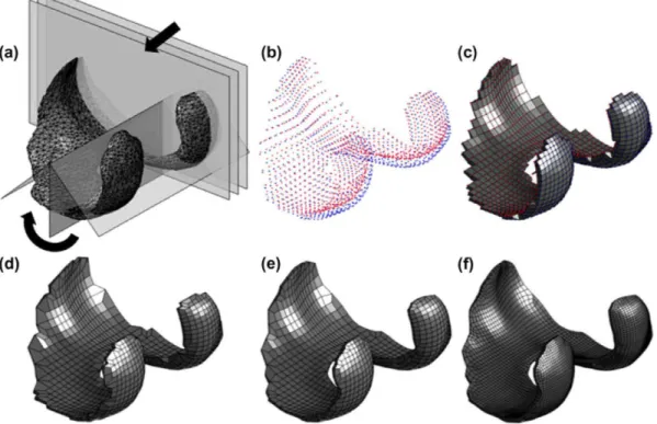
Femoral cartilage: First we outline our custom hexa-hedral meshing methodology for femoral cartilage struc-tures, see Figure 2.

Figure 1. We manually segment magnetic resonance ¡mages and generate triangular surfaces using a marching cubes algorithm, (a) representative fat-suppressed 3-D dual-echo in steady state (DESS) images with manual segmentation, and (b) resulting triangular surfaces of each patient-specific structure.

(b)

„,

Figure 2. Schematic representation of custom hexahedral mesh generation for femoral cartilage structures: (a) sweeping in both axial

and circumferential directions using cylindrical coordinates, (b) determining initial nodes, (c) generating initial low-resolution mesh, (d) correcting elements with six nodes (collapsed elements), (e) smoothing the mesh, and (f) refining and optimizing the mesh iteratively.

as nodes of an initial non-smooth mesh (Figure 2(c)). We detect and process elements formed by only six nodes (collapsed elements) (Figure 2(d)) before applying Lapla-cian smoothing (Field 1988) (Figure 2(e)). Once we have this initial hexahedral mesh, we refine it and iteratively smooth, expand and optimize the mesh, until all of the elements of the final mesh fulfill the minimum quality metrics (Figure 2(f)).

Menisci: Next we outline our custom hexahedral meshing methodology for meniscus structures in Figure 3.

We model each meniscus using a radial sweeping al-gorithm with the proximal-distal (vertical) line through the center of mass of each respective tibial cartilage as

principal axis (Figure 3(a)). We initially describe each 2-D contour as a triangle to posteriorly define ten patches and 17 points (Figure 3(b)). We use the resulting cloud of points (Figure 3(c)) to create the initial low-resolution mesh, and apply Laplacian smoothing to eliminate out-liers (Figure 3(d)). Thereafter we refine this mesh and iteratively smooth, expand and optimize it, until all of the elements of the final mesh fulfill the minimum quality metrics (Figure 3(e)).

Tibial plateau cartilages: Finally, we outline our cus-tom hexahedral meshing methodology for tibial cartilage structures in Figure 4.

dis-I i f J ;-.,

*3B

Figure 3. Schematic representation of custom hexahedral mesh generation for meniscus structures: (a) sweeping in the circumferential

direction using cylindrical coordinates, (b) modeling each contour as a triangle with ten patches and 17 nodes, (c) determining initial nodes, (d) generating initial low-resolution mesh, and (e) refining and optimizing the mesh iteratively.

kill/

'"•'•• X'vSV• V •."•-•.:•*:?•>* ••

•••is ••-• ¡>*V».• ;--Vr,*'-" •*'• * •*

*»«L,. i'V/-,* i.'¥ j« ' - »t: - * . \v ;**v-^*+\+ •utSKiíV .'^Vj- • "--vA1"-"/*™*"''

'*'. J M B " ; .-••. * - ,:V'V.ll, ••»:•

•'.•-/ i i ¡ T I

Figure 4. Schematic representation of custom hexahedral mesh generation for tibial cartilage structures: (a) first sweeping in Cartesian

coordinates, (b) second sweeping in Cartesian coordinates, (c) determining initial nodes, (d) generating initial low-resolution mesh, and (e) refining and optimizing the mesh iteratively.

tribution, centered at the center of mass of the structure (Figure 4(a)), with a radial distribution (Figure 4(b)). We compute the intersection of rays with the triangular surfaces. As in the first case, the result is two clouds of points describing the proximal (articular surface, red) and distal (blue) surfaces of the cartilage (Figure 4(c)). We use these points as nodes of an initial non-smooth hexahedral mesh (Figure 4(d)). Once we have this initial mesh, we refine it and iteratively smooth, expand and

optimize the mesh, until all of the elements of the final mesh fulfill the minimum quality metrics (Figure 4(e)).

2.2.2. Create low-resolution meshes

Our methodology uses the minimum bounding box

meshes, while eliminating the use of collapsed elements. Creation of the initial low-resolution mesh is the main difference between our structure-specific methods, while the processes of smoothing, expanding and optimization of the meshes are common between structures.

2.2.3. Smooth meshes with Laplacian filter

We first perform Laplacian smoothing over all nodes of the low-resolution mesh, an enhancement process that removes outliers (Field 1988). For each vertex formed at nodal position n¡ in our mesh (z e {1,2,... ,N} with N nodes in the mesh), we select a new nodal position ñ¡ based on local information using an extended version of the Laplacian smoothing algorithm (Vollmer et al. 1999)

as

1

ñ; = an; -\ > n, (1) ||adj(i)|| ^eadjCO }

where ny are the positions of nodes forming adjacent vertices j e adj(z') (if adj(z') = 0 then node z is not moved). We use a = 0.5 to balance smoothing quality and degree of model shrinkage.

2.2.4. Expand meshes into the triangular surfaces

Laplacian smoothing reduces the volume of our struc-tures, and thus we assume our deformation step is only for expansion. We expand meshes using only the surface nodes. In the femoral and tibial cartilages, the struc-tures have only surface nodes before division into layers. However, in the menisci there are internal nodes. In this case, we move (if needed) internal nodes during the optimization step.

We deform each surface node n¡ towards its respective triangular surface along a vector v¡ determined from the average of all the face normals sharing n,-. We compute each face normal as the unit vector resulting from the cross product of both edges sharing n¡ and the face of interest. The intersection of the ray, with origin n¡ and direction v¡, and the triangular surface mesh determines the new position ñ¡. If we do not find an intersection, or the intersection is very far from the origin, n¡ is not modified.

2.2.5. Optimize meshes

Creation or expansion of the low-resolution mesh may result in mesh distortion or inversion. Thus, we perform an optimization step to both repair any invalid elements and improve the overall mesh quality. To achieve these goals, we propose combining Laplacian smoothing and element optimization, an approach that works indepen-dent of the resolution of the mesh. First, we detect ele-ment inversions as negative nodal Jacobian fa values, cf. (2) in Section 2.3. We solve this problem by replacing such nodes with the average of its neighbors. Second,

Figure 5. Schematic representation of mesh optimization. We

move nodes associated with angles <45° or >135° (white dots) to new positions (white squares) in order to improve the scaled Jacobian values and meet minimum quality metrics.

we apply local mesh improvements to ill-conditioned elements with scaled Jacobians / < 0.5, cf. (3), following a strategy similar to that proposed by Auer and Gasser (2010). For each ill-conditioned element, we detect and correct internal angles <45° or >135°. To illustrate, in Figure 5 we move nodes 1 and 3 (associated with obtuse angles >135°) further apart from one another along the line connecting them, while we move nodes 2 and 4 (associated with acute angles <45°) closer together to one another along the line connecting them.

2.2.6. Refine meshes

For the femoral and tibial cartilages, where the initial low-resolution mesh is only one-element thick, we divide each hexahedral element into four hexahedra (dividing by two in the lateral-medial and anterior-posterior directions, but not in the proximal-distal direction). For the menisci, we divide each hexahedral element into eight hexahedra (dividing by two in each of the three sweeping directions). Importantly, by modifying the sweeping parameters we can fully adjust the density of our meshes.

2.2.7. Smooth, expand and optimize iteratively

The first five steps of our methodology, outlined in Section 2.2.1, follow Lievers and Kent (2013) while we perform step (6) iteratively until all the elements of the mesh fulfill the quality conditions. Our iterative approach allows us to meet or exceed minimum targets for our quality metrics outlined in Section 2.3,

Table Al in Appendix 1 provides pseudo code for our structure-specific cartilage meshing methodology.

2.3. Determine quality of the meshes

is a common quality metric (De Santis et al. 2011). We evaluate the nodal Jacobian/^ of each hexahedral element at the element center k = 0 using the principal axes, and at each node k, k e [ 1 , . . . , 8], as the triple scalar product of the edges connected to that node using

Jk = eui • (eui x eui)- (2)

The modulus of (2) represents six times the volume of the tetrahedron enclosed by these three edges. We evalu-ate the scaled Jacobian / of an element as the minimum of each nodal Jacobian fa divided by the length of the three corresponding edges (eui, efc2> «tó) using

/ = min fcs[0,...,8]

Jk |e*illl|e*2lll|efc»l

(3)

where / e [—1,1] for a hexahedral element, with —1 corresponding to the worst possible elements and +1 the best possible ones. Importantly, only elements with a non-zero, positive scaled Jacobian are suitable for FE analyses. We use the open-source program ParaView (Kitware, Inc., Clifton Park, New York, USA) to evaluate the scaled Jacobian, among other quality metrics, which in turn uses the Verdict library (Stimpson et al. 2007; Ayachit2015).

We evaluate the similarity of our hexahedral meshes to the original triangular surfaces using the non-signed value of the Hausdorff distance (Aspert et al. 2002). We compute the error e^ for each node m^ in the original triangular surface (k e {1,2,... ,M} with M nodes in the mesh) as the infimum of the distance between m^ and all nodes n¡ in our custom hexahedral mesh (z e {1,2,... ,N} with N nodes in the mesh)

e/c inf di;

>e{i,2,...,N} ' (4)

where c//y is the Cartesian distance from m^ to n¡ (NB. this distance is not symmetric). We use the open-source program 3D Sheer (http://www.slicer.org) to evaluate the error in distance for each node (Fedorov et al. 2012).

2.4. Validate methodology

To validate the efficacy of our methodology, and to eval-uate its performance, we implemented it in MATLAB 2016a (The MathWorks Inc., Natick, MA). We select eight patients from the OAI database, manually segment the cartilages and menisci using the DESS images, and generate triangular surface meshes of each structure, cf Section 2.1. Finally, using eight triangular surface meshes, we test our methodology using a laptop computer with an Intel Core Í7-3632QM CPU at 2.20 GHz and with

8 GB RAM. For each of the eight tests we record the total number of elements, the quality (scaled Jacobian) of each element, the root-mean-squared error (RMSE, between the surface and hexahedral meshes), and computation time.

In our example meshes we adjust the mesh density, i.e. we select parameters controlling the spatial resolution, so that the mean value of the edge lengths of the elements is ~ 1 mm for all of the structures. For the femoral and tibial cartilages we chose to create distinct layers to mimic the superficial/middle/deep zones of cartilage (each with two elements per layer) using anatomically correct through-thickness ratios (0.16/0.54/0.30) (Mow and Huiskes 2005; Fujioka et al. 2013). In this way we allow use of differ-ent material parameters to model the zonal structure of healthy cartilage, cf. Pierce et al. (2013a, 2013b).

2.5. Analyze outputs

First we check if our results are normally distributed using a Shapiro-Wilk test with a significance level of 0.05 (Royston 1992). If number of elements, number of elements binned by quality (/ > 0.8 or 0.6 > / > 0.5), RMSE distance, computation time, and supplementary element data (on resolution) are normally distributed, we report the mean and standard deviation (M±SD), otherwise we report the median and interquartile range (MD[Q1,Q3]).

3. Results

Using our fully automated methodology, we generate hexahedral meshes of patient-specific geometric struc-tures of the human knee - i.e. femoral cartilages, menisci, and tibial cartilages - for eight patients from the OAI database. Figure 6 illustrates two representative meshes generated using our methodology.

With our methodology, cartilages can be meshed with any number of elements through their thickness. This flexibility allows us to represent cartilage using a single constitutive model, as in Figure 6(a) (where we represent the full cartilage thickness with a single color), or as a three-layered material with different constitutive models, as in Figure 6(b) (where we represent the three different layers with different colors).

3.1. Results by anatomical structure

Figure 6. Representative hexahedral meshes of the femoral (yellow) and tibial (blue) cartilages, and medial (red) and lateral (green) menisci where the structures are separated in the axial direction for visualization purposes: (a) healthy structures of patient 9932809, and (b) degenerated structures of patient 9951449.

14

12

JS

§ io

i

S 8 "S

I!

9 4

2

x l ( ) - '

| medial meniscus | Lotero] meniscus I medial tibia

J lateral tibia femur

— . „ . .

.

„

..n .11

Scaled Jacobian

(a) ()..->

0.6 0.7 0.8 Scaled Jacobian

>0.9

Figure 7. The quality of eight patient-specific meshes measured using the scaled Jacobian, (a) histogram of the resulting scaled Jacobian

values, and (b) representative spatial distribution of the scaled Jacobian from patient 9948792 (expanded in the axial direction for visualization).

of elements binned by quality (/ > 0.8 or 0.6 > / > 0.5), and RMSE distances are normally distributed, and we present these results using the mean and standard deviation (M±SD). In contrast, computation time cannot be modeled as a normal distribution and thus we present these results using the median and interquartile range (MD[Q1,Q3]).

Table 1 provides the mesh quality metrics by anatom-ical structure, and corresponding computation times.

Importantly, every structure-specific mesh comprises only hexahedral elements - no collapsed elements or wedges are necessary - and with all scaled Jacobian values / > 0.5. Furthermore, both femoral and tibial cartilages comprise ~95% of their elements with / > 0.8 on average, and less than 0.5% of their elements with 0.6 > / > 0.5. Both of these structures present excellent similarity in shape and size to their original surface meshes, RMSE distances below 0.2 mm.

In contrast, our methodology obtains poorer perfor-mance for the menisci, both in time, mesh quality and

error. Although menisci represent only ~ 10% of the ele-ments required to model a patient, they require approxi-mately two-thirds of the processing time.

Figure 7 illustrates the overall mesh quality from our validation study on eight patient-specific meshes of the structures of interest. Specifically, Figure 8(a) illustrates the quality of eight patient-specific meshes using a his-togram of the scaled Jacobian values of the five structures. The number of high-quality elements in the femoral and tibial cartilages masks the results in the menisci, where a more homogeneous distribution is observed. All the elements have scaled Jacobian values >0.5, and ~90% of them are high-quality elements. Figure 7(b) illustrates a representative spatial distribution of the scaled Jacobian from patient 9948792. Most of the lower-quality elements are in the menisci, the edges of the femoral cartilage, and the transitions from Cartesian to angular sweeping in the tibial cartilages.

x l();

4

3

2

1

| moclial meniscus | lateral meniscus | medial tibia

| lateral tibia

Zi femur •

•

_ _ J ] O ^_o ,

Distance Error (nun)

0.5 1.0 1.5 2.0 >2.0 (a) Distante Errar (mm)

Figure 8. The quality of eight patient-specific meshes measured using the Haussdorff distance between the input triangular surfaces and resulting hexahedral meshes, (a) histogram of the resulting distance errors, (b) representative spatial distribution of the distance errors from patient 9988820 (RMSE = 0.2 mm).

Table 1. Mesh quality metrics by anatomical structure (M±SD), where F. = Femoral, T. = Tibial, L. = Lateral, and M. = Medial, and corresponding computation time (MD[Q1,Q3]). RMSE = Root-Mean-Squared-Error in Hausdorff distance between the input triangular surfaces and resulting hexahedral meshes.

Structure

F. Cartilage L. Meniscus M. Meniscus L.T. Cartilage M.T. Cartilage

Elements (#)

18713 ±1875 1675 ± 2 0 6 1380 ± 2 0 0 3816 ± 0 3906 ± 0

J > 0.8 (%)

95.66 ± 0.89 62.07 ±7.53 56.84 ± 8.83 93.76 ± 3 . 5 8 95.78 ± 1 . 4 6

0.6 > J > 0.5 (%)

0.48 ± 0 . 1 6 3.05 ± 2 . 1 0 5.28 ± 2 . 2 6 0.17 ± 0 . 3 0.05 ±0.11

RMSE (mm)

0.242 ± 0.024 0.334 ± 0.082 0.543 ±0.173 0.139 ±0.019 0.128 ±0.027

Time(s)

30.0 ±[29.8,31.3] 60.5 ±[45.3,73.0] 43.5 ±[31.0,66.8] 5.7 ±[5.5,6.0] 6.2 ±[5.7,6.4]

the structures of interest. Specifically, Figure 8(a) illus-trates the quality of eight patient-specific meshes using a histogram of the Haussdorff distance between the initial triangular surfaces and resulting hexahedral meshes of the five structures. We see that almost all of the distance errors in all the structures are below 0.5 mm. Higher values are in the edges of the structures, particularly in the femoral cartilage and the extremes of the menisci. Figure 8(b) illustrates a representative spatial distribution of the distance errors from patient 9988820.

Table Bl in Appendix 2 provides mean and minimum values of edge length, face area and element volume by structure. All variables are normally distributed.

structures of the human knee obtained from MRIs, and demonstrate its performance. Our methodology allows modeling of both normal/healthy knee structures (i.e. those without clear signs of degeneration), as shown in Figure 6(a), and pathological knee structures (i.e. those presenting signs of degeneration), as shown in Figure 6(b) where both the femoral and medial tibial cartilages present holes in their anatomy. However, such holes (complete local loss of tissue) in the structures can only be modeled if they are detected in the initial low-resolution mesh. We could use a higher sweeping resolution in our initial mesh to lower the distance errors at the expense of a higher mesh density and increased computation time.

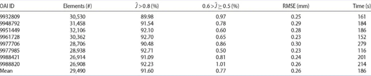
3.2. Results by OAI patient

Table 2 provides the mesh quality metrics by OAI patient ID, and corresponding computation times. The method-ology gives consistent performance across all patients selected, except in terms of computation time. Meshes from patient 9977985 took less than two minutes to gen-erate, while meshes from patient 9977706 took more than four and a half minutes. The remaining patients present computation times of approximately three minutes.

4. Discussion

In this work, we propose a novel methodology for gener-ating high-quality, hexahedral meshes of patient-specific

4.1. Relation to state-of-the-art

Table 2. Mesh quality metrics by OAI patient ID, where RMSE = triangular surfaces and resulting hexahedral meshes.

OAI ID Elements (#) j>0.8(%)

9932809 30,530 89.98 9948792 31,458 91.54 9951449 32,106 92.10 9961728 30,362 92.70 9977706 28,706 90.48 9977985 28,938 92.71 9988421 26,914 91.09 9988820 26,908 92.23 Mean 29,490 91.60

Within the context of the FE method, the quality of the finite elements obtained from mesh generation greatly affects both the convergence of the simulations and the resulting approximations to the solutions of the govern-ing partial differential equations. Additionally, accuracy in the representation of the true, patient-specific in vivo geometry also influences the biomechanical/biomedical applicability of the results. Metrics for mesh quality must detect inverted elements (elements with negative volume, which generate meaningless results or prevent solution convergence) and provide an estimate of the mesh's fit-ness for use in numerical simulations.

Only IA-FEMESH published an evaluation of mesh accuracy and validity (DeVries et al. 2009), but this study focused specifically on phalanx bones. The authors re-ported computational times of approximately six minutes for one mesh of 4550 elements, where 10% of the elements were distorted. Our methodology generates meshes of five patient-specific structures in approximately three minutes (on average) with ~30,000 elements in total, and where less than 1% are acceptable but not high-quality elements.

The NIH-sponsored project 'Open Knee(s): Virtual Biomechanical Representations of the Knee Joint' offers free access to hexahedral meshes of almost ten specific patients. Similarly, we offer free access to our meshes of eight patients from the OAI database (formatted for multiply FE codes). Additionally, we offer our MATLAB implementation of our methodology free for download. Thus, interested researchers can generate specific meshes well suited to FE simulation based only on their segmen-tations of MRIs.

4.2. Summary and future work

Our fully hexahedral meshing methodology preserves tissue volume and produces high-quality elements. To the best of our knowledge, no other automatic hexahedral meshing for patient-specific knee structures exists in the literature. With our freely available MATLAB implemen-tation, there are low barriers to use since users need only

Root-Mean-Squared-Error in Hausdorff distance between the input

0.6>j>0.5(%) RMSE (mm) Time(s)

0.97 0.25 161 0.78 0.29 184 0.60 0.28 186 0.65 0.23 152 0.86 0.30 279 0.50 0.23 116 0.81 0.24 201 1.01 0.26 214 0.77 0.26 186

input triangular surface segmentations and choose the initial resolution for the mesh of each structure. Down-load both our meshes and software at http://im.engr.

uconn.edu/downloads.php.

We hope to provide a fundamentally different means to test hypotheses on the mechanisms of disease pro-gression at the patient level by integrating our patient-specific FE meshes and analysis framework, cf. Pierce et al. (2016), with data from individual patients or from natural history databases, e.g. the OAI. In the longer term, simulation-based, predictive medicine combined with medical imaging will likely improve the health, well-being, and quality of life for patients with O A.

Acknowledgements

We thank Phoebe Szarek for searching the OAI database and selecting patients for our validation study.

Disclosure statement

No potential conflict of interest was reported by the authors.

Funding

This work was supported by the Mobility Grants from Networking Research on Bioengineering, Biomaterials and Nanomedicine (BRV) and the National Science Foundation [CAREER 1653358] (DMP).

References

Andriacchi TP, Mündermann A, Smith RL, Alexander EJ, Dyrby CO, Koo S. 2004. A framework for the in vivo pathomechanics of osteoarthritis at the knee. Ann Biomed Eng. 32:447-457.

Aspert N, Santa-Cruz D, Ebrahimi T. 2002. Mesh: measuring errors between surfaces using the hausdorff distance. Proceedings of the IEEE International Conference in Multimedia and Expo (ICME). Lausanne, Switzerland; p. 705-708.

Ayachit U. 2015. The paraview guide: a parallel visualization application. Clifton Park (NY): Kitware Inc.

De Santis G, De Beule M, Van Canneyt K, Segers P, Verdonck P, Verhegghe B. 2011. Full-hexahedral structured meshing for image-based computational vascular modeling. Med Eng Phys. 33:1318-1325.

DeVries NA, Shivanna KH, Tadepalli SC, Magnotta VA,

Grosland NM. 2009. IA-FEMESH: anatomic fe models - a

check of mesh accuracy and validity. Iowa Orthop J. 29:48-54.

Erdemir A. 2016. Open knee: open source modeling &

simulation to enable scientific discovery and clinical care in knee biomechanics. J Knee Surg. 29:107-16.

Fedorov A, Beichel R, Kalpathy-Cramer J, Finet J, Fillion-Robin JC, Pujol S, Bauer C, Jennings D, Fennessy F, Sonka M, et al. 2012. 3D slicer as an image computing platform for the quantitative imaging network. Magn Reson Imaging. 30:1323-41.

Field DA. 1988. Laplacian smoothing and delaunay

triangulations. Commun Appl Numer Meth. 4:709-712. Fujioka R, Aoyama T, Takakuwa T. 2013. The layered structure

of the articular surface. Osteoarthritis Cartilage. 21:1092-1098.

Goldring MB, Marcu KB. 2009. Cartilage homeostasis in health and rheumatic diseases. Arthritis Res Ther. 11:224.

Grosland NM, Bafna R, Magnotta VA. 2009. Automated

hexahedral meshing of anatomic structures using deformable registration. Comput Methods Biomech Biomed Eng. 12:35-43.

Kotlarz H, Gunnarsson CL, Fang H, Rizzo JA. 2009. Insurer and out-of-pocket costs of osteoarthritis in the us: evidence from national survey data. Arthritis Rheum. 60:3546-3553. Lawrence RC, Felson DT, Helmick CG, Arnold LM, Choi H,

Deyo RA, Gabriel S, Hirsch R, Hochberg MC, Hunder GG, et al. 2008a. Estimates of the prevalence of arthritis and other rheumatic conditions in the united states: Part ii. Arthritis Rheum. 58:26-35.

Lawrence RC, Felson DT, Helmick CG, Arnold LM, Choi H, Deyo RA, Hirsch SGR, Hochberg MC, Hunder GG, Jordan JM, et al. 2008b. National arthritis data workgroup, estimates of the prevalence of arthritis and other rheumatic conditions in the united states: Part ii. Arthritis Rheum. 58:26-35. Lievers WB, Kent RW. 2013. Patient-specific modelling of the

foot: automated hexahedral meshing of the bones. Comput Methods Biomech Biomed Eng. 16:1287-1297.

Loeser RF, Goldring SR, Scanzello CR, Goldring MB. 2012.

Osteoarthritis: a disease of the joint as an organ. Arthritis Rheum. 64:1697-1707.

Lohner R, Parikh P. 1988. Generation of three-dimensional unstructured grids by the advancing-front method. Int J Numer Meth Fluids. 8:1135-1149.

Lorensen WE, Cline HE. 1987. Marching cubes: a high

resolution 3D surface construction algorithm. Comput Graph. 21:163-169.

Maréchal L. 2009. Advances in octree-based all-hexahedral mesh generation: handling sharp features. In: Clark BW, editors. Proceedings of the 18th International Meshing Roundtable. Berlin, Heidelberg: Springer, p. 65-84.

Mow VC, Huiskes R. 2005. Structure and function of ligaments and tendons. In: Woo SLY, Lee TQ, Abramowitch SD, Gilbert TW, editors. Basic orthopaedic biomechanics and mechano-biology. Philadelphia (PA): Lippincott Williams & Wilkins. p. 301-342.

Mukherjee N, Peddi B, Cabello J, Hancock M. 2013. Automatic hexahedral sweep mesh generation of open volumes. In: Jiao X, Weill JC, editors. Proceedings of the 21st International Meshing Roundtable. Berlin, Heidelberg: Springer, p. 333-347.

Murase K, Tamamura S. 2016. Hexahedral meshing techinique with high fidelities and accuracies for knee FEA. Bone Joint J. 98-B:60.

Nevitt MC, Felson DT, Lester G. 2006. The osteoarthritis initiative: protocol for the cohort study. San Francisco: The Osteoarthritis Initiative, University of California. http://oai.

epi-ucsf.org/datarelease/docs/StudyDesignProtocol.pdf.

O'Rourke J. 1985. Finding minimal enclosing boxes. Int J Comput Inform Sci. 14:183-199.

Pierce DM, Ricken T, Holzapfel GA. 2013a. A hyperelastic biphasic fiber-reinforced model of articular cartilage con-sidering distributed collagen fiber orientations: continuum basis, computational aspects and applications. Comput Methods Biomech Biomed Eng. 16:1344-1361.

Pierce DM, Ricken T, Holzapfel GA. 2013b. Modeling

sample/patient-specific structural and diffusional response of cartilage using DT-MRI. Int J Numer Meth Biomed Eng. 29:807-821.

Pierce DM, Unterberger MJ, Trobin W, Ricken T, Holzapfel GA. 2016. A microstructurally based continuum model of cartilage viscoelasticity and permeability incorporating statistical fiber orientation. Biomech Model Mechanobiol. 15:229-244.

Polur I, Lee PL, Serváis JM, Xu L, Li Y. 2010. Role of HTRA1, a serine protease, in the progression of articular cartilage degeneration. Histol Histopathol. 25:599-608.

Puso MA, Solberg J. 2006. A stabilized nodally integrated tetrahedral. Int J Numer Meth Biomed Eng. 67:841-867. Ramos A, Simoes J A. 2006. Tetrahedral versus hexahedral finite

elements in numerical modelling of the proximal femur. Med Eng Phys. 28:916-924.

Roca X, Sarrate J, Huerta A. 2004. Surface mesh

projection for hexahedral mesh generation by sweeping. In: Üngór A, editors. Proceedings of the 13th Interna-tional Meshing Roundtable. Berlin, Heidelberg: Springer, p. 169-180.

Royston P. 1992. Approximating the Shapiro-Wilk w-test for non-normality. Stat Comput. 2:117-119.

Stimpson CJ, Ernst CD, Knupp PM, Pebay PP, Thompson DC.

2007. The verdict geometric quality library. Albuquerque, NM and Livermore, CA; Sandia National Laboratories, SAND2007-1751.

Vollmer J, Mencl R, Müller H. 1999. Improved Laplacian

smoothing of noisy surface meshes. Comput Graph Forum. 18:131-138.

Appendix 1. Pseudo code for the meshing methodology

Table A1. Pseudo code for our structure-specific cartilage meshing methodology.

for pre-processing do

Compute minimal bounding box for femoral and tibial cartilages Compute center-of-mass for both tibial plateau cartilages Compute two points defining the axis for the femoral cartilage

end for

for femoral cartilage do

cylindrical sweep process six-node elements Laplacian smooth expand to triangular surface optimize

refine

while scaled Jacobian < 0.5 do

Laplacian smooth expand to triangular surface optimize

end while

divide into through-thickness layers

end for

for each meniscus do

radial sweep parameterize contour Laplacian smooth expand to triangular surface optimize

refine

while scaled Jacobian < 0.5 do

Laplacian smooth expand to triangular surface optimize

end while end for

for each tibial plateau cartilage do

Cartesian sweep radial sweep

while scaled Jacobian < 0.5 do

Laplacian smooth expand to triangular surface optimize

end while

divide into through-thickness layers

end for

Appendix 2. Supplementary data on elements in the example meshes

Table B1. Supplementary data on elements in the example meshes organized by anatomical structure (M±SD), where F. = Femoral, T. = Tibial, L. = Lateral, M. = Medial, E.L. = edge length (mm), F.A. = face area (mm2), and E.V. = element volume (mm3).

Structure mean(E.L.) min(E.L.) mean(FA) min(F.A.) mean(E.V.) min(E.V.)