Tracking moving optima using Kalman-based predictions

Claudio Rossi

Universidad Polit´ecnica de Madrid, Madrid, 28006, Spain

Mohamed Abderrahim

Departamento de Ingenier´ıa de Sistemas y Automatica,

Universidad Carlos III de Madrid, Legan´es (Madrid), 28911, Spain

Julio C´esar D´ıaz

Departamento de Ingenier´ıa de Sistemas y Automatica,

Universidad Carlos III de Madrid, Legan´es (Madrid), 28911, Spain

Abstract

The dynamic optimization problem concerns finding an optimum in a changing en-vironment. In the field of evolutionary algorithms, this implies dealing with a time-changing fitness landscape. In this paper we compare different techniques for integrat-ing motion information into an evolutionary algorithm, in the case it has to follow a time-changing optimum, under the assumption that the changes follow a nonrandom law. Such a law can be estimated in order to improve the optimum tracking capa-bilities of the algorithm. In particular, we will focus on first order dynamical laws to track moving objects. A vision-based tracking robotic application is used as testbed for experimental comparison.

Keywords

Evolutionary algorithms, vision-based tracking, dynamic optimization problem, time-varying fitness function.

1

Introduction

Real-world applications often deal with a highly noisy and changing environment. Evolutionary algorithms (EAs) are known to be well suited for dealing with noisy input information, and can cope with a changing environment, since the search is performed by constantly (at each new generation) producing new candidate solutions. Thus, they inherently consider time: newly generated individuals can be subject to time-changing constraints and/or evaluated and selected according to a time-varying fitness function. Furthermore, under certain circumstances, since individuals tend to be scattered around the optimum, there is a good probability that when the optimum moves, one of the individuals of the population will be close enough to still represent a good solution of the problem under study.

suitable degree of population diversity, in order to guarantee an adequate level of explo-ration and to avoid the algorithm to concentrate on the current optimum. An excessive convergence would make the algorithm miss important changes in the environment, while a spread out population can adapt to changes more easily. The literature on dy-namic optimization problems has focused on dealing with the changing environment by means of

1. Dynamic parameters control (Angeline, 1997; B¨ack, 1998), and specialized adaptive operators (Cobb, 1990), also making use of local search techniques (Vavak et al., 1996) or information theoretic based methods (Abbass et al., 2004). The latter tries to get an insight into the problem of identifying relevant substructures and ex-ploits the substructures to respond to changes in the environment. The cumulative step length adaptation mechanism is used in Arnold and Beyer (2006) to control the step length in a class of evolution strategies whose tracking performances for the case of linearly moving optima are analyzed. In Weicker and Weicker (1999) a self-adaptive mutation operator based on the covariance matrix adaptation mech-anism and two other simpler adaptation mechmech-anisms are compared on a two-dimensional dynamic problem. Both the cumulative step length adaptation and covariance matrix adaptation rely on a mechanism that learns the movement of the optimum;

2. Population control like random migrations (Grefenstette, 1992), multi-population approaches (Branke et al., 2000), and niching (Cedeno and Vemuri, 1997), aimed at ensuring a sufficient population diversity that allow the discovery of new optima (or promising regions), in case there is a change in environment;

3. Memory-based approaches (Branke, 1999) that are aimed at keeping track of good (partial) solutions in order to reuse them in periodically changing environments. A case-based reasoning approach has been proposed by Ramsey and Grenfenstette (1993) in order to recognize environments and, in case of change, reuse individuals that have proven to be successful in similar environments. Another memory-based approach is presented in Mori et al. (1997), inspired by thermodynamic principles.

Abbass et al. (2004), Branke (2001), and Jin and Branke (2005) provide exhaus-tive reviews and bibliography of existing techniques for dealing with nonstationary optimization problems (also called “time-variant problems”).

In this work we propose a different approach, based on the fact that in many real-world applications the changes are not random and can be learned. Such information can be provided to the EA in order to improve its tracking capabilities. Clearly, every online adaptation mechanism involves learning, although this is done implicitly, and adaptation, especially in the case of self-adaptive mutations, can be seen as a form of prediction. In our approach, the dynamic law governing the movement of the optimum is learned explicitly by an ad hoc mechanism, which is then used to predict future states of the dynamic system.

underlying movement law is nonrandom, the information about the current optimum can be used in order to find the new one, which will be in a neighborhood whose size depends on the velocity of change. The transition between search and tracking is not well defined and it is one of the issues that must be dealt with.

The information about past optima can be used to refine the search. During the tracking phase the movement law can be estimated by looking at the sequence of the optimum solutions found. Such an estimation can be used topredictwhere the optimum will be, and help the tracking process, directing the search toward the region where most likely the new optimum will be. Note that in principle, if the current optimum and the motion estimation were perfectly determined, one could simply computethe new optimum. However, the uncertainty regarding both the current and the sequence of the previous optima makes such an option unfeasible.

In this paper, we discuss different techniques to bias the search for a moving op-timum, making use of information provided by some external mechanism. This work is motivated by the need to improve tracking capabilities in an evolutionary-based computer vision algorithm used to locate and track a moving object. However, the dis-cussion is not limited to visual-based tracking, as general principles can be formulated that are applicable to any moving-optimum evolutionary algorithm.

The common idea underlying all techniques is to generate or privilege individuals that are close to the estimated position at timet, in order to help the algorithm keep up with the moving optima. In fact, new individuals are generated starting from individ-uals that were evaluated according to the information available at timet−1, but they will be evaluated with the new fitness at timet, when the optimum has moved. In an attempt to match the new fitness landscape, the mechanism we propose generates in-dividuals taking into account that the optimum moved. Such inin-dividuals are expected to be slightly ahead w.r.t. the position they would have at timetif no knowledge of the motion were incorporated, and thus closer to the new optimum’s position. This has the further advantage to prevent the generation of individuals that are closer to the current optimum, but behind it w.r.t the direction of movement. Such individuals could in fact be optimal at current time, but suboptimal in the near future.

Concretely, we are applying EAs in robotic applications such as vision-based relative navigation and vision-aided navigation systems in unmanned aerial and space vehicles. In this kind of applications, input data are extremely noisy due to the acquisition and preprocessing stage that can be affected by poor image quality, bad light conditions, vibrations and partial occlusions. Furthermore, the data must be processed in real time from video camera sequences in order to estimate the target’s position and trajectory. Objects do not move randomly, but follow well-determined physics laws. For example, one object can be moving or rotating at a certain speed. Under this assumption, one can try to estimate the parameters of the movement and use them to bias the search for the new position, thus making the tracking more efficient. In this work, first order parameters (velocities) are taken into consideration. In the following, the term “motion” is used at gene level, that is, motion refers to the genotype.

1.1 Related Work

of learning techniques to predict the future and help the global optimization problem, and demonstrate the goodness of their approach at the example of two mathematical problems. In a similar way, we propose the use of a learning mechanism capable of pro-viding predictions on the future state of a dynamic system, and discuss different niques to incorporate such knowledge in the evolutionary algorithm. The learning tech-nique we propose is based on the powerful mechanism ofKalman filters(Kalman, 1960). However, the goals pursued by the prediction in time-linkage and in optimum tracking are different. Under time linkage the meaning of optimality is only well de-fined over a time interval. Because optimization over a future time interval is needed, prediction is required. In our case there is no time linkage. The focus is on tracking the optimum as it moves over time, and the prediction mechanism serves to predict where the optimum is moving to. In this way, the number of evaluations needed to find an optimum for the current time is lower, and hence the difference between the actual optimum and the one found by the EA is smaller. Of course, the two cases can coincide in a problem.

Stroud (2001) proposed the use of a fitness-filtering technique based on an extended Kalman filter in order to improve the tracking capabilities of a genetic algorithm. His Kalman-extended genetic algorithm is based on the consideration that in a dynamic environment the fitness of an individual is affected by uncertainty. In fact, from the time the individual has been evaluated, the function might have changed. An additional parameter, computed using a Kalman-based mechanism on the basis of past fitness evaluations, is added to each individual of the population, encoding the uncertainty associated with its fitness. Such a mechanism provides a means to acquire knowledge regarding the changing environment, and it is used in order to determine the proportion of new individuals to be generated and also to determine whether an individual should be reevaluated. The main difference with our approach is that while Stroud (2001) applies filtering to the fitness of the individuals, we apply filtering to individual genes, in order to gather information on their dynamics, and try to exploit such information to deduce the underlying law ruling their changes. Therefore, forecasts can be made based on the deduced law in order to direct the search toward promising regions.

The cumulative step length adaptation mechanism (Ostermeier et al., 1994) is used in Arnold and Beyer (2006) to control the mutation parameter (step length) in a class of evolutionary strategies ((µ/µ, λ)-ES, Beyer (2001)) whose tracking performances for the case of linearly moving optimums are analyzed. The (µ/µ, λ) evolution strategy consists of repeatedly updating a search pointx ∈IR that is the centroid of the population of candidate solutions, generatingλoffspring candidate solutions according to a parame-ter calledmutation strength. The notationµ/µindicates that allµparents participate in the creation of every offspring candidate solution. The mutation strength determines the step length of the mutations, and it is adapted at each step. The cumulative step length adaptation algorithm is based on the accumulation of information on the search process (evolution path), and in the use of the accumulated information in order to generate a step length that predicts the movement of the optimum.

The two approaches described above are similar to the one we propose, since they rely on a mechanism to store information about the search history in order to predict future states and direct the search toward promising regions. The main difference with our approach is that in our algorithm the dynamic law of the optimum is learned ex-plicitly, and is then used to predict future states of the dynamic system. The information about future states is used to bias the search using different techniques.

Finally, in earlier work (Rossi et al., 2005a) theasymmetric mutationoperator was introduced. In this operator the genes of the individual selected for mutation were perturbed using a shifted Gaussian function, where both the amount of shift and the standard deviation (perturbation range) were computed taking into account a simple estimation of the velocity. One of the techniques described in this paper generalizes the idea behind the asymmetric mutation operator.

The rest of the paper is organized as follows: in the following section we introduce the motion estimation technique adopted. Then Section 3 describes different alternatives for incorporating motion estimation in evolutionary algorithms. Section 4 formalizes the poseproblem and describes theEvoPosealgorithm. Section 5 describes the experiments performed on the pose problem and a comparison of the results. Section 6 concludes the paper.

2

Estimating Motion

In analogy with Newton’s laws of motion, we will use the termspositionandvelocity defined as follows. Letnbe the chromosome length.

DEFINITION1: Thepositionof an optimum is the chromosome of the corresponding candidate solution, that is, the position of an optimum is a point of then-dimensional search space.

DEFINITION2: Thevelocityof an optimum is ann-dimensional vector containing the gradient of change of each gene.

DEFINITION3: Theaccelerationof an optimum is an n-dimensional vector containing the rate at which the corresponding gradients change.

The general motion model is formulated as follows:

p_t =p_t−1+vt₋1t+ 1 2at−1t

2 ₍₁₎

wherep,v, andaare, respectively, the position, velocity, and acceleration vectors. For simplicity, we will restrict ourselves to the first order motion model:

p_t=p_t−1+vt−1t (2)

However, the following discussion is not restricted to this law, and any problem-specific motion law could be used.

DEFINITION4: ThestateS of an optimum at time t is the conjunction of its position and velocity.

St=

p_t

vt

(3)

In general, the state of a system can only be partially observed. In our case, the observable part of the state is given by the EA, which provides an approximate position of the optimum. The whole current state can be estimated with the current observable part and by considering the sequence of the previous states, taking into account that they can be affected by an error.

There are several ways to perform such an estimation. Perhaps the most widely used in engineering is theKalman filter (Kalman, 1960). The Kalman filter is a set of mathematical equations that provide an efficient computational way to estimate the state of a dynamic system, given a sequence of observations and a model of the system, where observations are known to be affected by noise and the model can be approxi-mate. The Kalman filter is a recursive estimator, which means that only the estimated state from the previous time step and the current measurement are needed to compute the estimate for the current state. Kalman filters are widely used in control systems engi-neering and tracking applications, where observations, in general provided by sensors, are affected by a certain error, and models are also approximate.

But Kalman filters can do more: they can provide an estimation of thefuturestate of a system. In fact, at a given time, the model is used to predict which will be the new state of the system. Then, this is corrected with the observation of the real state in order to give a more accurate estimation the next time. In this way, the model is continuously updated in order to better fit the observations. Furthermore, the differences between predictions and observations are used to recursively compute the uncertainty associated with the predicted state in the form of error (co)variance, providing a measure of goodness of the estimation.

A detailed description of the mathematics underlying the Kalman filters, and of other estimation methods, are beyond the scope of this paper. See Appendix A for a brief explanation. For the purposes of the discussion, it is sufficient to have a way to estimate the future state of the system and an estimation of its error, given a sequence of observations, and a model of the dynamics of the system. Thus, at a given instant of timet, having observed a sequence of optima and their positions

p₀, . . . , pt₋2, pt₋1,

(corresponding to the best individual in generation 0. . . t−1), and a model like Equation 2, we assume to have an estimation of the position and velocity vectors

ˆ

p_t,vˆt

that is, an estimation of the new state ˆSt, along with an estimation of its precision, in terms of variances:

_ˆ

σp_t2,σˆv_t2.

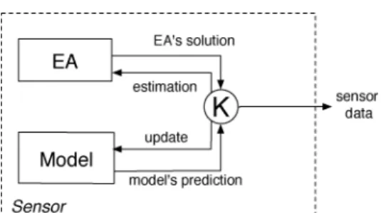
Figure 1: Improving the EA.

Figure 2: Standard filtering.

to them simply as thepredictionand itsaccuracy. Also, in order to improve readability, we shall omit hats and other subscripts or superscripts when there is no risk of confusion. We would like to point out that although filtering is a common practice in control systems engineering and tracking applications, the way we apply it is different. In a standard tracking application, filters like Kalman’s are used to have a good state estimation from the sensor information and the model. In our formulation the EA is part of the sensor, since it is the EA that actually provides the measurement, and filtering is used in order to improve the sensor’s accuracy by means of improving the EA’s behavior.

On top of the resulting sensor system, a more sophisticated tracking algorithm can be used, adopting some other filtering technique itself. Figures 1 and 2 illustrate the two solutions, where the circle “K” is the filtering technique adopted.

Finally, it is worth noting that the computational cost of the Kalman predictor is essentially due to matrix algebra and a matrix inversion (cf. Appendix A), which has a polynomial computational cost, and thus has little impact on the performances of the algorithms, assuming that the computational costs of the optimization process are dominated by the costs of evaluating the objective function.

3

Incorporating Motion Information

When Does Tracking Actually Begin? In particular applications, there might be a method to decide when the EA actually found a satisfactory optimum (e.g., fixing a fitness threshold), and to decide when tracking begins. In general, we do not have such information. Moreover, the estimator needs time to adjust: when can we start trusting it? The selection mechanism of the EA can be used to cope with this issue. The estimator will be started at the same time as the EA, providing almost useless predictions, and the individuals generated using them (see next section) will most likely be suboptimal and be discarded by the selection mechanism of the EA. While the EA evolves, the sequence of optima becomes more coherent, reflecting the fact that the algorithm got close to the optimum and began to follow it. Then, the predictions of the estimator will refine, and individuals incorporating them will take advantage of the information they carry.

Noise Can Make Observations Unreliable Noise can heavily affect the outcome of

the EA (depending on the application), and this in turn affects the input fed to the estimator. Although estimators like the Kalman filter are very good in dealing with noisy information (that is why they are called “filters”), we do not want to fully rely on them.

The Model Can Be Approximate For this reason, the estimator constantly needs real

observations in order to adapt to the real motion laws. Also, without constant update the estimator would not detect changes in the trajectory of the moving optima: the estimator needs new observations to keep refining. Moreover, the Kalman filter needs some tuning for optimal behavior. Since tuning is affected by a certain degree of approximation, we cannot fully trust its outcome.

Better Solutions Must Be Looked For The algorithm could be following a bad

opti-mum. Even in the tracking phase, there could be better solutions than the current EA’s best individual, close to it or in unexplored regions. Then, the algorithm has to be given the capacity to reach them, and not just focus on the current optimum. In other words, while the estimator is helping in the exploitationtask, a suitable degree of exploration must be ensured. This can only be provided by the EA.

The Moving Optimum Can Be Lost The EA can get stuck and not successfully follow

the optimum, for example because of noise in the input data, or because of a change of motion of the optimum not captured by the estimator’s model. If this happens, the algorithm must be able to recover tracking, and this can be achieved only by the EA’s exploration capabilities.

From the point of view of the EA, the motion estimator acts as anoracle, providing the future position ˆpt, that is, the new optimum’s position. Three techniques can be devised that allow for the addition of this kind of information into an EA.

• Modified genetic operators.In the basic version of EAs, genetic operators are blind,

in the sense that they do not make use of any problem specific information. This technique consists of the design of specialized mutation and crossover operations, that generate new individuals using some heuristic function that exploits the in-formation available. This category includes local search heuristic functions used to produce locally optimal (or near optimal) individuals.

• Modified fitness function. The fitness function is the place where all of the

Figure 3: Perturbation.

incorporated into the fitness function in the form of supplementary terms, called refining functions. Refining functions find use, for example, in discrete domains in order to help to discriminate between individuals with the same fitness.

• “Gifted” individuals.This technique consists of creating new individuals using the

information coming from the prediction, and inserting them directly into the pop-ulation. If the prediction was accurate enough, among these insertions will be the new optimum. In any case, such gifted individuals will spread the information they possess, mixing with the existing population in the subsequent generations.

Let us now describe in detail each of the three techniques listed above.

3.1 Modified Genetic Operators 3.1.1 Mutation

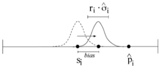
The mutation operator modifies one (or more) genes of a selected individual. Such mod-ification can be done by ignoring the previous value (new random gene), or performing some operation on the original value of the gene (perturbation), the simplest operation being adding or subtracting a small random quantity to the gene. Instead of using ran-dom quantities, the prediction can be used to bias the exploration, directing it toward the region where the new optimum will most likely be, according to the prediction (cf. Figure 3).

Letsbe the chromosome selected for mutation,sthe chromosome after mutation, andi∈1. . . nthe gene selected to be modified,nbeing the number of genes (chromo-some length). Let ˆpand ˆσ be the predicted position and its accuracy.

A common perturbation strategy is the Gaussian perturbationN(0, ri), centered in 0 and with a certain standard deviationri:

s_i=si+N(0, ri) (4)

where the parameterriis the range of the perturbation and can be either fixed at design time or computed according to some heuristic rule.

In our case, the perturbation should generate valuess_i close to the estimation ˆpi, depending on the accuracy ˆσi, and that are also in a range depending on the accuracy. A perturbation strategy that takes predictions into account will take the form

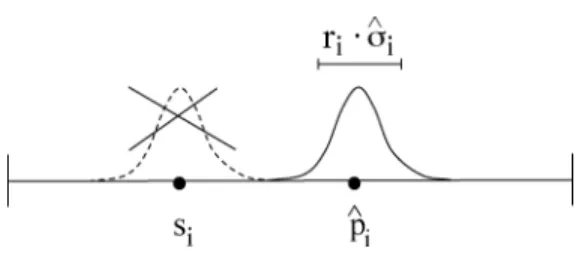
Figure 4: New random gene.

We propose to use the following heuristic function:

pert(ri,pˆi,σˆi)=bi × 1 1+σˆi

×( ˆpi−si)+N(0, riσˆi), 0< bi <1+σˆi, ri≥0 (6)

The first term is adirection bias(Figure 3) that determines the shift we want in the direction of the prediction. A bad prediction accuracy would produce a low bias: if the prediction is not accurate, it must not be taken into account. The second term determines the perturbation range, making it bigger or smaller according to the accuracy of the prediction.

The parametersbi andri control the bias and range values. Whenbi =1+σˆi, we have the maximum shift, whilebi =0 means no shift. Note that if ˆσi=0 andbi =1, the new gene will be exactly ˆpi (maximum confidence in the prediction).

A special case of this operator is obtained by setting the maximum shift. In this case the center of the perturbation will coincide exactly with the prediction, and the previous value of the gene will be ignored (Figure 4):

s_i=N( ˆpi, riσˆi). (7)

In the following, this case will be referred to as the new random gene mutation operator.

3.1.2 Crossover

The crossover operator searches the space by recombining the information of two existing individuals to generate new ones. The crossover operation does not imply the creation of new genetic material. One way to incorporate the prediction in the search performed by the crossover is to cross one individual selected from the population with one newly generated according to the prediction (see Section 3.3). In this way, the offspring will contain information regarding the prediction, and the search will be directed toward the point where the prediction indicates the new optimum will most likely be.

3.2 Modified Fitness Function

Adding refining terms to the fitness function is common practice for incorporating heuristic information into the evolutionary algorithm. Here, the idea is to privilege individuals that are close to the estimated future position, in order to help the algorithm to keep up with the moving optima, anticipating its movement.

Let s be the chromosome to be evaluated and f the base fitness function. The modified fitness function will beh:

h(s)=(1−a)×f(s)+a×r(s) 0< a <1 (8)

a simple heuristic being

r(s)= 1

1+σˆ_max × |pˆ−s|

where ˆσ_max= σˆ_∞is the maximum of the ˆσi.1The refining termr(s) takes into account the distance from the estimated future position, and weights it with the confidence we have in the prediction: the higher the confidence (small ˆσ_max), the higher the penalty for being far from the predicted position. The parametera is used to tune the relative weight of the refining function, and will depend on the problem under study.

3.3 Gifted Individuals

This technique consists of generating a certain number of new individuals, using the information coming from the estimator. In principle, if the estimator were perfect, we could just generate one new individuals=pˆ and this would correspond to the new optimum. In general, since the estimation is not perfect, the new optimum is likely to be in a neighborhood of ˆp, whose size is estimated by ˆσ. Thus, the idea is to generate some individuals in that neighborhood.

LetP be the population size, and 0< g <1 the proportion of population we want to be composed of new gifted individuals. Then, a number of gPindividuals will be generated in the neighborhood of the prediction (si=N( ˆpi,σˆi), i=1. . . n) and the remainingP − gPwill be generated in a standard way. The caseg=0 would mean rejecting the prediction, the caseg=1 would mean to reject the whole old population and create a new one, in the neighborhood of ˆp.

In the same way we have done before, a simple heuristic rule is thatgshould be inversely proportional to ˆσ_max: the less confident we are in the prediction, the fewer individuals we generate following it.

g= c

1+σˆ_max, 0< c <1+σˆmax (9)

The main difference between the gifted individuals technique and the modified operators technique is that gifted individuals are generated from scratch, and do not make explicit use of the existing genetic material, while the genetic operators generate

1_{Since each gene has its own ˆσ}

Table 1: Summary of the Techniques

Technique Parameters Range Heuristic

New random gene — — —

Biased perturbation biasb 0< b <1+σˆi ₁₊1_σˆ

i( ˆpi−si)+N(0,σˆi)

Single parent crossover — — —

Refining function weighta 0< a <1 1

1+σˆmax|pˆ −s|

Gifted individuals proportionc 0< c <1+σˆmax 1/(1+σˆmax)

Figure 5: Geometry of the problem.

new individuals modifying existing ones. Hence, in the first case the new genetic material will mix with the existing material in a future time.

Table 1 summarizes the characteristics of the techniques described above.

In order to perform an experimental assessment of the techniques described above, we have applied them to a practical application known as the pose problem, which we present in the next section.

4

The Pose Problem

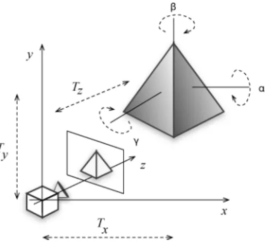
Consider a scene composed by a three-dimensional world in which an object is seen by a camera, projected into a two-dimensional plane. Figure 5 shows the coordinate system of the space where the object is placed.Tx,Ty andTzare the translation values with respect to the camera (positioned in the origin of the axes), and α,β,γ are the rotation angles about each axis.

The pose problem is in fact a dual problem: establishing a correspondence between image features and model features, and finding the rotation and translation of the object with respect to the coordinate system. Each problem is easy to solve if the other has been solved first. Given the matching between model and image features, one can determine the pose that best aligns those matches. If the object pose is known, one can easily determine such matches, projecting the model with the known pose into the original image. The complete (pose and correspondence) problem is difficult because it requires the solution of two coupled problems.

The problem of pose estimation is central in computer vision, and has been ap-proached with a variety of methods, such as Neural Networks (Wunsch and Hirzinger, 1996) and linear programming (Lowe, 1991). One of the most complete algorithms that deal with the correspondence and pose estimation simultaneously is SoftPOSIT (Davids et al., 2002). For a comprehensive survey of different techniques of three-dimensional object modeling, correspondence, and pose estimation Faugeras (1993) and Horaud et al. (1997) are recommended.

4.1 Evolutionary Pose Estimation

The pose estimation problem can be formulated as an optimization problem in the following way (Rossi et al., 2005b).

We have to find the value of the six parameters (Tx, Ty, Tz) that give the position with reference to the camera position, and (α, β, γ) that represent the orientation of the object (see Figure 5). If such parameters are given, let them beso_=(To

x, Tyo, Tzo, αo, βo, γo), then rotating and translating the model object by the corresponding values, and projecting it into the camera plane, would result in a perfect match between camera image and model projection. In this case, the sumdof the distances between each pair of corresponding points would be zero.

If one parameter, corresponding to one dimension, differs from the correct value, for exampleTx =Txo+, then each projected pointmiof the model would be shifted by a quantityfi() with respect to the corresponding point in the camera image,fi being functions that depend on the geometry and camera settings. The sum of the distances in this case would bed =_i|fi()|. The closer the projections=(Tx, Ty, Tz, α, β, γ) to the camera image, the smaller isd. Being thatso_{is unknown, the only way to compute} d is by measuring the distance between image points and projected model points, and search for a solutionssuch thatdis minimized. The matching problem is then turned into an optimization problem:

min(d =_i|pi−mi(s)|), pi, mi∈IR2

s=(Tx, Ty, Tz, α, β, γ)

(10)

where pi is a point in the image,mi(s) is the model point projected according to the set of parameterss=(Tx, Ty, Tz, α, β, γ), andis the Euclidean distance between two points. Since the correspondence between points is not known in advance, we consider a projected model point to match an image point if it is the closest. Thus, the distance measure becomes:

d= i

Figure 6: Distance and matching points.

Figure 6 shows an example where two different sets of parameters sM _{and s}N lead to two different sets of projected model points, set M= {m₁, m₂, m₃, m₄}and set

N = {n₁, n₂, n₃, n₄}. The point correspondence is shown with dashed lines. The distance between the points of setMand the image pointsP = {p₁, p₂, p₃, p₄}is clearly smaller than the total distance of pointsNfrom pointsP. Therefore, the setMis a better match and the corresponding set of position parameterssM _{is a better solution.}

If some of the points are noisy, the minimum total distance d will not be zero. This fact can affect the optimum solution, depending on the level of noise. If noise is limited, the minimum distance in most cases still relates to a good point matching, as the perturbation affects bothsM _andsN_{. This is shown in Figure 6, where pointp}

2 is moved top₂: although the total distance is changed, setMstill matches better than set

N. The same situation occurs when some of the points in the image are missing or are added (false positives) due to poor image quality, partial occlusions, and/or to faults in the feature extraction process.

Nevertheless, noise can affect the optimum solution in two ways. First, the optimum solution can change, especially when two (or more) solutions are similar, and the noise benefits the “wrong” one. In this case the minimum distance does not correspond to the real pose of the object, but to a slightly different pose, and the precision of the solution is affected. Second, the objective function can present local minima, especially in the presence of a high number of false positives spread in the image. A local minimum appears when there is a subset of image points that produce a small total distance with the model projected according to a given set of parameters, while the set of parameters does not correspond to the correct pose. For this reason it is important to rely on search methods capable of overcoming local optima such as EAs, where a search is done by sampling the solutions space.

In the EvoPose algorithm, the arrays is a candidate solution, encoded as a six-dimensional array of real numbers, and a good solution is sought with an evolutionary algorithm that maintains a population of candidate solutions and evolves them toward optimality by means of the genetic operators.

Figure 7: Matrix algebra of the rotation/translation/projection operation.P is the per-spective projection matrix and depends on the camera properties, R is the rotation matrix. The final bidimensional coordinates in the image are (x/w, y/w).

Equation 11). This makes the scale-up behavior of the algorithm suitable for real images, where hundreds of points may need to be considered.

4.2 Moving Objects

The problem of tracking a moving object consists of determining the pose of the object in a sequence of images, where the position and/or orientation of the object vary in time. Once the pose of the object has been determined for an image, one can use this information in order to determine the position of the object in the following image, without having to solve from scratch the pose problem for the new image.

When dealing with moving objects in a sequence of images, the set of image points

P = {pi} changes in time, becomingP(t)= {pi(t)}. Thus, the distance function from Equation 11 becomes a function of time:

d(t)= i

minj(|pi(t)−mj(s)|) (12)

In our search problem, this means that we have atime-varyingfitness function. Note that as new candidate solutions are generated searching in the neighborhood of the best existing individuals in the population, the information about the previous position is actually used in order to find the new one.

Figure 8 shows an example of the distance from the target points of the best solution in the case of rotation around one axis (see Section 5 for more details). The behavior is less smooth for higher speeds. Also, the distance increases as the speed of the object increases, since it takes longer for the GA to find the new position if this is far from the previous one. Table 2 reports the results corresponding to Figure 8. The column 2nd

halfis the most interesting to our purposes, since it refers to the tracking phase of the run.

5

Experimental Results

Figure 8: Average distance comparison (rotation around vertical axis).

Table 2: Comparison of Average Distance:Is the Angle Increment for Each Genera-tion, Over the Chromosome Domain [0,1]

Speed Average distance

(/gen) 1st_{half 2}nd_{half Overall}

0.001 0.0463 0.0072 0.0267

0.002 0.0711 0.0237 0.0474

0.005 0.1421 0.0800 0.1109

0.0075 0.2163 0.1346 0.1758

0.010 0.2160 0.1605 0.1879

In order to eliminate external factors, synthetic images have been used. At each gen-eration, the pose of the the target object (optimum solution) was updated as described below, and a new frame was generated with the target object in the corresponding position and orientation. Then the new frame was processed in order to detect the corner points, and the new set of points was used to compute the distance function in Equation 12. In the detection step noise, for example, false positives, can appear (cf. Figure 9, right).

The domain of the genes was [0,1], while the phenotype range was [0,500] forx

and y positions (frame size of 500×500 pixels), [0,1] for the distance z, and [0,2π] for rotation. The cube size was 35 pixels. Hence, a value of, for example, =0.001, actually meant a speed of the cube of 0.5 pixels/generation for translations and a rotation speed of 0.36 deg./generation. The rotation experiments have been performed at slower speeds with respect to translations, since the genotype range of the rotation parameters maps in a much smaller phenotype range, resulting in higher rotation speed.

Figure 9: An image of the target object (left) and of the points extracted by the feature-extraction process (right). In this example, seven corners were correctly de-tected (squares), one point was missing because it was hidden (empty circle), and two false positive points were detected (filled circles).

to position or orientation was given varying values from 0.1 to 0.9 with increments of

at each generation, and the remaining genes were assigned random values. The limits were chosen to avoid the boundaries of the domain.

5.1 Evolutionary Algorithm

The evolutionary algorithm settings have been set as follows:

• Type: generational. Population size: 100 individuals. • Selection: standard roulette.

• Representation: array of six real valued genes in the domain [0,1].

• Crossover: standard one point crossover (except when the SINGLE-XOVER oper-ator is applied). Rate: 0.5.

• Mutation: Gaussian random perturbation (except when operators (5) and (7) are used). Rate=0.9, Rangeri=0.1 (10% of the domain).

This kind of evolutionary algorithm has been chosen because of its simplicity and because its working principles are well understood. Moreover, it allowed for easy incorporation of the different techniques described earlier. The setting of the parameters has been chosen during early testing on the basis of the EA’s good performances. We believe that such choices have little influence on the main focus of the paper.

5.2 Performance Measure

The goodness of an algorithm is measured with the average distance of the best in-dividual from the real position. This measure is similar to the offline performance

Figure 10: Example of the behavior during the early stage of the search: distance from the optimum of the best individual (=0.005).

Branke (1999; see also Jin and Branke, 2005). In our case, the average is computed using the total number of generations, while f_offline is computed using the total number of evaluations.

Since we are interested in the tracking performances and there is no way to dis-criminate between initial search and tracking, we will focus the analysis on the second half of the runs, when we suppose the algorithm has found the object and is following it. In order to compare the “smoothness” of the runs, we take into consideration the mean standard deviation of the distance over a run.

5.3 Discussion

Figures 10 and 11 show an example of the behavior of the different techniques in the early stage of the search. During the very first iterations it can be observed that the plain EA performs slightly better than the versions incorporating the predictions, since the prediction mechanism has not been refined yet, and its estimations are useless. The same behavior can be observed in Table 3, where the average number of evaluations needed to find the first good solution in the case of a stationary object is reported.

Figure 11: Comparison of all strategies in the first half of the run: average distance from the optimum.

Table 3: Number of Evaluations Needed to Obtain a Good Pose (Stationary Object)

Plain EA 1,962 Single parent crossover 2,484

New random gene 3,857 Refining function (a=0.5) 3,058 Biased perturbation (b=1.0) 3,490 Gifted individuals (c=0.1) 3,922

.

Figure 12: New random gene.

Figure 13: Biased perturbation.

Figure 14: Single-parent crossover.

which is an essential feature in dynamic optimization. In fact, a spread-out population adapts easily to changes in the environment. In order to maintain an adequate degree of diversity in the population, besides incorporating more sophisticated diversity control techniques, some action can be taken, such as using small values for the parameter of the various strategies, using larger populations, using high rates for the genetic operators, or adopting more disruptive operators.

Figure 15: Refining function.

Figure 16: Gifted individuals.

the differences between the five techniques are not significant.2 _{For low speeds the} difference between the plain evolutionary algorithm and the different techniques is not significant, while it becomes significant with increasing speeds. Table 4 reports the average and standard error corresponding to the experiment, for the case =0.01. Figure 18 shows a comparison between the average standard deviation of the distance over a run of the best of each technique. In this case the single parent crossover and the biased mutation seem to be best, except for one case (=0.01).

Figure 17: Translation: comparison of all strategies.

Table 4: Detailed Data for Figures 17 and 19: Average and Standard Error of the Dis-tance for=0.01

Translation Rotation

Technique Average Standard Error Average Standard Error

Plain EA 0,02192 0,00320 0,16158 0,02278

New random gene 0,00815 0,00109 0,10036 0,02713

Biased perturbation 0,00904 0,00078 0,08581 0,02657

Single parent crossover 0,00705 0,00100 0,10058 0,02646

Refining function 0,00799 0,00074 0,09184 0,02851

Gifted individuals 0,00922 0,00103 0,10567 0,02458

Figure 19: Rotation: comparison of all strategies.

Figure 20: Rotation: average standard deviation of the distance over a run.

The results for rotation are similar to the ones for translation, and the improved versions of the algorithm still outperform the plain version in a significant way for high speeds (cf. Table 4). The modified crossover operator still appears to be the best performing, together with the modified mutation operator. However, and this is also true for rotations, the differences between the proposed techniques have not been found significant. The results for the test on rotation are summarized in Figure 19, which shows a comparison between the best of each technique.

Figure 21: Behavior of standard deviation of the prediction (accuracy).

same (constant increment of the value of a gene), the way a change in the gene affects the phenotypes is different. In case one of the genes encoding the position changes, the induced change in the genotype results in a translation in the position that does not change the relative distance between the projected model points, as they are all shifted by a quantity depending on the distance and focal length. Hence, changes in the genotype are reflected monotonically in the phenotype. In case one of the genes encoding the orientation changes, the induced change in the genotype results in a rotation of the object. Thus, the relationship between a change in a gene and the corresponding change in the phenotype is of a trigonometric nature. In rotations, the relative positions of the points change: points can get closer, farther, or overlap, and points can appear and disappear according to the point of view of the observer.

5.3.1 Accuracy

Figure 21 depicts the behavior of the standard deviation of the prediction, that is, the prediction’s accuracy. The accuracy has the same behavior for both rotation and translation, since the same fixed initial values and error covariance were used (cf. Appendix A). Starting from the default value of 1, it rapidly increases, due to the high variances used as initial values for the measurement process (outcome of the EA), to reflect the initial highly varying outcome of the evolutionary algorithm. For simplicity, such values have been estimated off-line in early testing of the algorithm, but they can be computed online on the basis of the actual behavior of the algorithm.

During the run, the predictor is refined and its error drops to stabilize to a value of around 0.4. When used in the heuristic rules in Equations 6 and 7 it generates for the perturbation rangeri·σˆi, values as high as 0.57 in the early stage of the search, that later self-adjust to 0.04, while the plain algorithm uses a default value ofri =0.1 throughout the whole run.

Figure 22: Object moving in four dimensions (first 100 generations,=0.002, average over 50 runs).

Table 5: Average and Standard Error of the Mean Fitness in the Second Half of the Run, Object Moving in Four Dimensions,=0.002, Average Over 50 Runs

Technique Average Standard Error

Plain EA 40,913 2,717

New random gene 29,618 2,740

Biased perturbation 31,703 2,759

Single parent crossover 29,191 2,538

Refining function 13,606 0,895

Gifted individuals 24,132 3,900

5.3.2 More Complex Motion

Figure 22 shows the performance of the different strategies when four variables are changing, two for translation and two for rotation: the target object is moving in diagonal and rotating around two axes. In this test, in order to increase significance, 50 runs have been performed for each technique.

In the case of combined motion, the algorithm exhibits a behavior similar to the one described earlier, when the case of only one changing variable was analyzed. All the proposed techniques perform better than the plain evolutionary algorithm, while the differences between them are not significant, with the exception of the refining function technique. The latter shows better performance, with a significant difference compared to the other techniques.

Table 5 reports the average and the standard error of the fitness corresponding to the test. The values in the table are the average and standard error over the 50 runs of the mean fitness of each run, computed taking into account the second half of the run (note that Figure 22 shows only the first 100 generations, while a complete run lasts 400 generations).

Figure 23: Linearly changing speed,₀=0.01,δ= −0.00005.

object has been decreased linearly during the run, starting from a value of₀, modified at each step by adding a valueδ. The values ofδwere chosen in such a way to cause a change of the direction of the movement.

For low speed and slow changing rate no significant differences could be observed, indicating that the model successfully adapted to the changing environment, and the effectiveness of the algorithm was not compromised. However, for a higher speed and changing rate, differences start to emerge, depending on the prediction incorporation technique adopted. Figure 23 shows example runs of such differences. The most critical moment appears to be the change of direction. Around this point is where the highest differences can be observed. In particular, the two biased mutation operators encounter difficulties after the change in the direction of the movement, and the algorithms adopt-ing them show a significant delay in followadopt-ing the movadopt-ing optimum.

Experiments performed with different settings of the parameters (not reported here) confirm that the limitations of the proposed approach are due to the filter failing to adapt to the motion law, when this is different from the model used. Nevertheless, even an approximate model can provide useful predictions by dynamically adapting to the observation, when changes are sufficiently small. Extensive simulations will be the object of future work.

6

Conclusion

The learning and prediction mechanism we adopted is based on Kalman filters. Although filtering is a common practice in control systems engineering and tracking applications, the way we apply it is different, since in our formulation filtering is used in order to improve the EA’s behavior, and not as a more post-processing tool, which is the common practice.

The experiments conducted on a well-known computer-vision problem indicate that the predictions actually help to improve the tracking of the moving optimum, both in terms of average distance to the real position and smoothness of the tracking. Due to its nature, the learning and prediction mechanism has negligible impact on the performance as far as the computational cost is concerned.

Experiments also indicate that prediction mechanisms are helpful in order to im-prove the tracking capabilities of an evolutionary algorithm, but they must not be overestimated because they can lead to an excessive convergence, which has a negative impact on the algorithm, as indicated by several works in the literature. Coupling pre-dictions with some diversity control technique can be a promising strategy for taking advantage of the improved exploitation capabilities provided by the predictor, while maintaining a suitable degree of exploration. The biased mutation operator has shown better overall performance for the case of simple motion, but there is no clearly winning strategy. Each technique has its own characteristics and which technique performs best may depend on the problem at hand. Future work will be aimed at investigating the peculiarities of the different strategies.

The main disadvantage of the proposed approach is that in some cases an additional parameter is introduced that controls the effect of the predictions on the algorithm. Also, the kind of prediction algorithm we adopted needs an off-line tuning prior to its application, in order to estimate initial parameters (noise covariance). However, such parameters can be computed online based on the actual behavior of the algorithm.

We did not investigate the effect of different choices of the evolutionary algorithm parameters such as population size, selection rule, type of algorithm, etc. Nevertheless, we believe that the insight provided by the experiments performed allows us to draw the conclusion that the idea can be effectively applied to other kinds of evolutionary algorithms and applications, and it is not limited to Kalman-based estimators but it can be extended to any other problem specific learning algorithm and to any other problem specific state transition (motion) law.

Acknowledgments

The work of the first and second authors has been carried out under a “Ramon y Cajal” research fellowship from the Ministerio de Ciencia y Tecnolog´ıa of Spain, and partially funded by projects DPI2005-04302 and DPI2006-03444.

Appendix A Kalman Filters

The Kalman filter estimates a system by using a feedback control: the filter estimates the process state, and then obtains feedback in the form of (noisy) measurements. The kind of dynamic system considered by Kalman filters is the following;

xt =Axt₋1+Cut₋1+wt₋1,

where xt ∈IRn is the state of the system at time t, A is the state transition model (n×n matrix) and C is an optional control input model. The value zt∈IRm is the observation of the system (measurement) at time t andH ∈IRm×n _{is the model that} relates the measurement to the state, since all variables of the state are not necessarily being observed: in our case we only measure position, while the state also contains velocities. The quantitieswandvare random variables that represent the process and measurement noise, and are assumed to have a Gaussian distribution with covariance matricesQ∈IRnandR∈IRm, respectively (p(w)∼N(0, Q), p(v)∼N(0, R)).

The model provides an a priori estimation of the new statex_t−. The new state is computed correcting the a priori estimation with the real observationzt through the Kalman gain matrixKt ∈IRn×maccording to the formula:

ˆ

xt =xt−+Kt(zt−H xt−)

The gain matrix is computed recursively and balances the two terms x_t− and zt according to their respective covariance.

To begin to work, the filter needs an initial statex₀, an initial error covariance matrix

P₀, usually set to a default value, and the matricesQandR, usually measured during the early testing of the system.

Then, the filter loops through a series of steps. The first step is to generate the a priori estimate using the model and to calculate the a priori error covarianceP_t−. The a priori estimation and the a priori covariance provide the values we refer to as the

predictionand itsaccuracythroughout the paper.

Next, the measurement update phase takes place, first computing the Kalman gainKt. The matrixKtis computed in such a way that minimizes the a posteriori error covariancePt. The next step is to actually measure the process (obtain the observationzt), and then to generate an a posteriori state estimatextby incorporating the measurement, which is the estimation usually employed in practical applications (cf. Figure 2). The final step is to obtain an a posteriori error covariance estimatePt. Note how the corrected values forxtandPtwill be used in the next time step to predict the new state and its error, hence the model actually incorporates the information coming from the measurement to correct its predictions and adapt to the measurements.

In our case,xt=St =[pt, vt], and the model given in Equation 2 can be rewritten according to Equation 13:

xt =Axt−1, A=

I t·I

0 I

(14)

I being the 6×6 identity matrix and there is no control input, that is,C=[0].

References

Angeline, P. J. (1997). Tracking extrema in dynamic environments. In Angeline, P. J., Reynolds, R. G., McDonnell, J. R., and Eberhart, R. (Eds.), International Conference on Evolutionary Programming(pp. 335–345). Berlin: Springer Verlag.

Arnold, D. V., and Beyer, H.-G. (2006). Optimum tracking with evolution strategies.Evolutionary Computation, 14(3):291–308.

B¨ack, T. (1998). On the behavior of evolutionary algorithms in dynamic environments. In Fogel, D. B., Schwefel, H.-P., B¨ack, T., and Yao, X. (Eds.),IEEE International Conference on Evolutionary Computation(pp. 446–451). Piscataway, NJ: IEEE Press.

Beyer, H. G. (2001). The Theory of Evolutionary Strategies. Natural Computing Series. Berlin: Springer-Verlag.

Bosman, P. A. N. (2005). Learning, anticipation and time deception in evolutionary online dy-namic optimization. InFourth Workshop on Evolutionary Algorithms for Dynamic Optimization Problems (EvoDOP-2005), pp. 39–47.

Branke, J. (1999). Memory enhanced evolutionary algorithms for changing optimization prob-lems. In Angeline, P. J., Michalewicz, Z., Schoenauer, M., Yao, X., and Zalzala, A. (Eds.), Congress on Evolutionary Computation, vol. 3 (pp. 1875–1882). Piscataway, NJ: IEEE Press.

Branke, J. (2001). Evolutionary approaches to dynamic optimization problems. In Branke, J., and B¨ack, T. (Eds.),Evolutionary Algorithms for Dynamic Optimization Problems(pp. 27–30).

Branke, J., Kaußler, T., Schmidt, C., and Schmeck, H. (2000). A multi-population approach to dynamic optimization problems. InAdaptive Computing in Design and Manufacturing 2000, pp. 299–308.

Cedeno, W., and Vemuri, V. R. (1997). On the use of niching for dynamic landscapes. InCongress on Evolutionary Computation(pp. 361–366). Piscataway, NJ: IEEE Press.

Cobb, H. G. (1990). An investigation into the use of hypermutation as an adaptive operator in genetic algorithms having continuous, time-dependent nonstationary environments. Technical Report AIC-90-001, Navy Center for Applied Research in Artificial Intelligence, Washington, DC.

Davids, L., DeMenthon, D., Duraiswani, R., and Samet, H. (2002).SoftPOSIT: Simultaneous pose and correspondence determination. InEuropean Conference on Computer Vision, vol. 3 (pp. 698–703).

De Jong, K. A. (1975).An analysis of the behavior of a class of genetic adaptive systems. Unpublished doctoral dissertation, University of Michigan, Ann Arbor.

Faugeras, O. (1993). Three-dimensional computer vision: A geometric viewpoint: Cambridge, MA: MIT Press.

Grefenstette, J. (1992). Genetic algorithms for changing environments. In M¨anner, R., and Mand-erick, B. (Eds.),Parallel Problem Solving from Nature(pp. 137–144). New York: Elsevier Science.

Hansen, N., and Ostermeier, A. (2001). Completely derandomized self-adaptation in evolution strategies.Evolutionary Computation, 9(2):159–195.

Horaud, R., Dornaika, F., Lamiroy, B., and Christy, S. (1997). Object pose: The link between weak perspective, paraperspective, and full perspective. International Journal of Computer Vision, 22(2):173–189.

Jin, Y., and Branke, J. (2005). Evolutionary optimization in uncertain environments—A survey. IEEE Transactions on Evolutionary Computation, 9(3):303–317.

Lowe, D. (1991). Fitting parameterized three-dimensional models to images. IEEE Transactions on Pattern Analysis and Machine Intelligence, 13(5):441–450.

Mori, N., Imanishi, S., Kita, H., and Nishikawa, Y. (1997). Adaptation to changing environments by means of the memory-based thermodynamical genetic algorithm. In B¨ack, T. (Ed.), International Conference on Genetic Algorithms(pp. 299–306). Piscataway, NJ: IEEE Press.

Ostermeier, A., Gawelczyk, A., and Hansen, N. (1994). Step-size adaptation based on non-local use of selection information. In Davidor, Y., Schwefel, H.-P., and M¨annerm, R. (Eds.),Parallel Problem Solving from Nature(pp. 189–198). Berlin: Springer-Verlag.

Ramsey, C. L., and Grenfenstette, J. J. (1993). Case-based initialization of genetic algorithms. In Forrest, S. (Ed.),International Conference on Genetic Algorithms(pp. 84–91). Piscataway, NJ: IEEE Press.

Rossi, C., Abderrahim, M., and Diaz, J. (2005a). An evolutionary algorithm for model-based object pose estimation and tracking. InIEEE International Conference on Visual Information Engineering, pp. 78–83.

Rossi, C., Abderrahim, M., and Diaz, J. (2005b). Evopose: A new model-based pose estima-tion algorithm with correspondences determinaestima-tion. In IEEE International Conference on Mechatronics and Automation 2005, vol. 3, pp. 1551–1556.

Stroud, P. D. (2001). Kalman-extended genetic algorithm for search in nonstationary environments with noisy fitness evaluations.IEEE Transactions on Evolutionary Computation, 5(1):66–77.

Vavak, F., Fogarty, T. C., and Jukes, K. (1996). A genetic algorithm with variable range of local search for tracking changing environments. In Voigt, H.-M., Ebeling, W., Rechenberg, I., and Schwefel, H.-P. (Eds.),Parallel Problem Solving from Nature(pp. 376–385). Berlin: Springer.

Weicker, K., and Weicker, N. (1999). On evolution strategy optimization in dynamic environ-ments. In Angeline, P. J., Michalewicz, Z., Schoenauer, M., Yao, X., and Zalzala, A. (Eds.), Congress on Evolutionary Computation, vol. 3 (pp. 2039–2046). Piscataway, NJ: IEEE Press.