DOI: 10.13164/re.2016.0409 FEATURE ARTICLE
Stability Analysis and Design of Negative Impedance
Converters: Application to Circuit and Small Antennas
Daniel SEGOVIA-VARGAS
1, José Luis JIMÉNEZ-MARTÍN
2, Ángel PARRA-CERRADA
2,Fernando ALBARRACIN-VARGAS
1, Eduardo UGARTE-MUÑOZ
1,Vicente GONZALEZ-POSADAS
21 Dept. of Signal Theory and Comm., Carlos III University of Madrid, Av. La Universidad 30, 28911, Leganés, Spain 2 Dept. of Audiovisuals and Comm., Polytechnic University of Madrid, Km 7 Valencia-Highway, 28031 Madrid, Spain
[email protected], [email protected], [email protected]
Manuscript received June 2, 2016
Abstract. Negative impedance converters (NICs) have been proposed as structures to improve the performance of RF circuits and electrically small antennas. However, NICs suffer from stability problems. This paper presents a com-pact procedure to analyze the stability of NICs. Then, the required and sufficient conditions to predict the stability of a negative impedance converter are given. These condi-tions can be evaluated using standard computer-aided-design software. Finally, a NIC prototype is given to vali-date and illustrate the presented design procedure, it is also integrated with a printed, blade-type, electrically small monopole in the VHF band.
Keywords
Negative Impedance Converter (NIC), stability, network Nyquist test, electrically small antennas
1.
Introduction
Negative Impedance Converters (NIC) are electronic circuits that can provide new possibilities for radio-fre-quency and microwave circuits [1–4]. NICs can be used to increase the bandwidth of matching networks (MN), espe-cially if they are realized on integrated or monolithic tech-nologies (RFIC/MMIC). The NIC is a two-port network that, at port one, gives a negative, and possibly scaled, version of the impedance loading the port two; and vice versa.
The use of NICs can offer multiple possibilities to the circuit or system where they are integrated. Firstly, they can compensate the inductance or the capacitance to in-crease the impedance matching bandwidth of the circuit. Secondly, in parallel or series RLC circuits resonant cir-cuits, negative capacitors or negative inductors can be used to modify the resonant frequency and the quality factor Q. Finally, negative resistors or negative conductances G can be used to improve the Q factor without modifying the resonant frequency.
One of the biggest drawbacks associated with the use
of NIC circuits, at microwave frequencies, is their inherent stability problems. Several papers dealing with the circuit stability can be found [5–11]. All these methods are based on the Nyquist criterion to check if the corresponding net-work function does not have any poles lying in the right-half of the complex plane (RHP).
The analysis of the stability of any microwave system requires both the study of a corresponding transfer function and the modeling of the inside active elements. Linear modeling of active circuits is preferred because of its speed and simplicity. Non-linear modeling requires both a heavier computational cost and accurate non-linear models of the active devices that are not always available [5–12]. For those reasons, when the corresponding network function is a suitable tool, and under some conditions [13], linear simulations can be used to research new design topologies using the S parameters of the active element.
Classic linear methods for NIC analysis can be classi-fied in two groups: those related with the impedance, ad-mittance or reflection coefficient function at the NIC output [6–10] and those related with the analysis of the open-loop gain in a two-port network [11], [14].
verters are still completely open and more attention should be paid on them. In [20], [21] and [22], a new function for the stability analysis was proposed as a suitable tool to be used in the amplifier stability study. According to [21], the so-called normalized determinant function (NDF) allows using linear modeling for providing accurate methods to analyze the stability and performance of amplifier circuits. This paper proposes to use the NDF to analyze much more complex circuits such as negative impedance converters (NICs). In this method, the NIC is considered as a poten-tially stable device. Then, the goal is to find out which load and source impedances make the NIC stable. It must be emphasized that it is not only necessary to see which load impedance ZL is negated, but also study how does the
source impedance ZS affect the NIC loaded with ZL. Other
passive components in the system can also be included in the stability analysis, in this sense, a practical design ex-ample where the NIC is used as an embedded broadband matching network in an electrically small antenna (ESA), is presented in order to apply the NDF method for predicting the stability of the overall system: antenna + MN.
The paper is organized as follows. Section 2 presents a critical study for the classic linear methods to analyze NICs in order to see its validity and shows the need of additional conditions for stability. In Sec. 3, a general method based on the normalized determinant function is presented. This method will allow us to study, in a general and an accurate way, the stability of the NIC circuits. Sec-tion 4 states the addiSec-tional condiSec-tions that the methods presented in Section 2 must satisfy in order to be valid for a proper prediction of the stability. These additional condi-tions are based on the aforementioned NDF method. Then, to show the potential of the NDF, a practical design exam-ple is presented in Sec. 5. Finally, Section 6 gives the con-clusions.
2.
Linear Methods for Studying
Stabil-ity in NICs
Two different kinds of methods are being used to analyze the NIC performance in this section: the reference plane methods and the loop gain method.
2.1
Reference Plane Methods
Concerning the reference plane methods, it was stated in [6] that the necessary condition for stability, at the input or output port when the other port was open or short-cir-cuited, was that its corresponding impedance Z(s) or admittance function Y(s), respectively, had not any poles in the RHP, in other words, the real part of the one-port cir-cuit function must be positive. There is a lack of con-sistency in the previous statement since there is not any comment on the actual loads to be inverted – capacitors and inductors; in addition, the active elements are considered as ideal ones leading to inaccurate results.
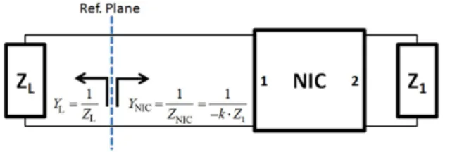
Fig. 1. Schematic of the NIC for a one-port network.
In a later approach [1], it was tried to generalize the previous criterion by considering any impedance or admit-tance to be inverted. A similar analysis was undertaken by considering the one-port network shown in Fig. 1. Then, the so called “open circuit stable” (OCS) condition states that the necessary, but not sufficient condition, for the NIC stability is that the absolute value of the impedance at port 1 (ZL in Fig. 1) should satisfy the following condition for
all frequencies at which the NIC can effectively work.
L IN = NIC or L IN = NIC OCS port
Z Z Z Y Y Y . (1)
While for the “short circuit stable” (SCS) condition, a necessary, but not sufficient condition for the NIC stabil-ity is that the absolute value of the admittance at port 1 YL
should satisfy the following condition for all frequencies at which the NIC can effectively work.
L IN = NIC or L IN = NIC SCS port
Y Y Y Z Z Z . (2)
For these reasons, the previous condition cannot as-sure the stability of the NIC device by itself, since it does not take into account the locus with frequency of the trace of the corresponding network function.
2.2
Loop Gain Methods
When the NIC is considered as a feedback system loaded with ZL and ZS. The goal is to find out a set of
val-ues for ZL and ZS that makes the NIC stable. This method
has been traditionally applied by the oscillator theory. If the NIC is considered as a feedback system, the lack of oscil-lating conditions makes the NIC stable. According to Fig. 2 the general network function is given as
o i
( ) ( )
1 ( ) ( ) G s
X s X s
G s H s
. (3)
where Xo(s) and Xi(s) are the corresponding output and
input functions (i.e. current or voltage) while G(s) and H(s) are the forward and reverse gain functions. The parallel-series feeding-back is used for NICs because one port is an impedance port while the other one is an admittance one.
Fig. 2. Schematic of the NIC based on a feedback topology.
Another loop-gain method is presented in [24], where the closed-loop gain function was defined by the ratio be-tween its input and output currents since any feedback system can be decomposed in a two-port network con-nected in closed loop (see Fig. 3). Then, the closed-loop transfer characteristic based on the Z or S-parameters can be taken out as follows:
o 21 11 22 11 21 12 21 11 22
11 12 21 22 12 21 12 21 11 22
2 1
1 ( )
I Z Z S S S S S S S
I Z Z Z Z S S S S S S
(4) where the Z and S parameters are the ones obtained from
the two-port network being I the input current and Io the
output current.
Assuming that the S-parameters do not present poles in the RHP, the stability of the NIC would be given by the existence of zeroes in the RHP of the denominator of the function Io/I.
Another alternative consists of using an open-loop gain function, instead of the close-loop gain function. The open-loop gain function can be obtained by opening the feedback loop at any point and applying the virtual ground technique [24]. Then, a new open-loop gain function GL
can be rewritten in terms of the S-parameters as in [24]:
21 12 21 12
L
11 22 2 12 1 11 22 12 21 2 12
Z Z S S
G
Z Z Z S S S S S
(5)The main advantages of this GL function are its
invariance with the opening point and that it does include the mismatching effect at the connection point. If GL = 1,
the root-loci of the GL function define the existence of
a pair of complex poles depending on how it encircles the +1 point. The system will be stable if the locus does not clockwise encircle the +1 point. It is important to remark that GL= 1 is satisfied whenever:
Fig. 3. Diagram of the NIC for calculating the currents ratio.
(a) (b)
Fig. 4. (a) A classic NIC topology to convert C2 where
C1 = 5 pF, R = 495 Ω, L = 5 nH, C2 = 2 pF, Q1= Q2= BFR360F, VCE = 3 V, IC = 10 mA. (b) The modified topology to analyze its stability with the closed loop gain function.
Fig. 5. Detail of the root-loci of the GL function.
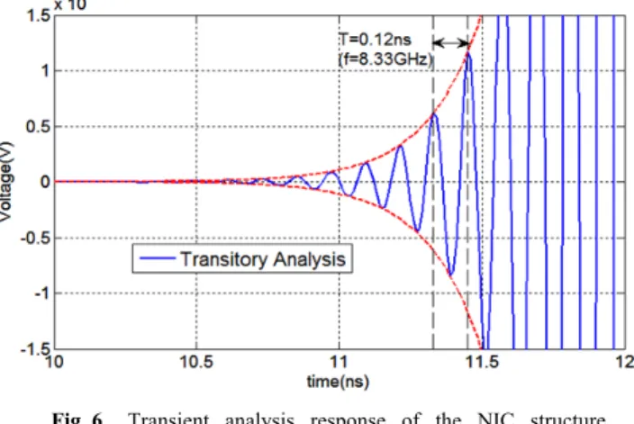
Fig. 6. Transient analysis response of the NIC structure depicted in Fig. 4(a).
12 21 12 21 11 22
1 ( S S S S S S )0 (6)
which equals the denominator of the closed-loop transfer characteristic given in (4). Hence, GL describes the poles of
the closed-loop network. In order to demonstrate the validity of the previous analysis, one of the classic NICs shown in [2] to invert the capacitance C2 in Fig. 4(a), is
passes through the real axis at x = 1.262 corresponding to 1.071 GHz. It can be seen that the GL does not encircle the
+1 point. According to the proposed criterion given through (5), the proposed NIC is stable, agreeing with the loop gain method for the considered load conditions.
In addition to the performed frequency analysis, a time analysis is performed, by means of the AWR® soft-ware, to see the behavior of the NIC with a transient signal (see Fig. 6). These results show that the circuit is clearly unstable and oscillates at 8.33 GHz. In spite of the fact that loop gain method predicted a stable performance, the tran-sient analysis predicts an unstable response. Then, it seems that additional conditions must be added to the previous analysis in order to correctly predict the NIC stability.
3.
Normalized Determinant Function
(NDF)
From the previous analysis, it can be concluded that additional conditions are required for a correct prediction of the NIC stability. In this sense, the so-called normalized determinant function (NDF) ([20] and [21]) can be consid-ered as the only single step method able to predict in a rigo-rous way the stability of any N-port network structure. The NDF was proposed as a method to verify the Rollet proviso conditions in two-port amplifier networks [25].
The goal is, as before, to find out the set of values for ZL and ZS that make the NIC stable. The NDF is defined as
the ratio between the determinant of the network function when all the dependent generators are switched on Δ(s) and the determinant of the network function when all the generators are switched off Δ0(s):
0
( ) ( )
s NDF
s
. (7)
The NDF has some important properties: as the active network behaves as the passive network when ω or σ tends to infinity, the NDF tends to one. The NDF has not any poles in the RHP since Δ0(s) is a passive network and the
denominator of Δ(s) and Δ0(s) are equal. Taking these
properties into account, and using the principle of the argument theorem, it is possible to determine the number of zeroes of the NDF in the RHP (poles of the system in the RHP), as equal to the number of clockwise encirclements, around the origin, that the NDF makes, when it is evaluated from ω = –∞ to ω = ∞. Therefore, the system will be stable if, and only if the NDF does not clockwise encircle the origin of the complex plane.
One of the advantages of the NDF is that it can be easily calculated through the return ratio functions given by Bode. Then the NDF can be given as follows:
0( 1)
k i i
NDF
RR (8)of the network; RR1 is the return ratio of the source i = 1,
when the sources i = 2, 3,…, k are switched on; RR2 is the
return ratio of the source i = 2, when the source i = 1 is switched off, and sources i=3,4,…,k are switched on; and RR3 is the return ratio of the source i = 3, when the sources
i = 1, 2, are off, and sources i = 4, 5,…, k are on. In the same way, RRk is the return ratio of the source i = k, when the sources i = 1, 2,…, k – 1 are switched off. Finally, to calculate each RRi, the dependent source in the trans-con-ductance model, of the ith active element, must be replaced
with the expression –gmVi as it is shown in Fig. 7. Then, evaluating the response of its dependent node to an external excitation V’ of magnitude 1, the RRi can be calculated as:
'
i i
V RR
V
. (9)
In order to use the NDF, or the RR, it is necessary to have a linear model of the transistor or to extract it from the non-linear model or the S-parameters of the device. Fig-ure 7 shows the equivalent circuit of a bipolar transistor without any parasitic elements, all the parasitic elements of the transistor are included in the feed-back network. This circuit allows the access to any internal port, so that the RR can be calculated with the circuit simulator. The NDF can be directly calculated with any circuit simulator and it is able to detect the number of poles of the network function. There must not exist any poles in the RHP for a stable NIC. The main drawback of the NDF is that it requires a prior full linear modeling of each active device around its biasing point, which can be difficult and inaccurate at high frequencies. Other approaches are possible using nonlinear models, but extracting the small signal model and using the NDF is generally the safest one [25].
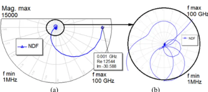
Now, an analysis example is presented to show how the NDF can predict the potential instabilities of NIC cir-cuits. The circuit previously described in Sec. 2.2 will be studied. Figure8 shows the NDF of the circuit, where it can
Fig. 7. Linear equivalent circuit for the bipolar transistor.
(a) (b) Fig. 8. a) NDF of the NIC circuit proposed in Sec. 2.2.
be clearly observed how the NDF encircles the origin in a clockwise sense, so the circuit is unstable as it was previ-ously stated. In addition, the predicted oscillation fre-quency is around 7.45 GHz (the NDF crosses through the negative real axis at that frequency), very close to the one predicted by the transient analysis performed and depicted in Fig. 6. This small discrepancy comes from non-linear effects that modify the original linear RRi functions and, subsequently, the NDF accuracy.
4.
Unified Approach between NDF and
Classic Methods for Stability
Analysis of Non-Foster Forms
It is very useful to work with the impedances or re-flection coefficient during the NICs design. However, it must be pointed out that additional conditions (the proviso) must be defined and satisfied before using any of the meth-ods proposed in Sec. 2. In other words, the classic methmeth-ods can only properly check the stability if the proviso is satis-fied [25–27]. The next subsection shows which are these additional conditions for the methods proposed in Sec. 2, and how they can easily be evaluated using the NDF.
4.1
Additional Conditions for the Reference
Plane Methods
In this section the additional conditions that must be satisfied in order that the reference plane methods studied in Sec. 2.1 are derived to properly predict the stability. Once these additional conditions are fulfilled, the Nyquist analysis of the characteristic equations (Z, Y) can predict the presence of poles in the RHP, and hence the stability of the loaded network.
Firstly, the admittance criterion is used, studying the function YT(ω), where YT(ω) = YNIC(ω) + YL(ω), being YNIC
the admittance provided by the NIC and YL the load
con-nected to the NIC) (see Fig. 1). The analysis in the fre-quency domain of YT(ω) is performed to obtain the Nyquist
plot of YT(ω). The Nyquist criterion provides the number
NZ – NP, where NZ and NP are respectively the number of zeros and poles in the RHP. This number (NZ – NP) corre-sponds with the number of times that the function YT(ω)
encircles the origin of the complex plane when it is evalu-ated from ω = –∞ to ω = ∞.
To be sure that the Nyquist analysis of YT(ω) provides
the number of poles of the system, it is needed that YT(ω)
has not any poles in the RHP. The necessary condition is that YNIC has not any poles in the RHP (visible or hidden
ones). It is very important to point out that the function YNIC
is a reduced function of a bigger network, hence it might not present hidden poles (poles of the system that are not present in YNIC since it is a reduced function), that can
in-validate the Nyquist analysis of YT. On the other hand, YL
will not present any pole in the RHP, because it is a passive network.
The proviso to check before using the admittance criterion is that the YNIC network loaded with short-circuit
has not any poles in the RHP. It is that the NDF does not clockwise encircle the origin ([8] and [25]) (see Fig. 1) as it was explained in Sec. 3.
The additional required conditions when working with the impedance criteria (function ZT(ω)) can be derived
in a similar way: ZNIC must not present any poles in the
RHP when the network is loaded with open-circuit. Once this additionally condition is verified by using the NDF, the Nyquist criteria can be used over ZT to study the stability of
the circuit.
Finally, if the reflection coefficient is used, the addi-tional condition is that ΓNIC has not any poles in the RHP
when the network is loaded with Z0. As in the previous
cases, it can be easily done using the NDF.
4.2
Additional Conditions for the Loop-Gain
Method
In this section the additional conditions for the open-loop methods are derived. These methods include the stability factor K and the methods which use the open-loop gain (see Sec. 2.2).
Firstly, the stability factor methods are used. The ad-ditional condition for the stability factor methods is that the network has not any poles in the RHP when it is loaded with Z0. This analysis can be performed using the NDF
when the circuit is loaded with Z0.
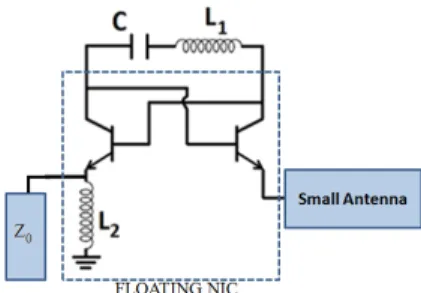
To illustrate this point, the circuit shown in Fig. 9 [4] is studied. The circuit consists on a floating NIC connected between a small antenna and the port Z0 (typically 50 Ω).
In this case the NIC is used to negate the impedance 1/(jωC) + jωL1 in order to compensate the reactance of the
small antenna and hence improve the bandwidth. However, Figure 10 shows that the circuit does not satisfy the suitable proviso, since the NDF encircles the origin when the circuit is loaded with Z0, so the classic stability factor (i.e. Rollet
factor or μ-factor) cannot be used to predict the stability. The second method under study is the one based on the open-loop gain. This method states that the circuit is stable if the denominator of (3) has not any zeroes in the RHP, or, what it is the same, that the function G(ω)·H(ω) does not encircle the –1 point (Nyquist theorem).
(a) (b) Fig. 10. a) NDF of the circuit under study.
b) Zoom around the origin.
However, before using the GLfunction (5) to properly
predict the existence, or not, of poles in the RHP, some additional conditions must be verified:
The first condition states that GL must not have any
poles in the RHP. It does not have any poles if the test function TF = 1 – S11·S22 + S12·S21 –2·S12 has not any
zeroes in the RHP. This can be done by performing the Nyquist analysis of the TF and checking that it does not encircle the origin in a clockwise sense.
The second one is that the numerator of Io/I (4) must
not have any poles (visible or hidden) in the RHP. As in the previous case, it will not have any poles if none of the S parameters have any poles in the RHP and, in addition, the TF has not any zeroes in the RHP (first condition).
In practice, these two aforementioned conditions can be tested as follows. Firstly, the NDF must be calculated over the open-loop network loaded with Z0 to test that S
parameters have not any poles in the RHP. Secondly, the Nyquist analysis over the TF (denominator of GL) must be
undertaken. If both tests are positive, none of them encircle the origin, then GL can be used to predict the existence or
inexistence of poles of the function Io/I.
As an example, it is shown how the circuit presented in Sec. 2.2 (see Fig. 4(a), (b)) does not satisfy the proviso, so the GL function cannot be used to predict the stability.
Figure 11 (a), (b) shows how the first part of the aforemen-tioned proviso conditions is not satisfied (NDF when the network is loaded with Z0) because the NDF does encircle
the origin. Moreover, the second part of the proviso is not fulfilled because the Nyquist analysis of the TF indicates
(a) (b) Fig. 11. a) NDF of the circuit proposed in Sec. 2.2.
b) Zoom around the origin.
Fig. 12. Nyquist analysis of the transfer function TF.
the existence of zeros (poles of the system) in the RHP, as it can be observed in Fig. 12. For this reason, as the proviso is not satisfied, the open-loop gain GL [24] cannot be used
as a predictor of the stability, and it provides incorrect results as it was shown in Sec. 2.2 using the transient analysis (see Fig. 6).
5.
Design Example
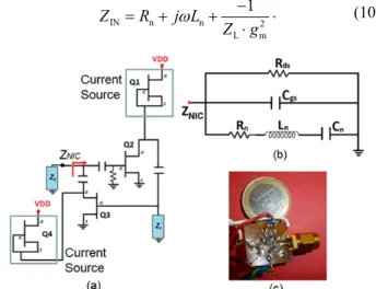
In this section it will be shown how the NDF can be used to predict the stability of a NIC during the linear de-sign step. The NIC is dede-signed to present a negative capac-itor and the chosen topology is the one presented in Fig. 13. It is based on a silicon N-channel dual-gate MOSFET tran-sistor (BF998) with a transconductance gmof25 mS at the
selected bias point (Q2 and Q3 in Fig. 13(a) connected in
a ring topology, and a load ZL to be inverted). Additionally,
two more transistors (Q1 and Q4 in Fig. 13(a)) are used as
currents sources for biasing purpose.
Using a small-signal analysis, the equivalent circuit of the NIC can easily be obtained as it can be seen in Fig. 13(b). Moreover, the effect of RDS and CGS can be
neglected for low frequencies, in such a way that the input impedance can be approximated as (10), where Rn= –1/(g2m·RDS) and Ln= –CGS/g2mare parasitic negative
resistance and negative inductance respectively (being gm
the FET transconductance, CGS the gate-source capacitance
and RDS the drain-source resistor of the FET small signal
model).
IN n n 2
L m
1 Z R j L
Z g
. (10)
As an isolated negative capacitor is always unstable, an additional load ZS is required to make the system stable.
In practice, this load ZS is the one connected to the NIC
inside the application. For instance, if a NIC is used to improve the matching of an electrically small antenna (ESA) the load ZS will be the impedance of the antenna at
the port where it will be connected. The NDF can be used during the design to determine which loads, ZS, make the
circuit stable as it will be shown below. Figure 13(c) shows the prototyped circuit.
The simulations are performed using a real (not loss-less) inductor model of 56 nH (Coilcraft® 0805CS
L = 56 nH, R1 = 13 Ω, R2= 0.34 Ω, C = 0.094 pF,
K = 0.000101√f) and a quality factor of 60. As the induct-ance has a value of 56 nH the expected negative capaci-tance is about Cn= –32 pF, according to (8). Taking this
into account, an analysis of the circuit is performed using the NDF. This analysis shows that the circuit is stable when ZS is a positive capacitor larger, in magnitude, than the
negative one (–32 pF) and it is unstable in any other case:
s n
s n
Stable, Unstable.
C C C C
(11)
To illustrate this behavior, Figure 14 shows the NDF for two values of the Cs capacitor. For Cs = 50 pF the NDF
does not clockwise encircle the origin so the circuit is sta-ble. But in the case of Cs = 25 F the NDF clearly encircles
the origin, so the circuit is unstable. Similar stability crite-ria have been obtained in [28], but the authors consider that the NDF is a more general tool, valid not only for the to-pology of this example but for any other toto-pology. In addi-tion, the use of the NDF also takes into account many ef-fects such as the parasitic efef-fects, the effect of the transmis-sion lines, the biasing networks, the non-idealities of the components, etc. that were not considered in [28].
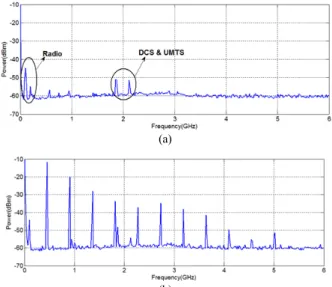
This behavior was also experimented in practice with the manufacturing of a prototype. It can be observed in the measurements obtained with the spectrum analyzer that the behaviors of the manufactured circuits are the expected ones Figure 15(a) corresponds to the stable case of (CS = 50 pF > |Cn|). In this case the circuit is stable since
there is not any signal apart from small peaks correspond-ing to DCS & UMTS and radio interferences. On the other hand, Figure 15(b) shows the spectrum of the unstable case
(a) (b) Fig. 14. a) NDF of the proposed design example.
b) Zoom around the origin.
(a)
(b)
Fig. 15. Spectrum. a) Stable case (CS = 50 pF). b) Unstable case (CS = 25 pF).
(a) (b) Fig. 16. a) NDF of the circuit. b) Zoom around the origin.
(CS= 25 pF < |Cn|). In this case the circuit is clearly
unstable and oscillates at 455 MHz with importance levels in its harmonics.
In addition, the prototype is unstable for CS = 100 pF
and high biasing voltages, which was supposed to be sta-ble. The NDF can also predict this behavior: When the biasing voltage increases, the drain-source voltages of the FETs also do, and therefore the transconductance of the FET can also increase slightly.
Figure 16 shows the NDF of the circuit for two values of the transconductance and it can be observed how when the transconductance increases from 25 mS to 30 mS the circuit turns unstable (the NDF clockwise encircles the origin) as it was observed in the prototype.
(a)
(b)
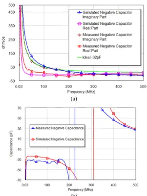
Fig. 17. NIC measurements. a) NIC impedance. b) Equivalent capacitance.
lations are due to the fact that to obtain a negative capacitor depends on the FET transconductance, which is difficult to characterize in practice.
The prototype presented here works up to 200 MHz due to the fact that as a rule of thumb NICs only work up to a frequency ten times smaller than the transient frequency of the transistors [30]. The transistor employed here (BF998) has a transient frequency of 1.9 GHz, so the pro-totype presents the expected bandwidth. A FET transistor has been chosen instead of other with a higher transient frequency because it is easier to obtain accurate linear models at low frequencies to show the validity of the method. At high frequencies, more feedback paths, and more parasitic effects must be considered, so obtaining linear models is more complicated.
However, it is important to remark that although the method has only been validated with a NIC working up to 200 MHz, the method is general and valid no matter the operation frequency as long as accurate linear models of the active devices, passive elements, interconnections are available.
For instance, this NDF method can be used for MMIC where interconnections are not too lossy. Of course this method can also be used for or in Silicon and SiGe pro-cesses where the interconnections are lossy and frequency dependent, including the influence of the layout in the linear model.
For the sake of completeness, the designed and pro-totyped NIC circuit is used as an embedded active match-ing network, for a blade-type small monopole of 22 cm × 25 cm over a FR4 substrate of 1.6 mm in width and εr = 4.3. The intended impedance matching bandwidth
(a) (b)
Fig. 18. Antenna sketch with the embedded NIC. b) NDF of the whole design: antenna+NIC.
(i.e. |S11| < –8 dB) is over a 2 : 1 range (50 ÷ 110 MHz).
Figure 18(a) shows the antenna structure with the embed-ded MN, a vertical slot has been incluembed-ded to force a longer way for the current along the monopole with the purpose of reducing the electrical size of the antenna at the intended frequency range. The same NIC topology, as the one pre-sented in the previous example, is selected for acting as an active MN, but this time with a reactance expected to realize an ideal negative inductor, in order to compensate the capacitive nature of the monopole impedance at lower frequencies. The whole antenna system (antenna+NIC) stability is evaluated by means of the NDF (see Fig. 18(b)), predicting stability.
ZinNIC has to be chosen according to the impedance
needed at the connecting point in the monopole structure, in order to obtain an input impedance (Zinant) as near as
possible to the system impedance (50 Ω). The active matching antenna method, proposed in [29], can be applied in this case, to calculate an analytical impedance (ZMN) to
(a)
(b)
be realized with our NIC circuit. Once the analytical im-pedance ZMN is computed, it is possible to choose a
capac-itor to load the NIC (ZNIC=1/jωC), then a negative inductor,
proportional to the value of the capacitance C, is obtained Ln = –gm2·C. Figure 19(a) shows the computed analytical
ZNIC and the simulated NIC input impedance ZIN.
The new engineered impedance matching band is ob-tained at VHF frequencies, as it is shown in Fig. 19(b) where a fractional impedance bandwidth (FBW) of 63% is obtained. One more advantage of the NDF method stands in the fact that it is possible to include the antenna S-pa-rameter model in the stability analysis.
6.
Conclusion
This paper proposes the use of the Normalized De-terminant Function (NDF) as a tool to analyze the stability of NIC circuits (or any circuit in general). The NDF can easily take into account different effects such as the para-sitic effects, the non-idealities, the effect of the biasing networks, the effect of the transmission lines, etc. It has been shown that classic stability methods such as reference plane, stability factor (K or μ) or open-loop gain methods can yield to incorrect results. All the classic methods work with parameters extracted from reduced networks, so some poles of the complete networks could be missed and then they cannot be detected. For these reasons, these methods cannot be considered by themselves as universal methods for the stability analysis. However, if some additional con-ditions were satisfied, the so called proviso concon-ditions, all these methods can still work properly. All these necessary additional conditions are based in the NDF. Nevertheless, the authors conclude that the analysis based on the NDF always yields correct predictions regarding the stability and the oscillation frequency and, hence, it is the safer and quicker option for the designers. On the other hand, the main drawback of the NDF for the NIC design is that the accurate linear models of the active devices are required.
Finally, the proposed NDF method has been used to successfully design a negative capacitor working up to 200 MHz. It has been shown how the NDF predicts the loads and the biasing conditions that make the circuits stable or unstable and how these predictions are in perfect agreement with the performed measurements.
References
[1] SUSSMAN-FORT, S.E., RUDISH, R.M. Non-foster impedance matching of electrically-small antennas. IEEE Transactions on Antennas and Propagation. 2009, vol. 57, no. 8, p. 2230–2241. ISSN 0018-926X, 1558-2221. DOI:10.1109/TAP.2009.2024494 [2] SUSSMAN-FORT, S.E., RUDISH, R.M. Non-foster impedance
matching for transmit applications. In IEEE International Workshop on Antenna Technology Small Antennas and Novel Metamaterials. New York (USA), March 2006, p. 53–56. DOI: 10.1109/IWAT.2006.1608973
[3] SUSSMAN-FORT, S.E. Non-Foster vs. active matching of an electrically-small receive antenna. In 2010 IEEE Antennas and
Propagation Society International Symposium. Toronto (ON, Canada), 2010, p. 1–4. DOI: 10.1109/APS.2010.5562052
[4] ABERLE, J.T. Two-port representation of an antenna with application to non-foster matching networks. IEEE Transactions on Antennas and Propagation. 2008, vol. 56, no. 5, p. 1218–1222. ISSN 0018-926X. DOI: 10.1109/TAP.2008.922173
[5] SUÁREZ, A., QUÉRÉ, R. Stability Analysis of Nonlinear Micro-wave Circuits. Artech House, 2003. ISBN 978-1-58053-586-1. [6] BROWNLIE, J.D. On the stability properties of a negative
impedance converter. IEEE Transactions on Circuit Theory. 1966, vol. 13, no. 1, p. 98–99. ISSN 0018-9324. DOI: 10.1109/TCT.1966.1082542
[7] HOSKINS, R. F. Stability of negative-impedance convertors.
Electronics Letters. 1966, vol. 2, no. 9, p. 341–341. ISSN 1350-911X. DOI: 10.1049/el:19660287
[8] BROWNLIE, J. D. Small-signal responses realizable from d.c.-biased devices. Proceedings of the Institution of Electrical Engineers. 1963, vol. 110, no. 5, p. 823–829. ISSN 0020-3270. DOI: 10.1049/piee.1963.0111
[9] STERN, A. P. Stability and power gain of tuned transistor amplifi-ers. Proceedings of the IRE, 1957, vol. 45, no. 3, p. 335–343. ISSN 0096-8390. DOI: 10.1109/JRPROC.1957.278369
[10] DAVIES, A. Stability properties of a negative immittance con-verter. IEEE Transactions on Circuit Theory, 1968, vol. 15, no. 1, p. 80–81. ISSN 0018-9324. DOI: 10.1109/TCT.1968.1082775 [11] MIDDLEBROOK, R.D. Measurement of loop gain in feedback
systems. International Journal of Electronics Theoretical and Experimental. 1975, vol. 38, no. 4, p. 485–512. ISSN 0020-7217. DOI: 10.1080/00207217508920421
[12] VENDELIN, G., PAVIO, A.M., ROHDE, U.L. Microwave Circuit Design using Linear and Nonlinear Techniques. 2nd ed.New York: John Wiley & Sons, 1990 [accessed 24th May, 2016]. ISBN 978-0-471-41479-7.
[13] JACKSON, R.W. Rollett proviso in the stability of linear microwave circuits-a tutorial. IEEE Transactions on Microwave Theory and Techniques, 2006, vol. 54, no. 3, p. 993–1000. ISSN 0018-9480. DOI: 10.1109/TMTT.2006.869719
[14] BODE, H. W. Network Analysis, Feedback Amplifier Design. New York, USA: Van Nostrand, 1945.
[15] ROLLETT, J. Stability and power-gain invariants of linear two-ports. IRE Transactions on Circuit Theory, 1962, vol. 9, no. 1, p. 29–32. ISSN 0096-2007. DOI: 10.1109/TCT.1962.1086854 [16] EDWARDS, M. L., SINSKY, J.H. A new criterion for linear
2-port stability using a single geometrically derived parameter. IEEE Transactions on Microwave Theory and Techniques, 1992, vol. 40, no. 12, p. 2303–2311. ISSN 0018-9480. DOI: 10.1109/22.179894 [17] EDWARDS, M. L., CHENG, S., SINSKY, J.H. A deterministic
approach for designing conditionally stable amplifiers. IEEE Transactions on Microwave Theory and Techniques, 1995, vol. 43, no. 7, p. 1567–1575. ISSN 0018-9480. DOI: 10.1109/22.392916 [18] KUROKAWA, K. Some basic characteristics of broadband
negative resistance oscillator circuits. The Bell System Technical Journal, 1969, vol. 48, no. 6, p. 1937–1955. ISSN 0005-8580. DOI: 10.1002/j.1538-7305.1969.tb01158.x
[19] UGARTE-MUNOZ, E., HRABAR, S., SEGOVIA-VARGAS, D., et al. Stability of non-foster reactive elements for use in active metamaterials and antennas. IEEE Transactions on Antennas and Propagation, 2012, vol. 60, no. 7, p. 3490–3494. ISSN 0018-926X. DOI: 10.1109/TAP.2012.2196957
ports. In The IEEE 3rd International Workshop on Integrated
Nonlinear Microwave and Millimeterwave Circuits. Duisburg (Germany), 1994, p. 93–107. DOI: 10.1109/INMMC.1994.512515 [22] OHTOMO, M. Stability analysis and numerical simulation of
multidevice amplifiers. IEEE Transactions on Microwave Theory and Techniques, 1993, vol. 41, no. 6, p. 983–991. ISSN 0018-9480. DOI: 10.1109/22.238513
[23] NYQUIST, H. Regeneration theory. The Bell System Technical Journal, 1932, vol. 11, no. 1, p. 126–147. ISSN 0005-8580. DOI: 10.1002/j.1538-7305.1932.tb02344.x
[24] RANDALL, M., HOCK, T. General oscillator characterization using linear open-loop S-parameters. IEEE Transactions on Microwave Theory and Techniques, 2001, vol. 49, no. 6, p. 1094–1100. ISSN 0018-9480. DOI: 10.1109/22.925496
[25] JACKSON, R.W. Criteria for the onset of oscillation in microwave circuits. IEEE Transactions on Microwave Theory and Techniques, 1992, vol. 40, no. 3, p. 566–569. ISSN 0018-9480. DOI: 10.1109/22.121734
[26] STEARNS, S.D. Incorrect stability criteria for non-foster circuits. In Proceedings of IEEE 2012 International Symposium on Antennas and Propagation. Chicago (IL, USA), 2012, p. 1–2. DOI: 10.1109/APS.2012.6348832
[27] GONZALEZ-POSADAS, V., SEGOVIA-VARGAS, D., JIMÉ-NEZ, J.L., et al. Study of the stability properties of negative impedance converters using the gain-loop method. In IEEE Antennas and Propagation Society International Symposium (APSURSI). Washington (USA), 2011.
[28] KOLEV, S., DELACRESSONNIERE, B., GAUTIER, J.-L. Using a negative capacitance to increase the tuning range of a varactor diode in MMIC technology. IEEE Transactions on Microwave Theory and Techniques, 2001, vol. 49, no. 12, p. 2425–2430. DOI: 10.1109/22.971631
[29] ALBARRACIN-VARGAS, F. Sensitivity analysis for active matched antennas with non-foster elements. IEEE Transactions on Antennas and Propagation, 2014, vol. 62, no. 12, p. 6040–6048. ISSN 0018-926X. DOI: 10.1109/TAP.2014.2364811
[30] HRABAR, S., KROIS, I., KIRICENKO, A. Towards active dispersion-less ENZ metamaterial for cloaking applications.
Metamaterials, 2010, vol. 4, no. 2-3, p. 89–97. ISSN 1873-1988. DOI: 10.1016/j.metmat.2010.07.001
About the Authors ...
Daniel SEGOVIA-VARGAS (M’98) was born in Madrid,
Spain, in 1968. He received the telecommunications engi-neering and the Ph.D. degrees from the Polytechnic Uni-versity of Madrid, Madrid, in 1993 and 1998, respectively. From 1993 to 1998, he was an Assistant Professor at Valladolid University, Valladolid. Since 1998, he has been an Associate Professor at Carlos III University, Madrid, where he is in charge of the microwaves and antenna courses. He has authored and coauthored more than 80 technical conference, letters, and journal papers. His re-search areas are printed antennas, active radiators and arrays, smart antennas, LH metamaterials, and passive circuits. He has also been member of the European Projects Cost260, Cost284, and COST IC0603.
José Luis JIMÉNEZ-MARTÍN was born in Madrid,
Spain, in 1967. He received the B.S. degree in Electrical
neering, and the Ph.D. degree from the Universidad Politéc-nica de Madrid (UPM), Madrid, in 1991, 2000, and 2005, respectively, and the master’s degree in high strategic studies from CESEDEN (organization pertaining to the Spanish Ministry of Defense), Madrid, in 2007. He is cur-rently an Associate Professor with UPM. He has authored or co-authored over 60 technical conference, letters, and journal papers. His current research interests include oscil-lators, amplifiers, and microwave technology.
Ángel PARRA-CERRADA was born in Madrid, Spain,
in 1975. He received the B.S. and M.S. degrees in Electri-cal Engineering from the UPM, Madrid, in 1997 and 2003, respectively. He has been a Lecturer in Signal The-ory and Communications with UPM since 2008. He is involved in the private sector in aeronautical and naval projects. His work is focused on electromagnetic interfer-ence and compatibility. His current research interests in-clude secondary radio detection and ranging, active anten-nas, oscillators, microstrip antenanten-nas, composite right/left handed lines and metamaterials, microwave technology, and lightning protection.
Fernando ALBARRACIN-VARGAS was born in
Bo-gotá, Colombia in 1985. He received the Engineer degree in Electronics from National University of Colombia, in 2008 and the Master in Multimedia and Communications from the Carlos III University in Madrid, Spain, in 2014. From 2010 to 2011, he was a Research Assistant with the International Centre for Physics in the Univesidad Nacional de Colombia, Bogotá, Colombia. He is currently working towards the Ph.D. degree with the Group of Radiofre-quency, Electromagnetism, Microwaves and Antennas (GREMA) at the Carlos III University in Madrid. His pre-sent research interests include metamaterials based struc-tures, non-Foster elements, ultra-wideband antennas, ac-tive-matching and miniaturization of antennas.
Eduardo UGARTE-MUÑOZ was born in Caracas,
Vene-zuela in 1983. He received the Engineer degree in Tele-communications from the Carlos III University in Madrid, Spain, in 2008 and the Master in Multimedia and Commu-nications in 2011. His research interests are metamaterials, active antennas, RFID systems, array antennas, metasur-faces, CMOS, non-Foster elements and active matching.
Vicente GONZALEZ-POSADAS was born in Madrid