Analysis and 2D Simulation of a Hexapod Robot Leg for Remote Exploration
J. Torres 1, G. Romero 2, J. Felez 2, J. Gomez-Elvira 1
1 Centre for Astrobiology INTA/CSIC,
Ctra de Torrejón a Ajalvir, km 4. 28850 Torrejón de Ardoz, Madrid. (Spain) E-mail: [email protected], [email protected]
2
ETS Industrial Engineering, Technical Univ. of Madrid UPM C/Jose Gutierrez Abascal, 2.
28006 Madrid. (Spain)
E-mail: [email protected], [email protected]
Abstract—. A walking machine is a wheeled rover alternative, well suited for work in an unstructured environment and specially in abrupt terrain. They have some drawback like speed and power consumption, but they can achieve complex movements and protrude very little the environment they are working on. The locomotion system is determined by the terrain conditions and, in our case, this legged design has been chosen based in a working area like Rio Tinto in the South of Spain, which is a river area with abrupt terrain. A walking robot with so many degrees of freedom can be a challenge when dealing with the analysis and simulations of the legs. This paper shows how to deal with the kinematical analysis of the equations of a hexapod robot based on a design developed by the Center of Astrobiology INTA-CSIC following the classical formulation of equations.
Keywords- Hexapod robot, walking machines, rover, remote exploration, simulation.
I. INTRODUCTION
When faced with the task of designing a rover [1, 2], the operation area where the robot is going to explore is an important requirement for the type of design chosen. For abrupt terrains, like Rio Tinto a walking robot design looks like a good option as it can adapt better to rocky and wet areas that were chosen by the scientist as the best area of interest for analysis, also another requirement for the rover was to perform slow and precise movements. The Center of Astrobiology scientists needed the area to be protruded as less as possible, for this reason a walking rover was chosen as they are less harmful to the environment and can perform precise movements. Other options like rover wheels can damage the terrain the scientists want to analyze [3]. On the contrary as wheeled rovers, walking robots present various handicaps like high design complexity and large power consumption due to the amount of actuators needed; another very important problem the engineer has to face is dealing with the kinematic analysis of the trajectory equations.
The aim of this paper is to introduce the first analysis approach in order to obtain the necessary equations of a six legged robot in an easy and robust way.
II. ROBOT DESIGN
The design [4] corresponds to a hexapod, and has three independent DC motor actuator in each leg, with a walking motion that can be performed as follows: the robot can stand in three legs in a triangular configuration meanwhile the other three legs are in the air. To obtain the normal translation movement, the three legs on the floor can perform a rowing motion forward and when they reached the maximum motion, the legs in the air can come down and the same procedure will follow. With these movements we can avoid having the 18 actuators acting at the same time.
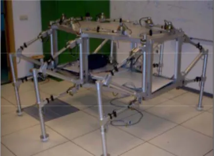
As it can be seen in the next figure, each of the legs has three independent degrees of freedom, being two of them controlled by linear actuators and the other by a DC gear motor.
Figure 1. Composition of the prototype design.
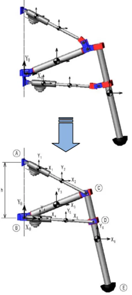
Below is a detailed sketch of the leg and the movement of all the actuators involved. The maximum angles and positions that it can move will depend on the actuators elongation, collisions, large force or moments acting and unstable positions.
III. MATHEMATICAL MODELLING OF ONE LEG If we look at figure 3 below we have summarized the movement elements of one of the legs. All legs are independent but they all perform the same motions and have the same degrees of freedom if we obtain the equations for one leg, we will have the kinematic equations of the rest.
Figure 3. Sketch of the simplified hexapod leg.
When faced with a complex 3D problem as the one we are analyzing you need to first simplify the problem by determining the degrees of freedom and restriction that you have. An important point is to always take the same positive and negative criteria for the moments and translations. For this paper we will not introduce the rowing motion of the leg, it will be based in two degrees of freedom; the third movement will be dealt in a future paper.
Considering as restrictions the reference position the system X0,Y0, we can begin the setting of equations.
To obtain the different kinematic equations, we need to consider initially three points (A, B and C) in which rotational movement exists due to the elongation and contraction of the DC actuators.
Writing the necessary information in matrix form and choosing a system of reference parallel to the world system of reference, but moving it with the center of gravity of each bar, we can write the equations as:
» ¼ º « ¬ ª » » ¼ º « « ¬ ª » ¼ º «
¬ ª » ¼ º « ¬ ª
h L
y
x 0
0 2 sin
cos cos
sin 1
1 1
1 1 1
1
I I
I
I (1)
Finally, obtaining the equations from the above system, we would have the equations that define the behavior law of the point A:
0 sin
2 1
1 1 I
L
x (2)
0 cos
2 1
1
1 h
L
y I (3)
Applying the same concept to the rest, we would have the behavior law of points B and C:
0 sin
2 3
3
3 I
L
x (4)
0 cos
2 3
3
3 I
L
y (5)
0 sin
2 4
4
4 I
L
x (6)
0 cos
2 4
4
4 I
L
y (7)
0 sin 2 sin
2 2 3 3 3
2
2 I I
L x L
x (8)
0 cos 2 cos
2 2 3 3 3
2
2 I I
L y L
y (9)
0 sin 2 sin
2 2 6 6 6
2
2 I I
L x L
x (10)
0 cos 2 cos
2 2 6 6 6
2
2 I I
L y L
y (11)
In previous equations, it has been taken into account that in point B, point which goes linked to main body of the hexapod robot and reference system of the leg, converge bars 3 and 4, while bars 2, 3 and 5 converge in point C.
The DC actuators, they let only a relative X movement between both extremes, being the same angle over bodies 1 and 2:
0
2 1I
I (12)
In addition to the DC actuator, the necessity of being co-axial both bars, it´s necessary satisfy that a virtual vector from one to the other must be in the same direction that their directions (I1=I2), which is corresponding with a vector product equal to zero. If we write in matrix form the previous equation as a difference of the positions linked to the extremes:
0 sin cos
1 1 1 2
1 2
» ¼ º « ¬ ª u » ¼ º « ¬ ª
I I
y y
x x
Doing it, the necessary equation to define the relative movement between bodies 1 and 2 is the next:
x2x1sinI1y2y1cosI1 0 (14)In a similar way, for the actuator which actuates over bodies 4 and 5, the defining equation would be:
0
5 4I
I (15)
x5x4sinI4y5y4cosI4 0 (16)Finally, point D goes over body 6, which means that a virtual vector between the reference system of body 6 and point D5 must be parallel to the vector associated with the
direction of body 6.
0 sin cos cos 2 sin 2 6 6 6 5 5 5 6 5 5 5 » ¼ º « ¬ ª u » » » ¼ º « « « ¬ ª ¸¹ · ¨© § ¸¹ · ¨© § I I I I y L y x L x (17)
Doing it, we would have the equation that defines the behavior law of the point D:
0 cos cos 2 sin sin
2 5 6 6 5 5 5 6 6
5
5 ¸
¹ · ¨ © § ¸¹ · ¨© § ¸ ¹ · ¨ © § ¸¹ · ¨©
§ I I L I y I
y x
L
x (18)
Once the 15 cinematic equations have been found, it is necessary to write the dynamic equations by deriving it from the Jacobean matrix.
> @ ... ... ... ... ... ... ... ... ... ... ... ... ... 0 ... 0 0 0 0 0 ... 0 sin 2 1 0 0 ... 0 cos 2 0 1 ... 3 1 2 1 1 1 2 1 1 1 m n n m L L x y x J M M I M I M I I w w w w w w w w w w u (19)
Finally considering the reactions in each point [5] in which we are considering each equation, and external forces as gravity, momentums due to the ground reaction, actuator forces, etc…, we could write in matrix form the dynamic equations to do the necessary simulations.
> @ » » » » » » ¼ º « « « « « « ¬ ª » » » » » » ¼ º « « « « « « ¬ ª » » » » » » ¼ º « « « « « « ¬ ª » » » » » » ¼ º « « « « « « ¬ ª A u n D B A A T n m n n M M F F R R R R J y x J J m m Y X X Y X ... ... ... ... 1 1 1 1 1 1 1 1 1 I I (20)
IV. 2DHEXAPOD ROBOT
To verify that the system of equations here presented is working correctly, the easiest way is to check the resulting position of the coordinates shown in Figure 3 for one leg in different times. Shown below, the resolution of this equations for segments 1, 2, 3 and for a time interval of 0.1s, taking gravity and proportional lengths and masses.
TABLE I.RESOLUTION OF EQUATIONS FOR T=0-0.1 S
t 0.00 0.05 0.10
x1 0.2165 0.2146 0.2147
y1 0.1250 0.1283 0.1280
I1 1.0472 1.0321 1.0332
x2 0.1083 0.1148 0.1143
y2 0.0625 0.0686 0.0879
I2 1.0472 1,0321 0.9890
x3 0.2165 0.2193 0.2272
y3 -0.1250 -0.1201 -0.1042
I3 1.0472 1.0699 1.1409
… … … …
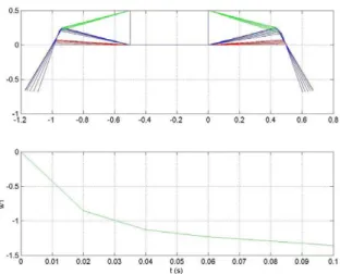
This position and angles of our leg segments are needed to verify that our relations between equations were performed in the correct way. This can be checked by trigonometry relations with the table shown above or it is easy to check by representing these values in a plot. To show a more realistic robot, the real dimensions of the box that carries the instrument has been added (fixed) and a second symmetrical leg is shown [6]. Both have been set with the same scheme. The angular velocity is shown for the right leg
Z1. This represents the movement of both legs with only
mass and gravity acting for 0.1 seconds.
Figure 4. Movement due to mass and gravity
The equations described previously let us easily input and simulate forces in the actuators, obtaining the position, velocity and acceleration of the leg. In figure 5 a force of 50N in actuator 1 is making the legs fall not freely. The same type of graph as the one used for the verification of the equations is shown. The angular velocity in body 1 change compared to the previous graph which was free fall due to mass and gravity.
Figure 5. Movement due to 50N load in actuator 1.
When working with the six legs of the real hexapod, these movements shall be studied carefully as can lead to high forces on the structure that can lead to a deformations or malfunction of one of the actuators. To do it in our 2D model, it´s necessary to obtain the equations not for only one leg, but for both legs linked to the instrument box, in which will be allocated the reference system.
Figure 6. Sketch of the two legs and box instrument composition.
In the previous figure, one of the differences with the model presented in figure 3 is that the connection points of both legs are belonging to the box instrument, transmitting reactions between all the implied elements. In addition, such as it´s possible to see in fig. 6 the lower points of both legs, which are in contact (in figure) with the ground, have a vertical and horizontal restrictions to be immobile. Applying these restrictions, the box and the others bodies will obtain their final positions taking into account the forces of each actuator.
To write the necessary equations corresponding with the different variables (X), we need to consider the same way to get eq. (20), obtaining it in matrix form and considering reactions () and external forces (3):
>
@
>
@
>
@
> @
>
@
> @
>
> @
>
@
> @
@ >
>
>
@
@
@
>
@
>
@
>
@
»
»
»
¼
º
«
«
«
¬
ª
»
»
»
¼
º
«
«
«
¬
ª
»
»
»
¼
º
«
«
«
¬
ª
»
»
»
¼
º
«
«
«
¬
ª
2 1
2 1 2
1 2
1
2 1
LEG BOX LEG
LEG BOX LEG T
LEG BOX
LEG
LEG BOX LEG
LEG BOX
LEG
J
J
J
M
M
M
X
X
X
(21)
A previous study done by the authors [7] in a static sub case of the robot with a configuration of high acting forces, it shows a maximum force of 1200 N over actuator 1 in the worst case, being necessary to design its section area to withstand the forces acting [8]. By using previous equations, a 50N force has been applied to the upper actuator in the right leg. For an easier interpretation, in the figure below the actuators have not been represented.
Figure 7. Secuence of real movement of the instrument box
In the above figure, it´s possible see how a reduction of the length of the actuator means a movement of the box instrument. If the actuator force had been done over left and
right actuators at same time, it would create the rise or the fall of the box, doing this combination when it is necessary.
Figure 8. Validation of the movement of the instrument box
The obtained values have been verified [9] in order to check all the motions obtained from the simulation for the step interval 0-0.1seconds:
TABLE2.VALIDATION OF EQUATIONS (18) FOR T=0-0.1 SECONDS
t simulation 3D
I3 53.03º 52.89º
In figure 6 was possible to look the common configuration used to obtain the movement of the box instruments; nevertheless, if we consider some configurations (e.g. fixed length in upper actuators, and lower actuators working at same way), we need to permit horizontal movement of the contact points. In those cases, the mathematical algorithm used to found the solution of the equations system will not converge and it´s necessary to eliminate the horizontal restriction of the contact point in which exist less horizontal reaction due to will be this point, and not the other one, the extreme to move and readapt.
Figure 9. Vertical reactions over contact points.
Other easily way to find the horizontal reaction in each point is analyzing the vertical reactions in each point necessary to obtain the equilibrium (fig. 9); the horizontal reactions will be proportional to the vertical by using the coefficient adherence ‘P’.
Once the new horizontal coordinates has been found, the movement analysis will continue fixing the two extreme points again.
Figure 10. Movement due to 50N load in rigth upper actuators.
Now that the equations have been verified it´s possible to start working with the equations of the six legs [10]. This will be very simulation time consuming as each leg will have
its independent set of equations. When the six legs are combined together care has to be taken in were you take the common origin of coordinates for all the legs. This paper deals with two degrees of freedom in each leg but care will have to be taken with the rowing motion in further work. Next figure shows the final aspect of use 6 legs, in which have been represented the same movement that figure 7 for all three right upper actuators.
V. RESISTANCE FORCES
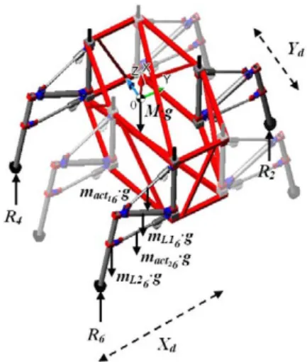
One time our system of equations has been written, the resistance forces can be found. These are very important values as it will help to estimate and dimension the size the actuators that the hexapod will need, also very important information values to validate the maximum stresses and strains that can act on the structure which has to be designed to support all the weights of the instruments on board for all the different configurations of the legs. The reactions are found in the worst case assuming that the hexapod is standing in three legs. The other three legs do not have a ground load reaction but contribute with their weight and displacement configuration (fig. 9).
The figure shown below shows the ground reaction of Leg 1 for some of the worst configuration that the six legs will achieve.
Figure 11. X distance of Leg1 vs. Reaction
Figure 12. Static model reaction results
Figure 11 shows how the reaction with the ground value on Leg1 changes with the distance. To validate our method
VI. CONCLUSIONS.
After setting the system of equations for each leg, it has been validated mathematically and geometrically by trigonometry rules. These equations envolve very large matrices that can lead to common mistakes and care should be taken in this step to verify the performance of the equations. From the degrees of freedom of each leg we have analyzed a two leg system and the complete case adding the box instrument.
Finally and shortly has been calculated the reactions for the worst case configuration: The information from the reactions are necessary to the final design, providing the information to dimension the actuators which will be the heart of the system. It will all give important information about how the structure will suffer and how robust it will have to be.
VII. FUTURE WORK
In the presented paper, we have studied a 2D model and we have taken only two actuators per leg. The third actuator that controls the rowing motion that allows advancing in the trajectory has to be added. This will enable to simulate trajectories that will let the scientists and engineers learn the behavior that the robot will have before testing the commands on the real robot. This will be the work task to be performed in the following months and will be dealt in future articles.
In order to create a more realistic model, resistance forces should be added to the equations to simulate friction and slow the system for a more realistic behavior.
REFERENCES
[1] Song, S. M., Waldron, K. J. 1989 . “Machines that walk”. MIT press. [2] Torres, F., Pomares, J. 2002. “Robots y Sistemas Sensoriales”.
Prentice Hall.
[3] Barrientos, A., Peñin, L. F. 1997. “Fundamentos de Robótica”. McGraw-Hill.
[4] Waldron, K. J., Vohnout, V. J., Pery, A., McGhee, R. B. 1984. “Configuration design of the adaptive suspension vehicle”. International Journal of Robotics Research, Vol. 3, Nº2, pp37-48. [5] Beer,Johnston,Cornwell,2009.“Vector Mechanics for Engineers:
Dynamics”. McGraw-Hill Science.5th Edition
[6] Chapra,2006” Appied numerical models with matlab” McGraw-Hill Science.2nd Edition.
[7] Torres, J., Romero, G., Gómez-Elvira, J., Maroto., J. 2008. “Analysis and Simulation of the Leg of an Hexapod Robot for Remote Exploration“. European Simulation Multiconference 2008, pp 28-34. [8] Gere, J. M., Timoshenko, S. P. 1990. “Mechanics of materials”. PWS
publishing Company. 3rd Edition.
[9] Song, S.M., Waldron, K.J., Kinzel, G.L. 1985. “Computer-aided geometric design of legs for a walking vehicle”. Mechanism and Machine theory, Vol. 20, Nº6, pp 587-596.