Empirical basis for the development of adaptative interfaces : behavioral and neurophysiological evidences of decision making and expertise development in a sequencial choice scenario

Texto completo

(1)PONTIFICIA UNIVERSIDAD CATÓLICA DE CHILE SCHOOL OF ENGINEERING. EMPIRICAL BASIS FOR THE DEVELOPMENT OF ADAPTATIVE INTERFACES: BEHAVIORAL AND NEUROPHYSIOLOGICAL EVIDENCES OF DECISIONMAKING AND EXPERTISE DEVELOPMENT IN A SEQUENCIAL CHOICE SCENARIO. CRISTÓBAL MATÍAS MOENNE VARGAS. Thesis submitted to the Office of Graduate Studies in partial fulfillment of the requirements for the degree of Doctor in Engineering Sciences Advisors: DOMINGO MERY DIEGO COSMELLI. Santiago de Chile, October 2017. Ó 2017, Cristóbal Matías Moenne Vargas.

(2) PONTIFICIA UNIVERSIDAD CATÓLICA DE CHILE SCHOOL OF ENGINEERING. EMPIRICAL BASIS FOR THE DEVELOPMENT OF ADAPTATIVE INTERFACES: BEHAVIORAL AND NEUROPHYSIOLOGICAL EVIDENCES OF DECISIONMAKING AND EXPERTISE DEVELOPMENT IN A SEQUENCIAL CHOICE SCENARIO. CRISTÓBAL MATÍAS MOENNE VARGAS. Members of the Commitee: DOMINGO MERY DIEGO COSMELLI VLADIMIR LÓPEZ CRISTIÁN TEJOS MAX CHACÓN JEAN-PHILIPPE LACHAUX JORGE VÁSQUEZ. Thesis submitted to the Office of Graduate Studies in partial fulfillment of the requirements for the Degree of Doctor in Engineering Sciences. JORGE VÁSQUE Santiago de Chile, October 2017. Ó 2017, Cristóbal Matías Moenne Vargas.

(3) Gratefully to my family and friends. ii.

(4) ACKNOWLEDGEMENTS. Foremost, I would like to express my sincere gratitude to my advisors Professor Diego Cosmelli and Professor Domingo Mery for allowing me to make possible my Ph.D study and research: thanks for your thoughtful guidance. Also, I want to thank my Thesis Committee for all their helpful suggestions and time. I offer my sincere appreciation for the learning opportunities provided by my committee. I am deeply grateful to Professor Vladimir López for helpful discussions and excellent comments, but also for listening to me on any occasion. I would like to thank my fellow labmates: Rodrigo Vergara, Constanza Baquedano, Gonzalo Boncompte, and Catherine Andreu for being always around: thanks for all the chitchatting and procrastination time we spend together. Specially, I am grateful to Rodrigo Vergara for being a friend and partner throughout all this process. Most importantly, none of this would have been possible without the love and patience of my family: my grandparents René Moenne and Melita Geister, my parents Juan Carlos Moenne and Silvia Vargas, my aunt Edith Moenne, and my sister Isabel Moenne and her husband Fabián Sepúlveda. Thank you for their faith in me and for supporting me spiritually throughout my studies. Last but not least, to my caring, loving and supportive soul mate, Cristina Jara: my deepest gratitude, my heartfelt thanks.. This work was supported by the Chilean National Council of Scientific and Technological Research (CONICYT) National PhD grant number 21110823. iii.

(5) TABLE OF CONTENTS. ACKNOWLEDGEMENTS. iii. LIST OF TABLES. vi. LIST OF FIGURES. vii. LIST OF SYMBOLS. x. ABSTRACT. xiii. RESUMEN. xv. 1.. 2.. Outline. 1. 1.1.. Motivation . . . . . . . . . . . . . . . . . . . . . . . . . . . . . . . . .. 1. 1.2.. Approach . . . . . . . . . . . . . . . . . . . . . . . . . . . . . . . . . .. 2. Introduction 2.1.. Electrophysiology. 4 . . . . . . . . . . . . . . . . . . . . . . . . . . . . .. 9. 3.. Hypothesis. 13. 4.. Objectives. 14. 5.. Methods. 15. 5.1.. Task . . . . . . . . . . . . . . . . . . . . . . . . . . . . . . . . . . . . .. 15. 5.2.. Participants . . . . . . . . . . . . . . . . . . . . . . . . . . . . . . . . .. 18. 5.3.. Modeling Framework . . . . . . . . . . . . . . . . . . . . . . . . . . . .. 19. 5.3.1.. Low-level Actions vs Strategies . . . . . . . . . . . . . . . . . . . .. 19. 5.3.2.. Behavioral Modeling . . . . . . . . . . . . . . . . . . . . . . . . . .. 24. 5.3.3.. Scores . . . . . . . . . . . . . . . . . . . . . . . . . . . . . . . . .. 31. 5.3.4.. Clustering . . . . . . . . . . . . . . . . . . . . . . . . . . . . . . .. 32. Recordings . . . . . . . . . . . . . . . . . . . . . . . . . . . . . . . . .. 33. 5.4.. 5.4.1.. Mouse-Tracking Recordings . . . . . . . . . . . . . . . . . . . . . . iv. 33.

(6) 5.4.2. 6.. 7.. 8.. Electrophysiological Recordings . . . . . . . . . . . . . . . . . . . .. Results. 35 39. 6.1.. Behavioral Results . . . . . . . . . . . . . . . . . . . . . . . . . . . . .. 40. 6.2.. Model Parameter Dependence . . . . . . . . . . . . . . . . . . . . . . .. 40. 6.3.. Individual Differences . . . . . . . . . . . . . . . . . . . . . . . . . . .. 42. 6.4.. Predicting Participants’ Choices . . . . . . . . . . . . . . . . . . . . . .. 46. 6.5.. Mouse-Tracking . . . . . . . . . . . . . . . . . . . . . . . . . . . . . .. 50. 6.6.. Electrophysiological Results . . . . . . . . . . . . . . . . . . . . . . . .. 53. 6.6.1.. Checkerboard Probes . . . . . . . . . . . . . . . . . . . . . . . . . .. 53. 6.6.2.. Binary Choice ERP Components . . . . . . . . . . . . . . . . . . . .. 56. 6.6.3.. Feedback ERP Components . . . . . . . . . . . . . . . . . . . . . .. 65. Discussion. 69. 7.1.. Modeling Framework . . . . . . . . . . . . . . . . . . . . . . . . . . . .. 69. 7.2.. Task Structure. . . . . . . . . . . . . . . . . . . . . . . . . . . . . . . .. 72. 7.3.. Temporal and Spatial Encoding Criteria . . . . . . . . . . . . . . . . . .. 73. 7.4.. Electrophysiological Analysis . . . . . . . . . . . . . . . . . . . . . . .. 75. 7.5.. Individual Differences among Users . . . . . . . . . . . . . . . . . . . .. 76. Conclusions and Future Outlook. 78. References. 79. v.

(7) LIST OF TABLES. 5.1. Icon-concept mapping . . . . . . . . . . . . . . . . . . . . . . . . . . . . .. 17. 5.2. Formal definitions of the strategies . . . . . . . . . . . . . . . . . . . . . .. 22. 6.1. Statistics for mouse movements clustered by the most likely observation predicted by the behavioral modeling . . . . . . . . . . . . . . . . . . . . .. 50. 6.2. Statistics for mouse movements clustered by behavioral modeling prediction .. 52. 6.3. Summary of significant spatiotemporal statistics for binary choice EEG signals. 6.4. separated by observation prediction . . . . . . . . . . . . . . . . . . . . . .. 58. Summary of significant spatiotemporal statistics for feedback EEG signals . .. 66. vi.

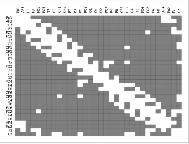
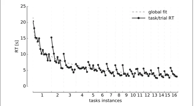
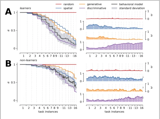
(8) LIST OF FIGURES. 5.1. Schematic presentation of the BDT showing one possible instance of the task. 16. 5.2. Graphical representation of a Hidden Markov Model . . . . . . . . . . . . .. 25. 5.3. Electrodes connectivity template . . . . . . . . . . . . . . . . . . . . . . .. 37. 6.1. Reaction Times . . . . . . . . . . . . . . . . . . . . . . . . . . . . . . . .. 39. 6.2. Framework parameters modulation . . . . . . . . . . . . . . . . . . . . . .. 41. 6.3. Learners and non-learners average strategies across tasks . . . . . . . . . . .. 43. 6.4. Study Cases . . . . . . . . . . . . . . . . . . . . . . . . . . . . . . . . . .. 45. 6.5. Participants performance, framework prediction, and 50/50 guesses averaged across tasks . . . . . . . . . . . . . . . . . . . . . . . . . . . . . . . . . .. 6.6. 47. Mouse-Tracking averaged data before and after clicking an icon separated by the most likely observation predicted by the model for learners and non-learners groups . . . . . . . . . . . . . . . . . . . . . . . . . . . . . . . . . . . . .. 6.7. 49. Mouse-Tracking averaged data before and after clicking an icon separated by the action predicted by the model for learners and non-learners groups . . . .. 51. 6.8. Checkerboard probes ERP components at selected ROIs for learners group . .. 54. 6.9. Checkerboard probes ERP components at selected ROIs for non-learners group 55. 6.10 Learners binary choice related ERPs separated by the most likely observation predicted by the model . . . . . . . . . . . . . . . . . . . . . . . . . . . .. 59. 6.11 Non-learners binary choice related ERPs separated by the most likely observation predicted by the model . . . . . . . . . . . . . . . . . . . . . . vii. 60.

(9) 6.12 Learners binary choice related ERPs separated by the most likely observation predicted by the model . . . . . . . . . . . . . . . . . . . . . . . . . . . .. 63. 6.13 Non-learners binary choice related ERPs separated by the most likely observation predicted by the model . . . . . . . . . . . . . . . . . . . . . .. 64. 6.14 Learners feedback related ERPs at selected ROIs and its corresponding scalp maps . . . . . . . . . . . . . . . . . . . . . . . . . . . . . . . . . . . . . .. 67. 6.15 Non-learners feedback related ERPs at selected ROIs and its corresponding scalp maps . . . . . . . . . . . . . . . . . . . . . . . . . . . . . . . . . . .. viii. 68.

(10) ix.

(11) LIST OF SYMBOLS. t: Time step si : Strategy model ↵: Learning rate. With subscript (↵i ) represents the learning rate of strategy si v: Specific observation P (v|si ): Emission probability of observation v under strategy si P (si ! sj ):. Probability of transiting between strategies si and sj. wi (t): Weight of strategy si at time step t Q: Sequential decision path of choices Qt : Selected path at time step t Q⇤ : Target path of a task instance (leads to positive feedback) t lij :. Transition links votes at time step t between strategies si and sj x.

(12) Lij (t): Cumulative votes until time step t between strategies si and sj ⌧: Temporal observation window of the process. With subscript (⌧v ) represents the temporal relevance of observation v p: Place of the Binary Decision Tree (BDT) c: Concept of the Binary Decision Tree (BDT) a: Choice/action hi (t): Expert prediction of the strategy si at time step t. Predicted actions are defined as a 2 {left,right} |.|:. Number of elements of a given set (operator). M: V:. Set of strategy models. M = {random, topological, generative, discriminative} Set of observations. V = {mistake, explore, hit}. Di (t): Domain of action of strategy si at time step t Ri (t): Set of learned choices of strategy si at time step t Gi (t): Set of all choices of strategy si at time step t xi.

(13) Hi (t): Set of all paths that do not violate the strategy’s si rules at time step t, while simultaneously allowing the exploration of available choices (does not include target paths Q⇤ ) Hi⇤ (t): Set of paths that lead to positive feedback at time step t for strategy si (includes only target paths Q⇤ ) Bv (t): Set of best explanatory strategies of v (explained through emission probabilities) at time step t U (t): Set of strategies that can leave the random strategy (those that do not see the t current action as a mistake), thus lrandom j > 0 at time step t, plus the random. strategy. xii.

(14) ABSTRACT. Our daily interaction with computer interfaces is plagued of situations in which we go from inexperienced to experienced users through self-motivated repetition of the same task. In many of these interactions, we must learn to find our way through a sequence of decisions and actions before obtaining the desired result. For instance, when drawing cash from an ATM machine, choices are presented in a set-by-step fashion and a specific sequence of actions must be performed in order to produce the expected outcome. But, as we become experts in the use of such interfaces, it is possible to identify specific search and learning strategies? And if so, can we use this information to predict future actions? In addition to better understanding the cognitive processes underlying sequential decision making, this could allow building adaptive interfaces that can facilitate interaction at different moments of the learning curve. Here we tackle the question of modeling sequential decision-making behavior in a simple human-computer interface that instantiates a 4-level binary decision tree (BDT) task. We record behavioral data from voluntary participants while they attempt to solve the task. Using a Hidden Markov Model-based approach that capitalizes on the hierarchical structure of behavior, we then model their performance during the interaction. Our results show that partitioning the problem space into a small set of hierarchically related stereotyped strategies can potentially capture a host of individual search behaviors. This allows us to follow how participants learn and develop expertise in the use of the interface. Moreover, using a Mixture of Experts based on these stereotyped strategies, the model is able to predict the behavior of participants that master the task. Furthermore, using behavioral indicators derived from our behavioral model, we are able to capture the rich structure of the learning process and expertise development in the participants’ Electroencephalogram (EEG) recordings, revealing at brain level the different stages of the decision-making process through Event Related Potentials (ERP). Our long-term goal is to inform the construction of interfaces that can establish dynamic conversations with their users in order to facilitate ongoing interactions. xiii.

(15) Keywords: Sequential Decision-Making, Hidden Markov Models, Expertise Acquisition, Behavioral Modeling, Search Strategies, Binary Decision Tree, Event Related Potentials.. xiv.

(16) RESUMEN. En el dı́a a dı́a nuestra interacción con interfaces computacionales está llena de situaciones en las cuales pasamos de ser usuarios inexpertos a expertos mediante la repetición de una misma tarea. En muchas de estas interacciones debemos aprender a encontrar una ruta, dentro de una secuencia de decisiones y acciones, la cual nos lleva al resultado buscado. Por ejemplo, cuando retiramos dinero de un cajero automático, las elecciones son presentadas paso a paso y una secuencia especı́fica de acciones debe ser realizada en orden de obtener el resultado deseado. Entonces, a medida que nos hacemos expertos en el uso de estas interfaces, ¿es posible identificar estrategias especficas de búsqueda y aprendizaje? De ser ası́, ¿podemos usar esa información para predecir acciones futuras? Además de comprender mejor los procesos cognitivos que subyacen a la toma de decisiones secuencial, esto podrı́a permitir construir interfaces adaptativas que puedan facilitar la interacción en diferentes momentos de la curva de aprendizaje. Aquı́ abordamos la pregunta de modelar el comportamiento de toma de decisiones secuencial usando una interfaz visual simple representada por un árbol de decisión binario (por sus siglas en inglés BDT) de cuatro niveles. Registramos datos conductuales de participantes voluntarios mientras tratan de resolver la tarea. Utilizando un enfoque basado en el modelo oculto de Markov, que se capitaliza la estructura jerárquica del comportamiento, luego modelamos el desempeño de los participantes durante la interacción. Nuestros resultados muestran que una partición del espacio del problema en un pequeño grupo de estrategias estereotipadas y relacionadas jerárquicamente pueden capturar potencialmente una serie de comportamientos de búsqueda. Esto nos permite seguir cómo los participantes aprenden y desarrollan habilidades en el uso de la interfaz. Más aun, usando una Mezcla de Expertos basadas en las estrategias, somos capaces de predecir el comportamiento de los participantes que aprenden la tarea. Además, usando indicadores conductuales derivados de nuestro modelamiento, somos capaces de capturar la compleja estructura de los procesos de aprendizaje y desarrollo de expertise presente en los registros de Electroencéfalograma xv.

(17) (EEG) de los participantes, revelando a nivel cerebral las diferentes etapas del proceso de toma de decisión a través de Potenciales Relacionados a Eventos (pos sus siglas en inglés ERP). Nuestra meta a largo plazo es informar acerca de la construcción de interfaces que puedan establecer una conversación dinámica con sus usuarios, en orden de facilitar la interacción con ellas.. Palabras Claves: Toma de Decisiones Secuencial, Modelo Oculto de Markov, Desarrollo de Expertise, Modelamiento Conductual, Estrategias de Búsqueda, Árbol de Decisión Binario, Potenciales Relacionados a Eventos. xvi.

(18) 1. 1. OUTLINE 1.1. Motivation Countless of our daily interactions with computer interfaces are based on repetitive sequences of actions. For instance, think about what you do to draw cash from an ATM machine. You will probably insert or swipe your card, input your pin code and then go through a series of button or screen presses in order to get the money. In most cases, different options offered to you by the machine will maintain a consistent spatial distribution for the same bank. Sometimes such distribution is even shared between banks. This obviously facilitates the task because it allows you to learn and exercise a sequence of actions for common requests. Indeed, when one is accustomed to using a given machine to withdraw a standard amount, it is not rare to quickly go through the sequence of button presses and successive screens, oblivious of the other available alternatives; one might even be able to reproduce such sequence from memory. The scenario just described is a common situation where decision making and learning are intertwined. From the simple ATM case described above to looking up some specific information in a web site for the first time, we go from inexperienced to experienced users though self-motivated repetitions of the same task. However, as common as we may think these situations are, there are few studies of how behavior and decision-making processes operate in these kind of interactions, how we can quantify the level of expertise of a given user while she or he explores and learn the “ways” of the interface, or the way in which we modulate our attention as we learn the interface structure. In this project, we want to address these questions using a binary decision tree task to represent a simplified version of the ATM situation. While identifying the decisionmaking process with a small set of stereotyped search and learning strategies, this simple interface will allow us to dynamically follow the behavior of participants as it unfolds in the context of repetitive sequential choices. It is worth noting that these types of tasks remain severely understudied in cognitive neuroscience, despite being representative of.

(19) 2. most of human-machine interactions. The development of computational models that can deal with such scenarios can therefore have a significant impact in understanding how realworld decision making processes are made, and the cognitive mechanisms that underlie such decision making behavior. Given the relevance and potential applications of adaptability in a simplified userinterface experience and the wide range of interactions mediated by sequential choice interfaces in modern society, we aim at yielding insight into how decisions are undertaken by a specific user, providing a knowledge-base to establish more ecological conversations between users and interfaces. We also expect to bring closer the study of decision-making to more ecological experimental formats, such as the sequential choice paradigm with limited feedback. Our long-term goal is contributing to a base of empirical knowledge to develop adaptive human-machine interfaces, which considers individual strategies as well as expertise acquisition over time. 1.2. Approach To tackle a sequential decision-making scenario that represents a plausible model of standard human-computer interactions, participants are presented with a decision-making search task structured as a four-level Binary Decision Tree (BDT). In this task, participants use a computer mouse to explore and navigate through a series of binary choices. This task represents a sequential choice with limited feedback scenario, where participants are asked to discover an underlying concept-icon mapping, receiving feedback only at the end of the sequence of choices. This simple human-computer interaction makes learning the structure of the interface challenging enough to see a variety of individual behaviors as participants explore and learn the task. To deal with the problem of modeling behavior during the process of learning of the BDT, we formalize a small set of stereotyped hierarchically related search strategies which.

(20) 3. allows to solve the concept-icon mapping. Based on a Hidden Markov Model (HMM)based, we build a framework that can track the online deployment of the search strategies as participants explore and learn the structure of the BDT. This allows us to follow how participants develop expertise in the use of the interface, obtaining context-driven learning curves of each strategy and the approximate learning curve of the learning process. In addition, using a Mixture of Experts based on the strategies, the model can predict the most likely next choice of the participant based on its previous behavior. Taken together, these aspects support the idea that our framework could serve as a novel basis for the development of computational interfaces that dynamically react to the behavior of individual users. As such, our objective is to experimentally investigate the individual differences in the decision-making process, expertise acquisition, and the attentional dynamics of participants while exploring the interface. Using behavioral indicators and brain-related ones we want to characterize the different stages of learning and expertise development captured by the framework..

(21) 4. 2. INTRODUCTION Whether you are preparing breakfast or choosing a web link to click on, decision making processes in daily life usually involve sequences of actions that are highly dependent on prior experience. Consider what happens when you interact with an ATM machine: you have to go through a series of specific button presses (i.e. actions) that depend on whether you are interested in, for instance, drawing money or consulting your account balance (i.e. the outcome). Despite some commonalities, which sequence you use will depend on the specific ATM brand you are dealing with, while previous exposure will determine which behavioral strategy you deploy. Maybe you cautiously explore the available choices and hesitate before pressing each button; maybe this is the same machine you have used for the last year, so you deftly execute a well practiced sequence of actions to draw some cash. Sequential choice situations such as the ATM example are pervasive in everyday behavior. Not surprisingly, its importance for the understanding of human decision making in real-world scenarios has been recognized for long time, as a wealth of studies attest (Rabinovich, Huerta, & Afraimovich, 2006; Gershman, Markman, & Otto, 2014; Cushman & Morris, 2015; Otto, Skatova, Madlon-Kay, & Daw, 2014); see (M. M. Walsh & Anderson, 2014) for review). Yet, despite its importance, the issue of how expertise is developed in the context of sequential choice situations remains still under-explored. While the study of optimal strategies or courses of action to solve sequential choice scenarios is a fundamental aim of such studies (Alagoz, Hsu, Schaefer, & Roberts, 2009; Friedel et al., 2015; Schulte, Tsiatis, Laber, & Davidian, 2014; Sepahvand, Stöttinger, Danckert, & Anderson, 2014), it is still necessary to better understand how agents learn and acquire such strategies as they interact with the world (W.-T. T. Fu & Anderson, 2006; Acuña & Schrater, 2010; Sims, Neth, Jacobs, & Gray, 2013). Human-computer interfaces offer a privileged scenario to study the development of expertise in sequential decision making processes. As we learn to use an interface, isolated exploratory actions turn into expert goal-directed sequences of actions by repeatedly.

(22) 5. testing and learning to adjust behavior according to the outcome (Solway & Botvinick, 2012). Furthermore, such scenarios are particularly well adapted to sampling behavioral data in varying degrees of ecological validity. They also allow for testing different ways to use such behavioral data to make the interface more responsive. Indeed, in addition to contributing to a better understanding of the psychological and neurobiological mechanisms underlying sequential decision making, taking into account how people learn to interact with novel systems could have relevant consequences for adaptive interface design. Here we tackle the question of expertise acquisition in a sequential decision making scenario. We aim to discover if individuals can be described in terms of specific behavioral strategies while they learn to solve the task and, if so, whether this can be used to predict future choices. Several approaches have been developed to address the problem of modeling behavior in sequential decision making scenarios. The Reinforcement Learning (RL) paradigm has been successfully extended to model behavior during sequential choice tasks (M. M. Walsh & Anderson, 2014; Dezfouli & Balleine, 2013; Dayan & Niv, 2008; Acuña & Schrater, 2010; Daw, 2013). In general terms, RL techniques aim at finding a set of rules that represent an agent’s policy of action given a current state and a future goal by maximizing cumulative reward. Because actions are chosen in order to maximize reward, it is necessary to assign value to the agent’s actions. Reward schemes work well when gains or losses can be estimated (e.g. monetary reward). However, in many of our everyday interactions, reward in such an absolute sense is difficult to quantify. Accordingly, the accuracy of an arbitrary reward function could range from perfect guidance to totally misleading (Laud, 2004). To overcome the difficulty of defining a reward function, the Inverse Reinforcement Learning based approaches try to recover a reward function from execution traces of an agent (Abbeel & Ng, 2004). Interestingly, this technique has been used to infer human goals (Baker, Saxe, & Tenenbaum, 2009), developing into methods based on Theory of Mind to infer peoples’ behavior through Partially Observable Markov Decision Process.

(23) 6. (POMDP) (Baker, Saxe, & Tenenbaum, 2011). Although these techniques are important steps in the area of plan recognition, they usually focus on which is the best action an agent can take given a current state, rather than determine high-level patterns of behavior. Also, they consider rational agents who think optimally. However, in learning scenarios, optimal thinking is achieved through trial and error, rather than being the de facto policy of action. Alternative modeling approaches exist that do not require defining a reward function to determine behaviors. Specifically, Markov models have been adapted to analyze patterns of behavior in computer interfaces, such as in web page navigational processes (Singer, Helic, Taraghi, & Strohmaier, 2014; Ghezzi, Pezzè, Sama, & Tamburrelli, 2014), were no simple, unitary reward is identifiable. In general terms, Markov models are aimed at modeling the stochastic dynamics of a system which undergoes transitions from one state to another, assuming that the future state of the system depends only on the current state (Markov property). For example, a Markov chain of navigational process can be modeled by states representing content pages and state transitions representing the probability of going from one page to another (e.g. going from the login page to the mail contacts or to the inbox). Possible behaviors or cases of use can then be extrapolated from the structure of the model (see (Singer et al., 2014) for an example). In general, however, these behaviors are highly simplified descriptions of the decision-making process because they do not consider the rationale behind the user’s actions, and only focus on whether the behavioral pattern is frequent or not. Accordingly, if the user scrolls down the page searching for a specific item in some order and then makes a decision, the psychological processes behind his or her actions are ignored. An interesting extension of the simpler Markov models, which aims to capture the processes underlying decision making behavior, are the Hidden Markov Models (HMM) (Rabiner, 1989). In a HMM, the states are only partially observable and the nature of the underlying process is inferred only through its outcomes. This relationship between states and outcomes allows modeling a diversity of problems, including the characterization of.

(24) 7. psychological and behavioral data (Visser, Raijmakers, & Molenaar, 2002; Duffin, Bland, Schaefer, & De Kamps, 2014). Of special interest is the use of HMMs to model the strategic use of a computer game interface (Mariano et al., 2015). Using sets of HMMs, Mariano and collaborators analyze software activity logs in order to extrapolate different heuristics used by subjects while they discover the game’s rules. Such heuristics, which are extrapolated a posteriori, are represented by hidden states composed by the grouping of actions and the time taken to trigger such actions. These are then used to identify patterns of exploratory behavior and behaviors representative of the mastery of the game. Interestingly, such heuristics show a good adjustment with self-reported strategies used by the participants throughout the task (Mariano et al., 2015). Generally speaking, however, Markov models use individual actions to represent hidden states (such as click this or that icon) and more complex high-level behavioral heuristics (such as search strategies) are only inferred after the experimental situation or setup (see (Mariano et al., 2015)). This represents a potential limitation if we are to build interfaces that are responsive to the learning process as it unfolds. Indeed, throughout the acquisition of different skills, there is abundant evidence that humans and other animals rely on grouping individual actions into more complex behavioral strategies such as action programs or modules to achieve a certain goal (Marken, 1986; Manoel, Basso, Correa, & Tani, 2002; Rosenbaum, Cohen, Jax, Weiss, & Van Der Wel, 2007; Matsuzaka, Picard, & Strick, 2007). This can happen while individual actions remain essentially unchanged and only the way they are organized changes. For instance, it has been shown that throughout the development of sensorimotor coordination, individual movements progressively become grouped into sequences of movements, as the child becomes adept at controlling goal-directed actions (Bruner, 1973; Fischer, 1980). If expertise development and skill acquisition implies the hierarchical organization of individual actions into complex, high-level behavioral strategies, taking this into account could represent a relevant line of development for behavioral modeling. Recently, this.

(25) 8. hierarchical structure of behavior has been considered in some approaches, such as Hierarchical Reinforcement Learning (HRL) (M. M. Botvinick, 2012; M. Botvinick & Weinstein, 2014). The idea behind HRLs is to expand the set of actions available to an agent to include a set of extended high-level subroutines which coordinate multiple low-level simple actions that otherwise the agent would have to execute individually. An interesting consequence of this is that it could potentially aid in reducing the dimensionality of the problem, a critical issue in behavioral modeling (Doya & Samejima, 2002; Shteingart & Loewenstein, 2014; M. M. Botvinick, 2012). Furthermore, if flexibility in membership between low-level actions and behaviors exist, modeling behaviors in a probabilistic way could help in better capturing the dynamical nature of expertise acquisition. Here we present here a HMM-based approach that capitalizes on the hierarchical structure of behavior to model the performance of individuals as they develop expertise in a sequential decision making task that is structured as a 4-level Binary Decision Tree (BDT). We use the HMM structure to infer the distribution of probabilities of a modular set of pre-defined stereotyped high-level search strategies (represented by hidden states), while observing the outcome of the user’s actions. As such, this approach is reminiscent of type-based methods where one focuses on a pre-specified group of behaviors among all possible behaviors (Albrecht, Crandall, & Ramamoorthy, 2016). Such “types” of behavior can be hypothesized based on previous knowledge of the interaction or on the structure of the problem. In our case, pre-defined strategies are selected in order to cover a series of increasingly efficient behaviors in the context of the BDT: from random unstructured exploration to goal-directed actions driven by feedback and knowledge of the task’s structure. Additionally, this approach allows us to use the modular architecture as a Mixture of Experts (see (Doya & Samejima, 2002) for a similar idea). This enables us to model the evolution of the user’s behavior while simultaneously asking the experts about the user’s most probable next choice. As a consequence, it is possible to evaluate the model also in terms of it’s capacity to predict future actions, which would be desirable in the context of adaptive interface design..

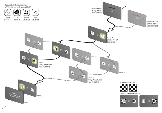
(26) 9. We test this approach using a simple computational interface game where an underlying concept-icon mapping must be discovered in order to complete the task. As mentioned above, the game is structured as a four-level BDT with limited feedback (see Fig. 5.1; see also (W.-T. T. Fu & Anderson, 2006), p198 for a structurally similar design). Each node of the tree represents a decision, and the links between nodes represent the consequences of each decision. The depth of the tree represents the number of sequential choices that are needed to achieve a specific goal. This scenario captures sequential decision-making situations with limited feedback that are pervasive in real world human-computer interface interaction. Furthermore, it allows us to follow the development of expertise as the users discover the rules of the game and deploy different search strategies to solve the task. 2.1. Electrophysiology One of the major substrates of the neurophysiological studies is the electrical activity of the brain. This activity can be sampled using an electrode array, which is placed non-invasively on the scalp. Noninvasive registration is known as Electroencephalogram (EEG), and mainly reflects the sum of postsynaptic potentials of cortical neurons. Stereotyped electrophysiological responses to a stimulus are called Event Related Potentials (ERPs) (S. J. Luck, 2014). ERPs are measured by averaging many trials of the EEG recording to retain the relevant brain’s response to the stimulus while averaging out the random brain activity. As the participant explores the interface, some ERPs are modulated by learning or attentional processes. In the BDT task, these modulations are mainly evoked at each sequential choice, and can be captured at the onset of stimuli such as responses (mouse clicks), feedback presentation, and attentional probes (checkerboard patterns). Checkerboard probes are external stimuli added to the task and are used to sample the early visuospatial attentional components as the P1 and N1 ERPs. This kind of attention is related to the orienting network, which is focused in the prioritization of sensory input by selecting a location (Petersen & Posner, 2012). P1 peak occurs around ⇠70 – 90 milliseconds.

(27) 10. after the onset of the visual stimuli, and N1 peak occurs around ⇠120 – 150 milliseconds respectively. Both components are localized over the lateral occipital scalp. The presentation paradigm used in this work (see Methods section) is similar to the Posner paradigm (Posner, 1980; Posner, Snyder, & Davidson, 1980), where cues are presented lateralized to the left or right positions. Then, the comparison between these ERPs is carried out by comparing the same stimulus when attended or not. Without the behavioral modeling, checkerboard probes comes close to a classical alternative to sample the attentional state of the participants. However, the lack of clear attentional assignations, i.e. what and when an element is or is not attended, makes using this technique difficult in some cases. Mouse responses, which also trigger the presentation of feedback in the last level of the BDT, are also related to visual stimuli. By changing the icons of the binary choice or by presenting feedback of the actions of the participant, a P2 appears. The P2 has a peak located around the centro-frontal area which occurs about 200 ms after the onset of the visual stimuli. Although the characterization of this component is unclear, in the context of visual search tasks its changes could be interpreted as facilitation of attentional deployment toward target locations (Anllo-Vento & Hillyard, 1996; Akyurek & Schubo, 2013); improved task performance (Ross & Tremblay, 2009); and outcome predictability (Polezzi, Lotto, Daum, Sartori, & Rumiati, 2008), among others. Besides the brain processes previously mentioned, this component has been also reported to be modified by feedback (Schuermann, Endrass, & Kathmann, 2012). Thus, it could behave different in the presence of explicit/implicit feedback. Besides the visual ERP components, there are other ERPs related to the decisionmaking process that can be evoked by the mouse response. The Error-Related Negativity (ERN) is a component associated with error processing and occurs within 100 ms of an erroneous response (Gehring, Goss, Coles, Meyer, & Donchin, 1993; Larson, Clayson, & Clawson, 2014). This component is more prominent in frontal and central electrode sites. These errors may be conscious (aware errors) or unconscious (unaware errors), but even.

(28) 11. in correct responses a small negativity could be detected (Shalgi & Deouell, 2012). In the context of BDT choices, the ERN can be understood as the expectations in the outcome of the current decision, which initiates behavioral adjustments in order to optimize the choice selection process (Maier, Yeung, & Steinhauser, 2011). In addition to the ERN and temporally later, other important components of the decision-making process are the P3 and the Late Positive Complex (LPC). P3 component is measured more strongly in the parietal scalp sites, is associated with the evaluation or categorization of a stimulus and has its peak around ⇠300 – 500 ms after stimuli onset. This component has also implications in cognitive workload (Donchin, 1981), and is modulated by the delivery of task relevant information (Polich, 2007). Perhaps the most relevant aspect of the P3 is its widespread use in BCI, mainly due to its robustness (Ahn, Lee, Choi, & Jun, 2014). In the presence of explicit feedback, a fronto-central P3 appears. The feedback-related P3 is suggested to be modulated by information which is motivationally significant or salient (Schuermann et al., 2012). Furthermore, it is also related to the feedback-guided learning by the context updating hypothesis (revisions of the mental model of the task) (San Martı́n, 2012; Donchin & Coles, 1988). Following the P3, the Late Positive Complex is a positive-going ERP component in the temporal window of ⇠500 – 800 ms after stimulus onset, and it is largest in parietal scalp sites. This component is associated with recognition memory (Friedman & Johnson, 2000; Wolk et al., 2006), which is usually divided into two processes: familiarity and recollection. Familiarity is an early process, about ⇠300 – 500 ms, thus it is modulated in the P3 effect. On the other hand, recollection modulates the. LPC, such as in correct source or associative recognition (Curran, Schacter, Johnson, & Spinks, 2001), differences in the remember/known paradigms (Spencer, Abad, & Donchin, 2000), among others. Also, a more parietal LPC topology is associated to post-retrieval processing, as in the strategic processing related to the required task (Ranganath & Paller, 2000). In addition to the previously mentioned ERPs, feedback stimuli are also characterized by the Feedback-Related Negativity (FRN). The FRN is a centro-frontal ERP component associated with the onset of a feedback signaling the outcome of a decision (Miltner,.

(29) 12. Braun, & Coles, 1997; Sallet, Camille, & Procyk, 2013). FRN effects are modulated in decision-making tasks by risk (Schuermann et al., 2012), loss and gain (Liu, Nelson, Bernat, & Gehring, 2014), among other feedback-related properties. In the BDT task, this component is likely to be associated with feedback-guided learning (San Martı́n, 2012; M. M. Walsh & Anderson, 2012), which compares the difference between the obtained and expected value to trigger changes in behavior. By capturing the evolution of the decision-making process over time, the above-mentioned ERPs could reveal how the development of expertise is related (or not) to the attentional resources used by the participant to learn the task. We expect to show these differences when comparing the different stages of the learning process, such as those produced by the formalization of stereotyped search strategies..

(30) 13. 3. HYPOTHESIS We hypothesize that the interaction between a user and an the interface can be described by stereotyped strategies, characterized by a set of predefined actions/decisions and the distinctive use of attentional resources. The level of expertise developed by the user, while exploring the interface, would correlate with changes in the use of such strategies, prompting different curves of performance. Specifically, the dynamics of behavioral and electrophysiological indicators will correlate with distinct patterns over time: a) Behaviorally, as the user explores the interface and learns the underlying mapping between concepts and icons, his or her search process will be characterized by the use of different strategies. Moreover, the development of expertise in the use of the interface will correlate with a decrease in mouse movements variability, likewise, the reaction times and errors will be minimized throughout the course of the experiment. b) Neurophysiologically, the Event Related Potential (ERP) components’ amplitude will be modulated in dependence with the attentional resources allocated by the user, correlating with the user’s individual strategies and the development of expertise..

(31) 14. 4. OBJECTIVES The main objective of this proposal is to experimentally investigate the individual differences in the decision-making process, expertise acquisition, and the attentional dynamics of participants while exploring a novel interface. Using behavioral indicators (participant’s choices, reaction times, mouse tracking, etc) and brain-related ones (event related potentials) we want to characterize the different stages of learning and expertise development. Specifically, we are interested in: a) Studying the deployment of putative search strategies and the development of expertise as a function of task acquaintance. b) Capturing the individual differences of participants in the use of the strategies throughout the task. c) Modeling the decision-making process of participants online (behavioral modeling). d) Predicting the participants’ choices based on the online modeling. e) Studying the electrophysiological changes in relation to the behavioral modeling..

(32) 15. 5. METHODS 5.1. Task In order to represent a Human-Computer Interaction (HCI) scenario that requires learning, we implement a sequential decision making task that participants have to solve through active exploration. The task consists in presenting an instruction to participants and offering them a series of successive binary choices among abstract icons that, depending on the sequence of choices, can lead to either positive or negative feedback (see Figure 5.1 and below for details). In abstract terms, the task is a 4-level BDT where each node of the tree represents a binary decision and the links between nodes represent the consequences of each decision. The depth of the tree represents the number of available sequential choices. This scenario captures sequential decision-making situations with limited feedback that are pervasive in real world human-computer interface interaction (e.g. when drawing cash from an ATM machine). Specifically, participants were presented with a computer screen that had an instruction of the type “verbL1 with a nounL2 an adjectiveL3 nounL4 ” (i.e. “Feed a cat with a small fish”, see inset in Fig. 5.1 and Table 5.1 for more details). Note that because the task was performed by native Spanish speakers, the the final adjective-noun pair is inverted regarding the previous instruction example and would read “Alimenta un gato con un pez pequeño”. After clicking anywhere on this first screen, participants were confronted with the first binary choice (level 1 of the BDT) with two icons located 2.4 to each side of a central fixation spot. Each of the variable words in the instruction had a fixed mapping to an abstract icon and level of the BDT (as indexed by subscripts in the instruction example above), but participants were not informed of this fact. They were instructed to click using the computer mouse on one of the two icons to proceed to the next screen where the next set of two icons was presented (level 2 of the BDT). The overall arrangement of the icons remained constant and only their identity changed according to the specific task mapping. This branching structure was repeated until level 4 was reached. The last level was always.

(33) 16. Figure 5.1. Schematic presentation of the BDT showing one possible instance of the task. Only one screen per level is presented, depending on the icon clicked previously. Highlighted icons along the black continuous lines represent the correct icon-to-concept mapping (see left inset) that, when clicked in the correct sequence, produces a positive feedback. Right inset presents the attentional probes used to sample the attentional state of the participants. the same regardless of the branch because only two possible adjectives were used: “small (pequeño)” or “large (grande)”. Once subjects clicked an icon in level 4 they received feedback informing them whether the path they had chosen was correct. In the case of a negative feedback, subjects had no way of knowing, a priori, at which level they had made the wrong choice. Therefore, they had to discover the mapping based exclusively on their exposure to successive iterations of the task and the feedback received at the end of each chosen path. Importantly, as we chose a set of instructions in which the last binary choice (L4) was always the same, there are a total of 16 different instructions in the BDT. Each instruction (corresponding to a single task instance) was presented repeatedly until.

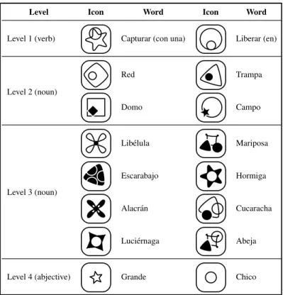
(34) 17. Table 5.1. Icon-concept relationships used in the task. Each row represents a binary choice screen and its related icon-concept mapping. Note that not all binary choices are reachable from one particular icon (except for the fourth level), thus the first icon can only reach the first row (binary choice) of the second level, and the first and second rows of the third level, and so forth. There are 16 possible instances of the structure “(verbL1 ) with a (nounL2 ) an (adjectiveL3 ) (nounL4 )”. Examples of sentences are: “Capturar con una red una lı́belula grande”, “Liberar en el domo un alacrán chico”, “Capturar con una trampa una mariposa chica”, etc. Level Level 1 (verb). Icon. Word. Icon. Word. Capturar (con una). Liberar (en). Red. Trampa. Domo. Campo. Libélula. Mariposa. Escarabajo. Hormiga. Alacrán. Cucaracha. Luciérnaga. Abeja. Grande. Chico. Level 2 (noun). Level 3 (noun). Level 4 (abjective). the participant was able to choose the correct path 5 times in a row before moving onto the next possible instruction. After 15 successive wrong answers, participants were asked whether they wanted to move onto the next task. If they refused, after 10 further wrong answers they were asked again. If they decided to persist in the same task, they only had 5 additional chances to find the correct path else they were forced to move onto the next one. The maximum time allowed to complete the entire task was set to 40 minutes. In addition, to be able to sample the attentional state of participants in the electrophysiological record, checkerboard patterns (see Fig. 5.1 right inset) were added as attentional.

(35) 18. probes across trials. These probes were presented non-simultaneously and centered to the left/right icons. Each probe has a duration of 75 milliseconds, and the temporal separation between them was randomized in the 400–600 milliseconds interval. 5.2. Participants Twenty-two participants were recruited (12 females) of ages ranging from 20 to 32 years old, with a mean age of 26±3 years (mean ± SD). All participants reported normal or corrected-to-normal vision and no background of neurologic or psychiatric conditions.. Participants performed on average 162±51 trials (mean ± SD) during the course of the experiment (range 89-325). Trials are defined as repetitions of an instance of the task,. from the instruction to the feedback after the sequence of choices. Each task instance contains on average 10.79±1.47 trials (mean ± SD). In addition, two groups of participants were defined according to whether they managed to solve the task (learners, N=14) or not (non-learners, N=8) in the allowed time window (40 min). We consider learners all participants who managed to complete the 16 tasks instances, reaching full knowledge of the interface as evidenced by consistent positive feedback. Conversely, the non-learners group is composed by participants who did not complete the task within the time limit, or failed to reach full knowledge of the interface. The study was approved by the Ethics Committee of the School of Psychology of the Faculty of Social Sciences, Pontificia Universidad Católica de Chile. All participants gave written informed consent. The nature of the task was explained to participants upon arrival to the Laboratory. All experiments were performed in the Psychophysiology Lab of the School of Psychology of the same University. Participants sat in a dimly illuminated room, 60 cm away from a 19-inch computer screen with a standard computer mouse in their right hand. All participants were right handed. Prior to staring the task, subjects were fitted with a 32-electrode Biosemi ActiveTwo © digital electroencephalographic (EEG) system, including 4 electrooculographic (EOG) electrodes, two of them placed in the outer canthi of each eye and two above and below the right eye. Continuous EEG was acquired at 2048.

(36) 19. Hz and saved for posterior analysis. Throughout the task, participants were instructed to maintain fixation on a central spot in order to avoid eye-movement related artifacts in the EEG data. All stimuli were presented around fixation or 2.4 to each side of the central fixation spot. This ensured that, despite the instruction to maintain fixation, all participants could easily see all stimuli and perform the task without difficulty in perceptual terms. 5.3. Modeling Framework Subjects (i.e. users) that undertake a decision-making process act based on information that is, in great part, unavailable to an observer (i.e the interface). While perception of the task environment can be available to both, the subject’s prior knowledge, beliefs, preferences and other psychological processes remain hidden from the observer. In other words, the nature of the decision-making processes (i.e. its psychological underpinnings) can only be inferred based on overt actions and, eventually, patterns of overt actions. Importantly, because such hidden information is what makes the difference between different subjects, it represents a natural target for any interface trying to adapt to its current user. To identify these patterns, we develop a Hidden Markov Model (HMM) based approach that capitalizes on the hierarchical structure of behavior. Specifically, (a) inputs captured by the interface such as mouse clicks, correspond to low-level actions; (b) systematic combinations of low-level actions into high-level subroutines correspond to strategies and (c) the expectation of the use of specific strategies or a combination of them corresponds to complex behavior, which we refer as behavioral modeling in this work. In the following sections we will present the modeling framework in detail taking into account each of these concepts. 5.3.1. Low-level Actions vs Strategies The simplest action that can be taken on the BDT is to click one of the two possible icons of the binary choice. We will therefore consider these two as the only low level.

(37) 20. actions for the model. What such low level actions mean or represent, in terms of learning of the BDT, depends on whether the participant is using them in some systematic way to obtain positive feedback (i.e. a strategy). We consider such systematic combination of low-level actions the high-level strategies of the model. Different strategies can be used to search a BDT of the characteristics used here. In the following we model four high-level strategies in the form of well defined search strategies, that account for increasingly sophisticated ways to solve the task: (i) Random Search Strategy: If the participant displays no systematic use of low level actions, we label this as random behavior. In other words, overt actions seem to be unrelated to the task’s demands so that we can only assume ignorance regarding the underlying decision making strategy. (ii) Topological Search Strategy: If the participant shows evidence of searching based exclusively on information regarding the spatial arrangement of the BDT, regardless of the identity of the presented icons (for instance, by choosing to explore from the leftmost to the rightmost branch), we label this as a topological behavior. When clicking based on spatial features, the participant iteratively discards paths of the BDT so that complete knowledge can be obtained only when the 16 paths of the BDT are correctly recognized. Accordingly, as paths share common information, the learning curve of a user invested exclusively in this strategy will grow exponentially as the search space becomes smaller. (iii) Generative Search Strategy: If the participant shows evidence of considering the identity of individual icons to guide her choice of actions to reach positive feedback, we label this as a generative behavior. In other words, it implies a first level of successful mapping between current task instruction and the specific BDT instance that is being explored (i.e. when the participant learns that a given icon means a given concept). When clicking based on generative relationships, the participant discards subtrees of the BDT where it is not possible to reach positive feedback. Complete knowledge of the BDT can be obtained.

(38) 21. when the 16 icons are correctly mapped. All the generative relationships can be learned by being exposed to positive feedback in the 8 paths that contains all of them. Therefore, the learning curve of this strategy is represented by a sigmoid function. (iv) Discriminative Search Strategy: Here the participant uses a generative model, but adds the ability to learn and relate the negative form of a concept-icon relationship (i.e. learn A by a generative association and then label the neighbor as not-A). In other words, the discriminative search strategy is one that predicts concepts that have not yet been seen in the scope of positive feedback. Concepts are deduced from the context and the understanding of the rules of how the interface works. When clicking based on discriminative relationships, the participant can prune the BDT subtrees more aggressively to obtain positive feedback. As in the generative case, complete knowledge of the BDT can be obtained when the 16 icons are correctly mapped. However, all discriminative relationships can now be learned by being exposed to positive feedback in the 4 paths that contains all of them. Accordingly, the learning curve of this strategy is represented by a sigmoid function that is steeper than in the generative case. Each of the above models has an initial domain of action that corresponds to the set of actions that can be performed on the BDT according to the strategy’s rules. Once exploration of the interface is underway, the initial domain of action of each strategy will necessarily change. This can happen because the user learns something about the specific task instance he is currently solving, or because he learns something about the overall structure of the interface. It is therefore necessary to define criteria that, according to each strategy’s rules, allow one to update their domain of action depending on local (taskinstance) and global (task-structure) knowledge. Local updates criteria will coincide with the rules of the topological strategy for all systematic strategies, because according to our hierarchical definition, the simplest way to discard places of the BDT systematically is using topological information. Conversely, for global updates –and for the sake of simplicity– we will define knowledge in terms of optimal behavior, (i.e. learning places.

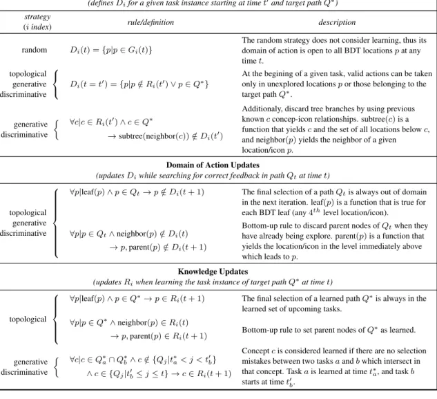
(39) 22. or concepts of the task instances by repeating the correct path 5 times in a row). Tab. 5.2 presents the formal definition of the domain of action Di and both updating schemes for each strategy si . Table 5.2. Formal definitions of the strategies are presented according to their initial domain, domain of action updates (task instance learning), and knowledge updates (task structure learning). Initialization of the Domain of Action (defines Di for a given task instance starting at time t0 and target path Q⇤ ) strategy (i index). rule/definition. random 8 topological < generative : discriminative generative discriminative. ⇢. description. Di (t) = {p|p 2 Gi (t)}. The random strategy does not consider learning, thus its domain of action is open to all BDT locations p at any time t.. Di (t = t0 ) = {p|p 2 / Ri (t0 ) _ p 2 Q⇤ }. At the begining of a given task, valid actions can be taken only in unexplored locations p or those belonging to the target path Q⇤ .. 8c|c 2 Ri (t0 ) ^ c 2 Q⇤. ! subtree(neighbor(c)) 2 / Di (t0 ). Additionaly, discard tree branches by using previous known c concep-icon relationships. subtree(c) is a function that yields c and the set of all locations below c, and neighbor(p) yields the neighbor of a given location/icon p.. Domain of Action Updates (updates Di while searching for correct feedback in path Qt at time t) 8 > > > > > > > topological > < generative > discriminative > > > > > > > :. topological. generative discriminative. 8 > > > > < > > > > : ⇢. 8p|leaf(p) ^ p 2 Qt ! p 2 / Di (t + 1). 8p|p 2 Qt ^ neighbor(p) 2 / Di (t). ! p, parent(p) 2 / Di (t + 1). The final selection of a path Qt is always out of domain in the next iteration. leaf(p) is a function that is true for each BDT leaf (any 4th level location/icon). Bottom-up rule to discard parent nodes of Qt when they have already being explore. parent(p) is a function that yields the location/icon in the level immediately above which leads to p.. Knowledge Updates (updates Ri when learning the task instance of target path Q⇤ at time t) 8p|leaf(p) ^ p 2 Q⇤ ! p 2 Ri (t + 1) 8p|p 2 Q⇤ ^ neighbor(p) 2 Ri (t). ! p, parent(p) 2 Ri (t + 1). 8c|c 2 Q⇤a \ Q⇤b ^ c 2 / {Qj |t⇤a < j < t0b }. ^ c 2 {Qj |t0b  j  t} ! c 2 Ri (t + 1). The final selection of a learned path Q⇤ is always in the learned set of upcoming tasks. Bottom-up rule to set parent nodes of Q⇤ as learned. Concept c is considered learned if there are no selection mistakes between two tasks a and b which intersect in that concept. Task a is learned at time t⇤a , and task b starts at time t0b ..

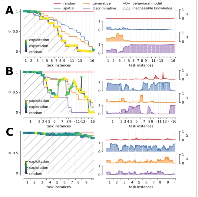
(40) 23. To track the BDT knowledge of the specific strategy si , we define ↵i as a measure of what still needs to be mapped (place or concept) of the BDT at a given time t : ↵i (t) = 1. |Ri (t)| |Gi (t)|. (5.1). where Ri (t) is the set of learned choices, Gi (t) is the set of all distinct choices in the strategy’s domain, and | · | is the number of elements of a given set. This parameter is the complement of the specific learning curve of each strategy. Specifically, ↵i = 1 indicates complete lack of knowledge about the interface, and ↵i = 0 indicates full knowledge. Note that high-level strategies evolve according to the user’s iterative interactions with the task. For instance, if the participant does not show evidence of learning any path, the learning curve of each strategy is a straight constant line at ↵i = 1. When feedback becomes available (i.e. when the participant reaches the end of a path producing either a correct or incorrect answer), we ask each model how such observation changes or violates its expected probabilities regarding the nature of future feedback. As long as no learning is involved, all active models will answer equally to this query. However, as evidence of learning becomes available, each model will restrict the domain of possible future actions that are consistent with what the model predicts the participant’s knowledge should be. A topological model will label as a mistake any repetition of a path that previously gave positive feedback in the context of a different instruction. A generative model will label as mistakes actions that are inconsistent with a successful icon-concept mapping for which there is prior evidence. The discriminative model inherits the restrictions imposed by the generative model, but will also consider mistakes as those actions that do not take into account not-A type knowledge that the participant should have, given the history of feedback. An important consequence of the above is that strategies can yield the probability of clicking a given icon of the BDT without further training or modeling at any moment throughout the task. It is worth noting that defining all possible strategies to solve the BDT is not necessary. To delimit the knowledge level of the participant, only the lower and higher bounds of the.

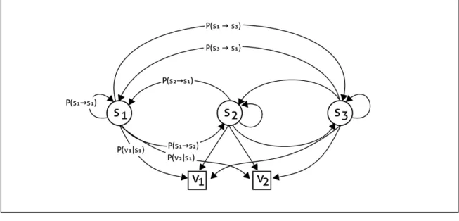
(41) 24. problem must be defined and more strategies in-between will only increase the framework’s resolution. In the BDT case used here, the lower bound is necessarily the random strategy. The upper bound is set by the discriminative strategy because it is the best possible strategy to solve the BDT task (i.e. it requires the least exposure to positive feedback). Accordingly, we make the assumption that at any given moment, the user has all strategies at his disposal but that overt behavior is best captured by a weighted mix of them. We call this level the behavioral model of the framework. 5.3.2. Behavioral Modeling Once the high-level strategies are defined, we turn to modeling the expectation about the use of a specific strategy or a combination of them by the participant. Such behavioral model is composed by a modular architecture of the four possible strategies, which interact between them in a HMM-like structure. This modular architecture has the advantage of modeling complex strategies as if they were a single abstract state in the behavioral model. Formally, a HMM is defined by a finite set of hidden states, s1 , s2 , . . . , sn , and each time a relevant information arises (e.g. feedback) the system moves from one state s(t) = si to another s(t + 1) = sj (possibly the same). The transition probabilities, P (si ! sj ), determine the probability of transiting between states: P (si ! sj ) = P (s(t + 1) =. sj |s(t) = si ). The observable information of the process is a finite set of distinct observations, v1 , v2 , . . . , vm , and a probabilistic function of the states. Accordingly, each observation has an emission probability P (vk |si ), k 2 {1, . . . , m}, of being seen under a state si . As the system must start somewhere, it is necessary to define an initial probability. distribution of the states: wi = P (s(t = 0) = si ), i 2 {1, . . . , n}. Given that the sets of hidden states and observations are defined a priori, the only values to estimate are the initial distribution and the transition and emission probabilities. Each strategy therefore takes the role of a hidden state at the behavioral level, which then yields the probability distribution of each observation for each trial. See Fig. 5.2 for a graphical example of a HMM..

(42) 25. Figure 5.2. Graphical representation of a Hidden Markov Model. A HMM with 3-states ({s1 , s2 , s3 }) and 2 observations ({v1 , v2 }). Labels for the transition and emission probabilities of the state s1 are included in the diagram. In our framework, the states si will be represented by a set of strategies that contains search behaviors (strategy models) to solve the task. The transition probabilities will determine the probability that a participant changes her or his search behavior depending on her/his level of expertise, and the observable information of the process will be determined by the sequential choice outcome. 5.3.2.1. Emission Probabilities Although the task can yield positive and negative feedback, an observer can interpret these observations in different ways depending on the situation. While positive feedback is unambiguous (a hit observation), negative feedback can have two different connotations: it is a mistake if, given previous actions, the observer is warranted to assume that the participant should have had the knowledge to avoid performing the action that produced such outcome. Observing such feedback will therefore mean evidence in favor of random behavior. Else, negative feedback is consistent with exploratory search behavior prior to the.

(43) 26. first positive feedback and, accordingly, not considered a mistake. The set of observations V is therefore defined as: V = {mistake, explore, hit}. Since strategies are sensitive to the context, their emission probabilities change as the participant makes choices. At each sequence step, we calculate the emission probabilities within the subtree of possible future choices. Considering the last choice of the participant as the root of the subtree, we enumerate all possible future paths of actions Q, defining the following sets at step t: Hi (t) = {Q|(8a 2 Q)[a 2 Di (t)] ^ (9a 2 Q)[a 2 / Q⇤ ]}. (5.2). Hi⇤ (t) = {Q|(8a 2 Q)[a 2 Q⇤ ]}. (5.3). where a represents a specific action needed to generate path Q, and Q⇤ the target path. Hi (t) is the set of all paths that do not violate the strategy’s rules, while simultaneously allowing the exploration of available choices. Hi⇤ (t) is the set of paths that lead to positive feedback. Thus, emission probabilities for strategy si are defined as follows:. P (V |s(t) = si ) =. 8n > < 0,. |Hi⇤ (t)| |Hi (t)| , |Hi (t)|+|Hi⇤ (t)| |Hi (t)|+|Hi⇤ (t)|. > :{1, 0, 0},. o. ,. if |Hi (t)| > 0 _ |Hi⇤ (t)| > 0 otherwise (5.4). The first case represents emission probabilities for those strategies that, given their rules, allow for future exploration or exploitation. In the second case, when the rules of the strategy cannot explain the current actions, the emission probabilities are fixed to explain mistakes. This is also the case for the random strategy, which is assumed when the observer has no knowledge about the participant’s strategy. 5.3.2.2. Transition Probabilities It is possible, but not necessary, that a participant moves progressively through each of the increasingly complex strategies as he learns the structure of the task. Although.

(44) 27. such progression may seem as discrete steps (i.e. first using a topological strategy and then abandoning it altogether when conceptual knowledge becomes available), it is most likely that at any given moment of the task, the participant’s strategy will fall somewhere in between, being better represented by a mix of strategy models. This is precisely the distribution captured by the behavioral model. To estimate it, it is necessary to model the interactions between strategies si , in terms of transition probabilities and relative weights. To obtain the transition probabilities we use a voting scheme based on emission probabilities, where each strategy distributes its own P (V |si ) depending on the ability of the. strategy to explain a specific type of observation. Thus, for each observation v 2 V we define the set of best explanatory strategies of v as follows:. Bv (t) = {si |si 2 arg max P (v|si )}. (5.5). si. t Then, every step t in which the participant performs an action, transition links lij between. strategies si and sj gain votes according to the following rules: 8 > >1, if si 2 Bv (t) ^ i = j > > < X t 1 lij = P (v|si ) , if sj 2 Bv (t) ^ si 2 / Bv (t) |Bv (t)| > > v2V > > :0, otherwise. (5.6). These rules represent three cases: (a) Any strategy that belongs to Bv (t) strengthens its self-link, not sharing its P (v|si ) with other strategies. (b) Strategies that do not belong to Bv (t) generate links to those that best explain the observation v, losing their P (v|si ) in equal parts to those that best explain v. (c) Strategies that do not explain v or do not belong to Bv (t) do not receive votes for observing v. In the case of the random strategy, its emission probabilities are fixed to {1, 0, 0},. therefore the above rules do not generate links with other strategies in the case of exploring or exploiting the BDT knowledge. In order to overcome this limitation, we define the set of strategies that can leave the random strategy as those that do not see the current action.

(45) 28. as a mistake, plus the random strategy itself: U (t) = {si |P (mistake|si ) = 0} [ {srandom } Then, the links from random strategy are voted as: 8 > 1 <1, if sj 2 U (t) t lrandom j = |U (t)| > :0, otherwise Note that malized.. P. v. (5.7). (5.8). P (v|si ) = 1 for each strategy, thus the vote sharing scheme is always nor-. The value of these links represent only what happens at the current time. The participant’s actions, however, can be tracked historically by defining an observation window of the process ⌧ , which modulates the weight of the votes over time. Therefore, at time t, the amount of cumulative votes L between strategies i and j is defined by: Pt q lij ⌧ (n) Lij (t) = Pn=0 = P (si ! sj ) t ⌧ (n) n=0 Here we define ⌧ as a Gaussian function with a standard deviation of. (5.9) steps, normalized. to a maximum of 1 at the current time t: ⌧ (n) = e. (n t)2 2 2. (5.10). The result is a set of directed interactions (i.e. transition probabilities) among different strategies, storing historical information of the participants’ behavior. 5.3.2.3. Weights Optimization Weights represent the probability distribution across strategy models at each iteration. Once emission and transition probabilities are known, weights are updated by comparing the cost, in terms of probabilities, to start in some strategy and end in the best transition link that explains an observation type. This allows us to compare the transition that best.

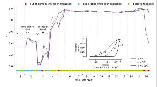
(46) 29. represents the current state of the behavioral model (to where the system is moving) for a specific observation, and how much it costs for each model to reach that point. The cost, in terms of probability of moving from the state sk to sj (which could be the same), given an observation v 2 V , is represented by P (sk ! sj )P (v|sj ). Note that there may be more than one best transition for the system. Accordingly, we define set of best transition links as: {(sk , sj )|arg max P (sk ! sj )P (v|sj )}. (5.11). sk ,sj 2 M. where M represents the set of all strategy models. Eq. 5.11 implies that the behavioral model identifies the transition from sk to sj as one of the most representative in case of observing v at time t. In case more than one best transition exists, the most convenient path is optimized. Then, for an initial state si , the cost of reaching the best transition link is defined as the path that maximizes the following probability: Lii (t)P (v|si )P (sa ! sb )P (v|sb ) · · · P (sk ! sj )P (v|sj ) We use Lii as the prior for the initial probability wi (t), so that models with wi (t. (5.12) 1) = 0. can be incorporated in the optimization at time t. Note that Eq. 5.12 is equivalent to the Viterbi path constrained to a fixed observation v. Then, the weight of strategy si at time t + 1 is represented by the total cost for the set of observations V : wi (t + 1) =. X. v2V. wi (t)P (v|si ) · · · P (sk ! sj )P (v|sj )⌧v (t). (5.13). where ⌧v (t) yields the relevance of observation v in the total cost function, given an observation window ⌧ (such as defined in Eq. 5.10): 8 > t <1, if v(t = n) = v X ⌧v (t) = ⌧ (n) > :0, otherwise n=0. (5.14).

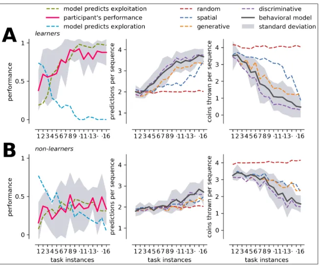
(47) 30. The most likely observation at time step v(t) is defined by consensus regarding the observation with the best average emission probabilities: X. v(t) = arg max v2V. P (v|si ). (5.15). si 2M. Finally, in order to obtain a probability distribution over the search strategies, each weight is normalized by the coefficient W defined as: W =. X. wi (t + 1). (5.16). i2M. Note that if two or more models have the same domain of action (e.g. both concept-based strategies have the same domain of action for target path Q⇤ ), we consider only the one with greatest knowledge. Otherwise the normalization is unfair to the other models. 5.3.2.4. Learning Curve Each strategy’s individual knowledge of the BDT, ↵i , can be combined with its respective weight wi to produce a mixture of basal strategies ↵⇤ . This is accomplished by a weighted sum: ↵⇤ (t) =. X. ↵i (t)wi (t). (5.17). i2M. Recall that ↵i is the complement of the specific learning curve of each strategy. Therefore, the approximate learning curve of a given participant can be obtained as: 1. ↵⇤ .. 5.3.2.5. Predicting Participants’ Choices As the models’ weights are known previous to icon selection, we can build a Mixture of Experts (Jacobs, Jordan, Nowlan, & Hinton, 1991) where search strategy models become the experts that must answer the question “Which icon is the participant most likely to click in the next step?”. Because each model can produce any of two possible actions, i.e clicking on the left or the right icon, the most probable next choice at step t will be the.

(48) 31. one that has the largest support as expressed by the weighted sum rule of the ensemble: 8 > <1, if a 2 hi (t) X arg max µa (t) = wi (t) (5.18) > a 2 {left,right} : i2M 0, otherwise. where hi (t) represents the expert-prediction of the strategy i. Prediction can be based on dichotomous decisions or random selection. Dichotomous decisions occur when there is only one possible action in the strategy’s domain of action so that it will be selected with probability equal to 1. Alternatively, when both possible actions belongs to the strategy’s domain (i.e. have equal probability of being selected) or when neither of the actions belongs to the domain (i.e. the strategy is in the inactive set), a coin is tossed to choose at random (50/50 guess). It is worth noting that the prediction capability of each strategy depends on the size of its domain of action. Strategies with wider exploratory behaviors often have larger domains, and consequently, less predictive power due to the number of paths that can be selected. This aspect is captured by the number of 50/50 guesses, because, as mentioned above, whenever the strategy has more than one equally likely possibility of action, it must choose at random. This does not mean that the strategy itself is failing to capture the participants’ choice of action, but that the conditions are ambiguous enough to keep looking for the correct path. 5.3.3. Scores To better visualize the search process of participants (and groups of participants), we introduce three scores. As any sequence of choices can be the consequence of different degrees of expertise (from fully random behavior to goal-directed exploitation), we define a scale where we assign points depending on the most likely observation v(t) that yields the behavioral modeling (Eq. 5.15) at each step of a sequence of choices Q..