Search for supersymmetry at root 8=8 TeV in final states with jets and two same sign leptons or three leptons with the ATLAS detector
50
0
0
Texto completo
(2) Contents 1. 2 ATLAS detector and data sample. 3. 3 Simulated event samples. 4. 4 Physics object reconstruction. 5. 5 Event selection 5.1 Signal regions. 7 7. 6 Background estimation 6.1 Background estimation methods 6.1.1 Prompt lepton background 6.1.2 Fake-lepton background 6.1.3 Background from lepton charge mis-measurement 6.2 Systematic uncertainties on the background estimation 6.3 Cross-checks of the data-driven background estimates 6.4 Validation of background estimates. 9 9 9 9 10 11 12 13. 7 Results and interpretation 7.1 Model-independent upper limits 7.2 Model-dependent limits 7.2.1 Gluino-mediated top squarks 7.2.2 Gluino-mediated (or direct) first- and second-generation squarks 7.2.3 Direct bottom squarks 7.2.4 MSUGRA/CMSSM, bRPV, GMSB and mUED. 16 19 19 20 22 24 25. 8 Conclusion. 27. The ATLAS collaboration. 34. 1. Introduction. Supersymmetry (SUSY) [1–9] is a generalisation of space-time symmetries that predicts new bosonic partners for the fermions and new fermionic partners for the bosons of the Standard Model (SM). If R-parity is conserved [10, 11], SUSY particles are produced in pairs and the lightest supersymmetric particle (LSP) is stable. In a large variety of models, 0 the LSP is the lightest neutralino (χ̃1 ) and provides a possible candidate for dark matter.. –1–. JHEP06(2014)035. 1 Introduction.
(3) The coloured superpartners of quarks and gluons, the squarks (q̃) and gluinos (g̃), could be produced in strong interaction processes at the Large Hadron Collider (LHC) and decay via 0 0 cascades ending with a stable χ̃1 . The undetected χ̃1 would result in substantial missing miss ). The rest of the cascade would yield transverse momentum (pmiss and its magnitude ET T ˜ final states with multiple jets and possibly leptons arising from the decay of sleptons (`), the superpartners of leptons, or W , Z and Higgs (h) bosons. If R-parity is violated (RPV), miss . the LSP is not stable, which would lead to similar signatures but with lower, or no, ET. In this paper, events containing multiple jets and either two leptons of the same electric charge (same-sign leptons, SS) or at least three leptons (3L) are used to search for strongly produced supersymmetric particles. Throughout this paper, the term leptons (`) refers to electrons and/or muons only. Signatures with SS or 3L are predicted in many SUSY scenarios. Gluinos produced in pairs or in association with a squark can lead to SS signatures when decaying to any final state that includes leptons because gluinos are Majorana fermions. Squark production, directly in pairs or through g̃g̃ or g̃ q̃ production with subsequent g̃ → q q̃ decay, can also lead to SS or 3L signatures when the squarks decay in cascades involving top quarks (t), charginos, neutralinos or sleptons, which subsequently ±(∗) χ̃0 , χ̃0 → h/Z (∗) χ̃0 , or `˜ → `χ̃0 , respectively. Similar decay as t → bW , χ̃± 1 j i j i → W signatures are also predicted by non-SUSY models such as minimal Universal Extra Dimensions (mUED) [20]. Since this search benefits from low SM backgrounds, it allows miss , increasing the sensitivity to the use of relatively loose kinematic requirements on ET scenarios with small mass differences between SUSY particles (compressed scenarios) or where R-parity is violated. This search is thus sensitive to a wide variety of models based on very different assumptions. The analysis uses pp collision data from the full 2012 data-taking period, corresponding √ to an integrated luminosity of 20.3 fb−1 collected at s=8 TeV, and significantly extends the reach of previous searches performed by the ATLAS [21] and CMS [22–25] Collaborations. Five statistically independent signal regions (SR) are designed to cover the SUSY processes illustrated in figure 1. Two signal regions requiring SS and jets identified to originate from b-quarks (b-jets) are optimised for gluino-mediated top squark and direct bottom 0 The charginos χ̃± 1,2 and neutralinos χ̃1,2,3,4 are the mass eigenstates formed from the linear superposition of the SUSY partners of the Higgs and electroweak gauge bosons (higgsinos, winos and binos). 1. –2–. JHEP06(2014)035. In the Minimal Supersymmetric Standard Model [12–14] (MSSM), the scalar partners of right-handed and left-handed quarks, q̃R and q̃L , can mix to form two mass eigenstates, q̃1 and q̃2 , where q̃1 denotes the lighter particle. This mixing effect is proportional to the corresponding SM fermion masses and therefore is more important for the third generation. Furthermore, SUSY can solve the hierarchy problem of the SM (also referred to as the naturalness problem) [15–19] if the masses of the gluinos, higgsinos1 (the superpartners of Higgs bosons) and top squarks (t̃) are not heavier than the O(TeV) scale. A light lefthanded top squark also implies that the left-handed bottom squark (b̃L ) may be relatively light because of the SM weak-isospin symmetry. As a consequence, the lightest bottom squark (b̃1 ) and top squark (t̃1 ) could be produced with relatively large cross sections at the LHC, either directly in pairs or through g̃g̃ production followed by g̃ → b̃1 b or g̃ → t̃1 t decays (gluino-mediated production)..
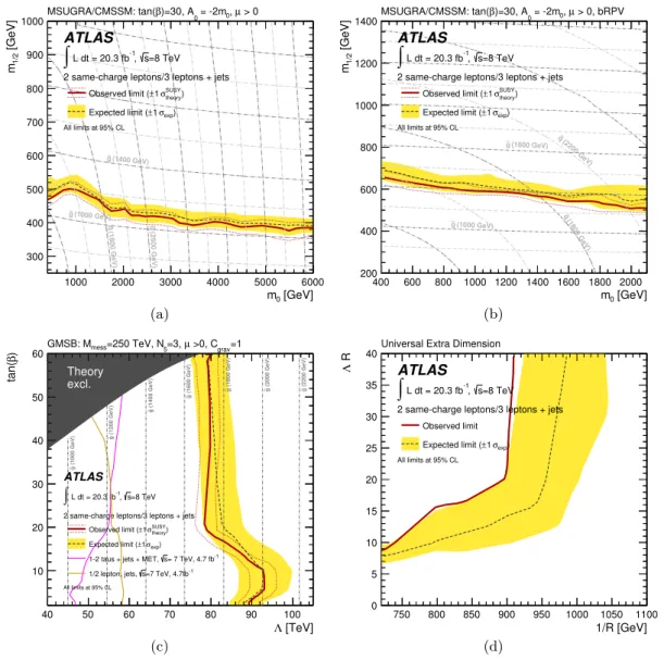
(4) g̃. t t̃1 t χ̃01 b χ̃± 1. q̃. gluino-mediated top squark → b χ̃± 1. c χ̃01. gluino-mediated top squark → c χ̃01. bs. gluino-mediated top squark → b s (RPV). W q q̃ (∗) ± q ′ χ̃1. q̃. q q̃ (∗) q χ̃02. b̃1. t χ̃± 1. g̃. W ±(∗) χ̃01. ±(∗) χ̃0 2. W ±(∗) χ̃01. ˜l± ν, l± ν̃ ˜ll, ν̃ν. W ±(∗) χ̃01. Z (∗) χ̃01. gluino-mediated (or direct) squark → q ′ W Z χ̃01 gluino-mediated squark → q ′ W χ̃01 gluino-mediated (or direct) squark → sleptons. direct bottom squark → t χ̃± 1. Figure 1. Overview of the SUSY processes considered in the analysis. The initial supersymmetric ¯ ¯ The notation q (q̃) refers to quark particles are always produced in pairs: pp → g̃g̃, b̃b̃ or q̃ q̃. 0 (squark) of the first or second generation. The slepton and sneutrino decay as `˜ → `χ̃1 and 0 ν̃ → ν χ̃1 , respectively. Leptons in the final state can arise from the decay of any W or Z bosons or sleptons that are produced. The charge-conjugate processes are also considered.. squark production. These are complemented with a signal region requiring a b-jet veto, optimised for the gluino-mediated production of first- and second-generation squarks. Two signal regions requiring 3L are designed for scenarios characterised by multi-step decays. Backgrounds with prompt SS or 3L events arising from rare SM processes, such as tt̄W , tt̄Z, W ± W ± and W Z, are estimated with Monte Carlo simulations. Backgrounds from hadrons mis-identified as leptons, leptons originating from heavy-flavour decays, electrons from photon conversions, and electrons with mis-measured charge are estimated with datadriven methods. The background predictions are cross-checked with alternative methods and tested with data in validation regions chosen to be close in phase space to the signal regions. The probability (p-value) of the background-only hypothesis is then estimated independently in each signal region. To maximise the sensitivity of the analysis across the entire phase space, a simultaneous fit is performed in all signal regions to place modeldependent exclusion limits on several SUSY benchmark scenarios.. 2. ATLAS detector and data sample. ATLAS is a multi-purpose detector [26] designed for the study of pp and heavy-ion collisions at the LHC. It provides nearly full solid angle2 coverage around the interaction point. 2. ATLAS uses a right-handed coordinate system with its origin at the nominal interaction point (IP) in the centre of the detector and the z-axis along the beam pipe. The x-axis points from the IP to the centre. –3–. JHEP06(2014)035. g̃. gluino-mediated top squark → t χ̃01.
(5) 3. Simulated event samples. Simulated events are used to model the SUSY signal, optimise the event selection requirements, compute systematic uncertainties and estimate some of the SM backgrounds with prompt same-sign lepton pairs or three leptons. These include top quark(s) plus bosons (W/Z/H), diboson (W ± W ± , W Z, ZZ, W H, ZH), triboson (W W W , W ZZ, ZZZ) and tt̄tt̄ production. Other sources of background such as tt̄, W/Z+jets, W γ, W + W − , tt̄γ and single-top production are estimated with data-driven methods described in section 6. Samples of tt̄V +jets (V = W, Z), tt̄W W , single top quark plus a Z boson, V V V +jets and tt̄tt̄ are generated with MadGraph-5.1.4.8 [28] interfaced to Pythia-6.426 [29]. Alternative tt̄V +jets samples generated with Alpgen-2.14 [30] interfaced with Herwig6.520 [31] and Jimmy-4.31 [32] are employed to estimate the sensitivity of the analysis to Monte Carlo modelling. The Pythia-8.165 [33] generator is used to model tt̄H production, for which the Higgs boson mass is set to 125 GeV. The W Z and W ± W ± processes are modelled using Sherpa-1.4.1 [34] with matrix elements producing up to three final-state partons. The ZZ process is generated with Powheg-1.0 [35] interfaced to Pythia-8.165. Monte Carlo modelling systematic uncertainties for the ZZ process are estimated using two sets of aMc@nlo [36] samples where next-to-leading-order (NLO) matrix elements are matched to either Pythia-6.426 or Herwig-6.520 with Jimmy-4.31 parton showers according to the Mc@nlo formalism [37]. Monte Carlo samples of tt̄ events are used to provide corrections to the data-driven background estimates, described in section 6.1, for kinematic regions where the sample size is not sufficient to measure the tt̄ contriof the LHC ring, and the y-axis points upward. Cylindrical coordinates (r,φ) are used in the transverse plane, φ being the azimuthal angle around the beam pipe. The pseudorapidity is defined in terms of the polar angle θ as η = − ln tan(θ/2).. –4–. JHEP06(2014)035. Charged particles are tracked by the inner detector, which covers the pseudorapidity region |η| < 2.5. In order to measure their momenta, the inner detector is embedded in the 2 T magnetic field of a thin superconducting solenoid. Sampling calorimeters span the pseudorapidity range up to |η| = 4.9. High-granularity liquid-argon (LAr) electromagnetic calorimeters are present up to |η| = 3.2. Hadronic calorimeters with scintillating tiles as active material cover |η| < 1.7 while LAr technology is used for hadronic calorimetry from |η| = 1.5 to |η| = 4.9. The calorimeters are surrounded by a muon spectrometer. The magnetic field is provided by air-core toroid magnets. Three layers of precision gas chambers track muons up to |η| = 2.7 and muon trigger chambers cover the range |η| ¡ 2.4. A three-level trigger system is used to select interesting events for storage and subsequent analysis. The data set, after the application of beam, detector and data quality requirements, has an integrated luminosity of 20.3 ± 0.6 fb−1 . The luminosity is measured using techniques similar to those described in ref. [27] with a preliminary calibration of the luminosity scale derived from beam-overlap scans performed in November 2012. The number of pp interactions occurring in the same bunch crossing varies between approximately 10 and 30 with an average of 20.7 for this data set..
(6) 4. Physics object reconstruction. Jets are reconstructed from topological clusters [56, 57] formed from calorimeter cells by using the anti-kt algorithm [58, 59] with a cone size parameter of 0.4 implemented in the FastJet package [60]. Jet energies are corrected [57] for detector inhomogeneities and the non-compensating response of the calorimeter using factors derived from test beam, cosmic ray and pp collision data, as well as from the detailed Geant4 detector simulation. The impact of multiple overlapping pp interactions is accounted for using a technique,. –5–. JHEP06(2014)035. bution directly in data. Four different samples are used: Powheg-1.0 interfaced with Pythia-6.426, Powheg-1.0 interfaced with Herwig-6.520 and Jimmy-4.31, [email protected] interfaced with Herwig-6.520 and Jimmy-4.31 and Alpgen-2.14 interfaced with Herwig-6.520 and Jimmy-4.31. The NLO CT10 [38] parton distribution function (PDF) set is used with Sherpa, Powheg and Mc@nlo while the CTEQ6L1 [39] PDF set is used with MadGraph, Pythia and Alpgen. The predicted background yields are obtained by normalising the simulated samples to theoretical cross sections from the most precise available calculations [40–42]. The SUSY signal samples are generated with Herwig++2.5.2 [43] or MadGraph5.1.4.8 interfaced with Pythia-6.426, in both cases using the PDF set CTEQ6L1. Signal cross sections are calculated to next-to-leading order in the strong coupling constant, adding the resummation of soft gluon emission at next-to-leading-logarithmic accuracy (NLO+NLL) [44–48]. The cross section and its uncertainty are taken from an envelope of cross-section predictions using different PDF sets and factorisation and renormalisation scales, as described in ref. [49]. The mUED samples are generated with Herwig++2.5.2 using the CTEQ6L1 PDF set and the leading-order cross section from Herwig++. The parton shower parameters of the simulated samples were tuned to match ATLAS data observables sensitive to initial- and final-state QCD radiation, colour reconnection, hadronisation, and multiple parton interactions. The tuned parameter set AUET2 [50] is used with Pythia 6, Herwig 6 and Pythia 8 (except that the tune P2011C [51] is used for the Powheg + Pythia tt̄ sample), and the set UEEE3 [52] is used with Herwig++. The effect of additional proton-proton collisions in the same or neighbouring bunch crossings, called “pile-up”, is modelled by overlaying minimum-bias events, simulated with Pythia-8.160 using the AUET2 tune, onto the original hard-scattering event. Simulated events are weighted to reproduce the observed distribution of the average number of collisions per bunch crossing in data. Monte Carlo samples are passed through a detector simulation [53] based on Geant4 [54] or on a fast simulation using a parametric response to the showers in the electromagnetic and hadronic calorimeters [55] and Geant4-based simulation elsewhere. Simulated events are reconstructed with the same algorithms as data. Corrections derived from data control samples are applied to account for differences between data and simulation for the lepton trigger and reconstruction efficiencies, momentum scale and resolution, and for the efficiency and mis-tag rate for tagging jets originating from b-quarks..
(7) –6–. JHEP06(2014)035. based on jet areas, that provides an event-by-event and jet-by-jet pile-up correction [61]. Selected jets are required to have transverse momentum pT > 40 GeV and |η| < 2.8. The identification of b-jets is performed using a neural-network-based b-tagging algorithm [62] with an efficiency of 70% in simulated tt̄ events. The probabilities for mistakenly b-tagging a jet originating from a c-quark or a light-flavour parton are approximately 20% and 1% [63, 64], respectively. The kinematic requirements on b-jets are pT > 20 GeV and |η| < 2.5. Signal jets and b-jets are selected independently, hence b-jets with pT > 40 GeV are included in both jet and b-jet multiplicities. Electron candidates are reconstructed using a cluster in the electromagnetic calorimeter matched to a track in the inner detector. Preselected electrons must satisfy the “medium” selection criteria described in ref. [65], re-optimised for 2012 data, and fulfil pT > 10 GeV, |η| < 2.47 and requirements on the impact parameter of the track. Muon candidates are identified by matching an extrapolated inner detector track to one or more track segments in the muon spectrometer [66]. Preselected muons must fulfil pT > 10 GeV and |η| < 2.5. Signal leptons are defined by requiring tighter quality criteria and increasing the pT threshold to 15 GeV. Signal electrons must satisfy the “tight” selection criteria [65]. In addition, for both the signal electrons and muons, isolation requirements based on tracking and calorimeter information and impact parameter requirements are applied. The electron track isolation discriminant is computed as the summed scalar pT of additional tracks inside p a cone of radius ∆R = (∆η)2 + (∆φ)2 = 0.2 around the electron. The tracks considered must originate from the same vertex associated with the electron and have pT > 0.4 GeV. The electron calorimeter isolation discriminant is defined as the scalar sum of the transverse energy, ET , of topological clusters within a cone of radius ∆R = 0.2 around the electron cluster and is corrected for any contribution from the electron energy and pile-up. The muon track and calorimeter isolation discriminants are the same as the ones used for electrons, except for the isolation cone radius being ∆R = 0.3 and calorimeter cells around the muon extrapolated track being used for the calorimeter isolation discriminant. For leptons with pT < 60 GeV, both track and calorimeter isolation are required to be smaller than 6% and 12% of the electron’s and muon’s pT , respectively. For leptons with pT > 60 GeV, an upper limit of 3.6 GeV and 7.2 GeV is imposed on both the calorimeter and track isolation requirements for electrons and muons, respectively. The track associated with the electron or muon candidate must have a longitudinal impact parameter z0 satisfying |z0 sin θ| < 0.4 mm and fulfil the requirement for the significance of the transverse impact parameter, d0 , of |d0 /σ(d0 )| < 3. The track parameters z0 and d0 are defined with respect to the reconstructed primary vertex. For events with multiple vertices along the beam P 2 axis, the vertex with the largest pT of associated tracks is taken as the primary vertex. Furthermore, the primary vertex must be made of at least five tracks with pT > 0.4 GeV and its position must be consistent with the beam spot envelope. Ambiguities between the reconstructed jets and leptons are resolved by applying the following criteria sequentially. Jets with a separation ∆R < 0.2 from an electron candidate are rejected. Any lepton candidate with a distance ∆R < 0.4 to the closest remaining jet is discarded. If an electron and a muon have a separation ∆R < 0.1, the electron is discarded. For these requirements, jets with pT > 20 GeV and preselected leptons are considered..
(8) miss , is constructed The missing transverse momentum vector, pmiss with magnitude ET T as the negative of the vector sum of the calibrated transverse momenta of all muons and electrons with pT > 10 GeV, jets with pT > 20 GeV and calorimeter energy clusters with |η| < 4.9 not assigned to these objects [67].. 5. Event selection. 5.1. Signal regions. The signal regions are determined with an optimisation procedure using simulated events from the simplified models illustrated in figure 1. The data are divided into two mutually exclusive SS and 3L samples. In the SS sample, the two highest-pT leptons must have the same electric charge and fulfil pT > [20,15] GeV, and there must be no other signal lepton with pT > 15 GeV. In the 3L sample, the three highest-pT leptons must fulfil pT > [20,15,15] GeV, respectively. No requirements on the total electric charge are applied to this sample. Good sensitivity to the signatures in all signal models is obtained by defining five non-overlapping signal regions with selection requiremiss ; jet and b-jet multiplicities (N ments based on the following kinematic variables: ET jets and Nb−jets ); effective mass meff computed from all signal leptons and selected jets as P ` P miss + meff = ET pT + qpjet T ; transverse mass computed from the highest-pT lepmiss as m = miss (1 − cos[∆φ(` , pmiss )]); and invariant mass m ton (`1 ) and ET 2p`T1 ET 1 T T `` computed with opposite-charge same-flavour leptons. As detailed in table 1, the selection requirements of the five signal regions are:. • SR3b: SS or 3L events with at least five jets and at least three b-jets; miss and large m ; • SR0b: SS events with at least three jets, zero b-jets, large ET T. –7–. JHEP06(2014)035. miss and non-isolated single-lepton Events are selected using a combination (logical OR) of ET miss and dilepton triggers. The thresholds applied to ET and the leading and subleading lepton pT are lower than those applied offline to ensure that trigger efficiencies are constant miss is 80 GeV. The p thresholds in the phase space of interest. The trigger threshold for ET T for single-lepton triggers are 60 GeV and 36 GeV for electrons and muons, respectively. The dilepton triggers feature lower thresholds in pT , down to 12 GeV for electrons and 8 GeV for muons, allowing events with multiple soft leptons to be kept. The efficiencies of miss -only triggers in the phase space of interest are close to 100%. The electron triggers ET reach efficiencies above 95% and muon triggers have efficiencies between 75% and 100%, being lowest in the region |η| < 1.05. Events from non-collision backgrounds are rejected using dedicated quality criteria [57]. Events of interest are selected if they contain at least two leptons passing the requirements described in section 4 and if the highest-pT lepton satisfies pT > 20 GeV. Events with a leading pair of leptons having an invariant mass m`` < 12 GeV are removed. This requirement rejects events with pairs of energetic leptons from decays of heavy hadrons and has negligible impact on the signal acceptance..
(9) SR. Leptons. Nb−jets. Other variables. Additional requirement on meff. SR3b. SS or 3L. ≥3. Njets ≥ 5. meff >350 GeV. miss > ET. SR0b. SS. =0. Njets ≥ 3,. SR1b. SS. ≥1. miss > 150 GeV, Njets ≥ 3, ET. meff >700 GeV. —. miss < 150 GeV, Njets ≥ 4, 50 < ET. meff >400 GeV. miss > 150 GeV, SR3b veto Njets ≥ 4, ET. meff >400 GeV. 150 GeV,. meff >400 GeV. mT > 100 GeV. SR3Llow. 3L. mT >100 GeV, SR3b veto Z boson veto, SR3b veto. 3L. —. Table 1. Definition of the signal regions (see text for details).. • SR1b: similar to SR0b, but with at least one b-jet; miss and Z boson veto; • SR3Llow: 3L events with at least four jets, small ET miss . • SR3Lhigh: 3L events with at least four jets and large ET. The Z boson veto in SR3Llow rejects events with any opposite-charge same-flavour lepton combination of invariant mass 84 < m`` < 98 GeV. An additional meff requirement is applied to maximise the expected significance of selected SUSY models in each signal region. This requirement on meff is relaxed in the model-dependent limit-setting procedure described in section 7.2. The signal regions are all mutually exclusive. An SR3b veto, which rejects events satisfying the SR3b selection, is included in the definition of other signal regions that would otherwise have a small overlap with SR3b. Each signal region is motivated by different SUSY scenarios and different SUSY parameter settings. The SR3b signal region targets gluino-mediated top squark scenarios resulting in signatures with four b-quarks. This signal region does not require large values miss or m , hence it is sensitive to compressed scenarios with small mass differences or of ET T to unstable LSPs. The SR0b signal region is sensitive to gluino-mediated and directly produced squarks of the first and second generations, which do not enhance the production of b-quarks. Third-generation squark models resulting in signatures with two b-quarks, such 0 as direct bottom squark or gluino-mediated top squark → cχ̃1 production, are targeted by SR1b. The 3L signal regions have no requirement on the number of b-jets. They target scenarios where squarks decay in multi-step cascades, such as gluino-mediated (or direct) 0 squark → q 0 W Z χ̃1 and gluino-mediated (or direct) squark → sleptons (see figure 1). The miss requirement, SR3Llow, targets compressed regions of the phase signal region with low ET space where SUSY decay cascades would produce off-shell W and Z bosons. Backgrounds from Z boson production in association with jets are suppressed by a Z boson veto. Models miss and on-shell vector bosons are targeted by SR3Lhigh. Hence no Z boson with large ET veto is applied in this signal region, but Z + jets backgrounds are suppressed by the larger miss requirement. ET. –8–. JHEP06(2014)035. SR3Lhigh.
(10) 6. Background estimation. Searches in SS and 3L events are characterised by low SM backgrounds. Three main classes of backgrounds can be distinguished. They are, in decreasing order of importance for this search: (1) prompt multi-leptons, (2) “fake” leptons, which denotes hadrons misidentified as leptons, leptons originating from heavy-flavour decays, and electrons from photon conversions, and (3) charge mis-measured leptons. 6.1. Prompt lepton background. The background with prompt leptons arises mainly from W or Z bosons, decaying leptonically, produced in association with a top-antitop quark pair where at least one of the top quarks decays leptonically, and from diboson processes (W Z, ZZ, W ± W ± ) in association with jets. The tt̄V and diboson backgrounds are dominant for signal regions with and without b-jets, respectively. The prompt multi-lepton backgrounds are estimated from Monte Carlo samples normalised to NLO calculations as described in section 3. The rarer processes tt̄H, single top quark plus a Z boson, tt̄tt̄ and V V V +jets, each of which constitutes at most 10% of the background in the signal regions, are also included. The production of tt̄W W , W H and ZH (where the Higgs boson decay can produce isolated leptons from W , Z or τ ) were verified to give a negligible contribution to the signal regions. 6.1.2. Fake-lepton background. The number of events with at least one fake lepton is estimated using a data-driven method. A fake-enriched class of “loose” leptons is introduced, composed of preselected leptons (defined in section 4) with pT > 15 GeV failing the signal lepton selection. If the ratio of the number of signal leptons to the number of loose leptons is known separately for prompt and fake leptons, the number of events with at least one fake lepton can be predicted. For illustration, when only pairs of leptons are considered, the equation that relates the number of events with signal (S) or loose (L) leptons to the number of events with prompt (P ) or fake (F ) leptons: . NSS NP P N N SL PF =Λ· NLS NF P NLL NF F. , . (6.1). where the first and second indices refer to the leading and subleading lepton of the pairs, can be inverted to obtain the expected number of events with at least one fake lepton. The matrix Λ is given by ε1 ε2 ε1 ζ 2 ζ1 ε 2 ζ1 ζ2 ε (1 − ε ) ε1 (1 − ζ2 ) ζ1 (1 − ε2 ) ζ1 (1 − ζ2 ) 1 2 Λ= (6.2) , (1 − ε1 )ε2 (1 − ε1 )ζ2 (1 − ζ1 )ε2 (1 − ζ1 )ζ2 (1 − ε1 )(1 − ε2 ) (1 − ε1 )(1 − ζ2 ) (1 − ζ1 )(1 − ε2 ) (1 − ζ1 )(1 − ζ2 ). –9–. JHEP06(2014)035. 6.1.1. Background estimation methods.
(11) 6.1.3. Background from lepton charge mis-measurement. Background from charge mis-measurement, commonly referred to as “charge-flip”, consists of events with two opposite-sign leptons for which the charge of a lepton is mis-identified. Such events constitute a background only for the SS signal regions. The dominant mechanism of charge mis-identification is due to the radiation of a hard photon from an electron followed by an asymmetric conversion, for which the electron with the opposite charge has the larger pT (e± → e± γ → e∓ e± e± ). The probability of mis-identifying the charge of a muon is determined in simulation to be negligible in the kinematic range relevant to this analysis. The electron charge-flip background is estimated using a fully data-driven tech-. – 10 –. JHEP06(2014)035. where ε1 and ε2 (ζ1 and ζ2 ) are the ratios of the number of signal and loose leptons for the leading and subleading prompt (fake) leptons, respectively. This analysis employs a generalised matrix method where an arbitrary number of loose leptons can be present in the event. For example, an event containing three leptons that pass, in decreasing order of pT , the signal-loose-signal selections is considered a SS signal event if the first and third lepton have the same charge. In addition, this event is included in the fake-lepton background calculation for 3L events since the second lepton passes only the loose selections. In general, eqs. (6.1)–(6.2) are adapted by dynamically adjusting the size of the matrix Λ according to the number of loose leptons in the event under study. No upper limit on the number of loose leptons is set. Each event is employed in all its possible incarnations (signal and/or as part of the background calculation) as illustrated in the example above, but is only included in one of the signal regions, which are exclusive by definition. The efficiencies ε and ζ are measured in data as a function of the lepton pT and η. The prompt lepton efficiencies are determined from a data sample enriched with prompt leptons from Z → `+ `− decays, obtained by requiring 80 < m`` < 100 GeV. As the background is dominated by events with one real lepton and one fake lepton, the fake-lepton efficiencies are measured from a data set enriched with one prompt muon (by requiring it to pass the signal lepton selection and pT > 40 GeV) and an additional fake lepton (by requiring it to pass the loose selections). The fake electron background has contributions from heavy flavour decays, as well as from conversions and fake pions. The fake-electron efficiency is therefore determined from two samples of SS eµ events to be sensitive to the different types of fake electrons, one with a b-jet veto and another with at least one b-jet. The fake-muon efficiency is determined from a sample of same-sign dimuon events where at least two jets with pT > 25 GeV are required. The event yields in these control regions are corrected for the contamination of prompt SS using Monte Carlo simulation. The eµ SS control regions are also corrected for the presence of charge mis-measured electrons using the likelihood fit method described in section 6.1.3, but applied to loose electrons. The contamination from signal events is verified to be negligible in the same-sign eµ and µµ control regions. The size of the data sample is not sufficient to allow the extraction of the fake-lepton efficiencies for muons with pT > 40 GeV or for events with at least three b-jets. For these events the fake-lepton efficiencies obtained from data in similar kinematic regions, i.e. muons with 25 < pT < 40 GeV or events with at least one b-jet, are employed and corrected with extrapolation factors obtained from the tt̄ Monte Carlo samples..
(12) 6.2. Systematic uncertainties on the background estimation. The systematic uncertainties on the sources of prompt SS and 3L events arise from the Monte Carlo simulation and normalisation of these processes. The cross sections used to normalise the Monte Carlo samples are varied according to the uncertainty on the theory calculation, i.e. 22% for tt̄W [40] and tt̄Z [41] and 7% for diboson production (computed with MCFM [42], considering scales, parton distribution functions and αs uncertainties). Normalisation uncertainties between 35% and 100% are applied to processes with smaller contributions. Uncertainties caused by the limited accuracy of the tt̄V +jets and diboson+jets Monte Carlo generators are estimated by varying the renormalisation and factorisation scales and the QCD initial- and final-state radiation used to generate these samples. Additional Monte Carlo modelling uncertainties are included, such as the limited number of hard jets that can be produced from matrix element calculations in the MadGraph+Pythia and Sherpa samples, which is the largest modelling uncertainty for the diboson+jets process, and the difference between the predictions of various Monte Carlo generators such as MadGraph versus Alpgen, which is the largest modelling uncertainty for the tt̄V +jets process. Monte Carlo simulation-based estimates also suffer from detector simulation uncertainties. These are dominated by the uncertainties on the jet energy scale and the b-tagging efficiency. The jet energy scale uncertainty is derived using a combination of simulations, test beam data and in situ measurements [57, 68]. Additional contributions from the jet flavour composition, calorimeter response to different jet flavours, pile-up and b-jet calibration uncertainties are taken into account. The efficiency to tag real and fake b-jets is corrected in Monte Carlo events by applying b-tagging scale factors, extracted in tt̄ and dijet samples, that compensate for the residual difference between data and simulation [62, 64, 69]. The associated systematic uncertainty is computed by varying the scale factors within their uncertainty. Uncertainties in the jet energy resolution are obtained 3. An asymmetric window around the Z boson mass is chosen because charge-flip electrons lose more energy in the detector than electrons for which the charge is properly reconstructed.. – 11 –. JHEP06(2014)035. nique. The charge-flip probability is extracted in two Z boson control samples, one with same-sign electron pairs and the other with opposite-sign electron pairs. The invariant mass of these same-sign and opposite-sign electron pairs is required3 to be between 75 GeV and 100 GeV. Background events are subtracted using the invariant mass sidebands. A likelihood fit is employed which takes as input the numbers of same-sign and opposite-sign electron pairs observed in the sample. The charge-flip probability is a free parameter of the fit and is extracted as a function of the electron pT and η. The probability of electron charge-flip varies from approximately 10−4 to 10−2 in the range 0 ≤ |η| ≤ 2.47 and 15 < pT < 200 GeV, increasing with electron |η| and pT . The event yield of this background in the signal regions is obtained by applying the measured charge-flip probability to data regions with the same kinematic requirements as the signal regions but with oppositesign lepton pairs. The contamination from fake leptons and signal events is found to be negligible in these opposite-sign control regions..
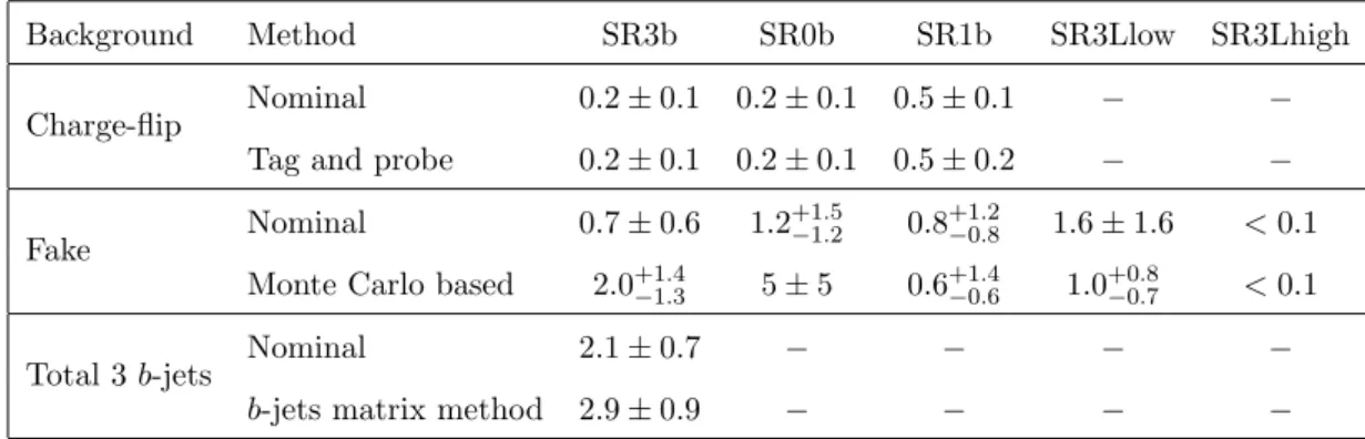
(13) Background Charge-flip. Fake. Method. SR3b. SR0b. SR1b. SR3Llow. SR3Lhigh. Nominal. 0.2 ± 0.1. 0.2 ± 0.1. 0.5 ± 0.1. −. −. Tag and probe. 0.2 ± 0.1. 0.2 ± 0.1. 0.5 ± 0.2. −. −. Nominal. 0.7 ± 0.6. 1.2+1.5 −1.2. 0.8+1.2 −0.8. 1.6 ± 1.6. < 0.1. Monte Carlo based Total 3 b-jets. 2.0+1.4 −1.3. 5±5. 0.6+1.4 −0.6. 1.0+0.8 −0.7. < 0.1. Nominal. 2.1 ± 0.7. −. −. −. −. b-jets matrix method. 2.9 ± 0.9. −. −. −. −. with an in situ measurement of the jet response asymmetry in dijet events [70]. Other uncertainties on the lepton reconstruction [65, 71], calibration of calorimeter energy clusmiss calculation [67], luminosity [27] and ters not associated with physics objects in the ET simulation of pile-up events are included but have a negligible impact on the final results. The fake-lepton background uncertainty includes the statistical uncertainty from the SS control regions, the dependence of the fake-lepton efficiency on the event selections and the contamination of the SS control regions by real leptons. Uncertainties on the extrapolation of the fake-lepton efficiency to poorly populated kinematic regions are estimated by comparing the prediction of different tt̄ Monte Carlo samples. For the charge-flip background prediction, the main uncertainties originate from the statistical uncertainty of the charge-flip probability measurements and the background contamination of the sample used to extract the charge-flip probability. 6.3. Cross-checks of the data-driven background estimates. Three alternative methods were developed to cross-check the background estimates from data-driven methods. The results are summarised in table 2, showing the background predictions for the nominal methods, described in section 6.1, and the cross-check methods described below. In each case consistent predictions are obtained, but with generally larger uncertainties for the alternative methods. For the electron charge-flip background, a simpler “tag and probe” method is employed which selects electron pairs with an invariant mass consistent with a Z boson decay. One electron is required to have |η| < 1.37. Its charge is assumed to be measured correctly. The charge-flip probability is extracted as a function of pT and η of the other electron, which is required to be in the pseudorapidity region 1.52 < |η| < 2.47, by computing the ratio of same-sign to opposite-sign pairs. The charge-flip probability for central electrons is extracted by requiring that both electrons are in the same pT and η region. This chargeflip probability is applied in the same manner as the nominal charge-flip probability, as described in section 6.1, to obtain a prediction in the signal regions. The fake-lepton background estimate were cross-checked with a simulation-based technique. This method relies on kinematic extrapolation from control regions, with low jet. – 12 –. JHEP06(2014)035. Table 2. Comparison of the predicted number of background events in the signal regions using the nominal and cross-check methods. Both the statistical and systematic uncertainties are included..
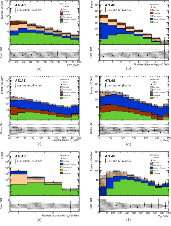
(14) 6.4. Validation of background estimates. The data-driven background estimates are based on control regions that employ less strinmiss gent requirements on the jet and b-jet multiplicities, total transverse energy and/or ET than the signal regions. To ensure their validity in the signal regions, the background estimates are validated in events with kinematic properties closer to the signal regions. This is first performed by individually probing each of the kinematic variables used to define the signal regions in events containing a same-sign lepton pair. The event is not rejected if it contains more than two leptons. Several relevant kinematic distributions are studied for each lepton channel and for events with and without a b-jet. No significant discrepancies are observed. Some example distributions are shown in figure 2. Each of the background types (fake electron, fake muon, charge-flip electron and prompt SS) is dominant, and thus validated directly, in particular regions of the kinematic phase space examined by these SS validation regions. However, the prompt SS contributions are typically dominated by inclusive W Z production, while the prompt SS or 3L background in the signal regions is expected to be dominated by tt̄V and W Z events produced in association with several hard jets. The Monte Carlo modelling of these rare processes is tested in a further set of dedicated validation regions. The event selections are presented in table 3. They are based on the object definitions described in section 4, and. – 13 –. JHEP06(2014)035. miss , to the signal regions that require high jet multiplicity and E miss . multiplicity and ET T The separate control regions are characterised by the presence or the absence of a b-jet, and by the flavours of the two leading leptons. Backgrounds with prompt leptons are obtained from Monte Carlo simulation as described in section 6.1.1. Backgrounds with fake leptons and charge-flip electrons are obtained from Monte Carlo simulations normalised to match data in the control regions. The normalisation is done using five multipliers. One multiplier is used to correct the rate of electron charge mis-identifications. The other four corrections are for processes producing either fake electrons or muons that originate from b-jets or light jets. The background in the SR3b region is expected to be completely dominated by events with at least one light or charm jet mis-tagged as a b-jet, i.e. a fake b-tag. A crosscheck of the background estimate in this signal region is performed by determining the number of events with at least one fake b-tag. A generalised matrix method applied to the estimation of fake b-tags is used, similar to that described in section 6.1.2, with the following differences. Loose leptons are replaced by jets, signal leptons by b-tagged jets, and the different tight/loose incarnations are combined in each event. The efficiency for fake b-tags is estimated in a tt̄-enriched sample with at least one signal lepton, at least four jets miss < 200 GeV. with pT > 20 GeV, of which at least two must be b-tagged, and 100 < ET The efficiency for fake b-tags is calculated using the additional b-jets found in each event after subtracting contamination from events with three or more real b-jets (such as tt̄bb̄). The efficiency to tag real b-jets is determined independently of the efficiency for fake b-tags, as described in refs. [62, 69]. The efficiencies for tagging real and fake b-jets are fed into the matrix method to predict the background in SR3b. Small contributions from processes with three real b-jets are estimated from simulation..
(15) 5 Same-sign ee. ATLAS. ∫ L dt = 20.3 fb ,. 104 10. Events. Events / 25 GeV. 10. -1. >0 b-jets Data. s=8 TeV. SM Total. 10 10. 5. 10. 4. 10. 3. Charge-flip. 3. Fake leptons. 6. ATLAS. Same-sign ee. ∫ L dt = 20.3 fb , -1. Data. s=8 TeV. SM Total Charge-flip Fake leptons Diboson + Triboson. Diboson + Triboson Top + X. 102. Top + X. 102. 10. 10 1. 1 20. 40. 60. 80. 100. 120. 140. 160. miss. 2. Missing transv. momentum E. T. 200. [GeV]. 1 40. 60. 80. 100. 120. 140. 160 180 200 miss ET [GeV]. (a) 10. 6. 10. 5. Same-sign eµ. ATLAS. ∫. 0 b-jet -1. Data. L dt = 20.3 fb , s=8 TeV. SM Total Fake leptons. 104. Diboson + Triboson Charge-flip. 10. 3. 10. 2. 1. 2. 3. 4. 5. 6 T. 0. 1. 2. 3. 4 5 6 7 Number of jets with p >40 GeV T. (b). Top + X. 7. Number of jets with p >40 GeV. 1 0. Events / 25 GeV. 20. 0. 2. 10. 5 Same-sign eµ. ATLAS. ∫. 104 10. 3. 10. 2. 0 b-jet -1. Data. L dt = 20.3 fb , s=8 TeV. SM Total Fake leptons Diboson + Triboson Charge-flip Top + X. 10. 10 1. 1 40. 60. 80. 100. 120. 140. 2. 160. 180. Leading lepton p [GeV] T. 1 40. 60. 80. 100. 120. 6. 10. 5. Data -1. L dt = 20.3 fb , s=8 TeV. SM Total Diboson + Triboson. 104 10. 3. 10. 2. 100. 150. 200. 250. 300. Transverse mass (lead lepton) [GeV]. 1 0 0. 50. 100. 150. 200. 250 300 mT [GeV]. (d). Same-sign µµ. ATLAS. ∫. 50. T. (c) 10. 0. 2. 140 160 180 200 Leading lepton p [GeV]. Events / 100 GeV. 0 20. Events. 200. Data / SM. Data / SM. 20. Fake leptons Top + X. 104 Same-sign µµ. ATLAS 10. ∫. 3. >0 b-jets -1. Data. L dt = 20.3 fb , s=8 TeV. SM Total Fake leptons Diboson + Triboson. 102. Top + X. Charge-flip. Charge-flip. 10. 10 1. -0.5. 0. 0.5. 1. 2. 1.5. 2. 2.5. 3. 3.5. Number of bjets with p >20 GeV T. 1 0. 0. 1. (e). 2 3 Number of b-jets with p >20 GeV T. Data / SM. Data / SM. 1. 0. 100. 200. 300. 400. 500. 2. 600. 700. 800. 900. 1000. Effective mass (inclusive) [GeV]. 1 0 0. 100. 200. 300. 400. 500. 600. 700. 800. 900 1000 meff [GeV]. (f). miss Figure 2. Distributions of kinematic variables in SS background validation regions: (a) ET for events with at least one b-jet and (b) number of jets for the ee channel, (c) leading lepton pT for events with no b-jet and (d) transverse mass, mT , for events with no b-jet for the eµ channel, and (e) number of b-jets and (f) effective mass, meff , for events with at least one b-jet for the µµ channel. The statistical and systematic uncertainties on the background prediction are included in the uncertainty band. The last bin includes overflows. The lower part of the figure shows the ratio of data to the background prediction.. – 14 –. JHEP06(2014)035. 0 0. Events / 20 GeV. 180. Data / SM. Data / SM. 0.
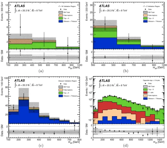
(16) Leptons (pT > 20 GeV). Njets. Nb−jets. miss (GeV) ET. mT (GeV). Additional cuts. tt̄W. SS µµ. ≥ 1 (30 GeV). =2. 20 to 120. > 80. −. tt̄Z. 3L. ≥ 2 (40 GeV). 1 or 2. 20 to 120. −. meff > 300 GeV,. Background Probed. Z boson mass W Z+jets. ≥ 2 (20 GeV). SS µµ. Veto. 20 to 120. −. > 100. ∫. t t + W Validation Region Data. -1. L dt = 20.3 fb , s = 8 TeV. SM Total Fake leptons Top + X. 8. Diboson + Triboson. 30 25. 10. 2. 5. 1 200. 300. 400. 500. 600. 700. 800. (a) 100. 80. ATLAS. ∫. 900. L dt = 20.3 fb , s = 8 TeV. SM Total Fake leptons Top + X. 60. Diboson + Triboson. SM Total. Top + X Diboson + Triboson. meff [GeV]. 1 0 300. 1000. Data. Data. 2. meff [GeV]. Diboson Validation Region -1. Data / SM. 4. meff [GeV]. ∫. t t + Z Validation Region -1. L dt = 20.3 fb , s = 8 TeV. Fake leptons. 15. 2. ATLAS. 20. 6. 0 100. Events / 100 GeV. Events / 233 GeV. 10. ATLAS. 400. 500. 600. 700. 800. 900. 105. ATLAS. ∫. 104. 1000. meff [GeV]. (b) Events / 100 GeV. Events / 300 GeV. Data / SM. 12. Opposite-sign, ≥ 3 b-jets Data. -1. L dt = 20.3 fb , s = 8 TeV. SM Total Top + X. 103. Z + jets Fake leptons Diboson + Triboson. 102 40. 10 1. 20. 2 1 0 100. 200. 300. 400. (c). 500. 600. 700. Data / SM. Data / SM. 10-1 meff [GeV]. 800. meff [GeV]. 2 0 1. 0. 0. 200. 400. 600. 800. 1000. 1200. 200. 400. 600. 800. 1000. 1200. 1400. 1400 meff [GeV]. (d). Figure 3. Effective mass (meff ) distributions for the (a) tt̄W , (b) tt̄Z, (c) W Z+jets and (d) OS plus three b-jets validation regions. The statistical and systematic uncertainties on the background prediction are included in the uncertainty band. The last bin includes overflows. The lower part of the figure shows the ratio of data to the background prediction.. impose different jet pT thresholds and require pT > 20 GeV for the leptons to increase the rejection of fake-lepton events. The tt̄W and W Z+jets validation regions employ only SS µµ events to avoid fake-electron events. The signal contamination is verified to be negligible for the tt̄Z and W Z+jets validation regions and at most 25% for the tt̄W validation. – 15 –. JHEP06(2014)035. Table 3. Definition of the validation regions for rare SM backgrounds. The required jet pT threshold is indicated in parentheses under the column Njets . The Z boson mass cut demands at least one opposite-charge same-flavour lepton pair satisfying 84 < m`` < 98 GeV..
(17) region for non-excluded SUSY models. The meff distributions of these validation regions are shown in figures 3(a)–3(c). The prediction is observed to agree with the data, therefore validating the Monte Carlo modelling of these rare SM processes. The SR3b signal region receives a large contribution of tt̄V events where at least one light or charm jet is mis-tagged as a b-jet. The Monte Carlo modelling of this mis-tag rate is validated in a large opposite-sign dilepton sample where at least three b-tags are required. This sample is dominated by dilepton tt̄ events where the third b-jet is mistagged. Figure 3(d) shows the meff distribution in this sample, for which the Monte Carlo simulation prediction is shown to describe the data.. Results and interpretation. Figure 4 shows the effective mass distribution of the observed data events and SM predictions for the five signal regions, after all selections except the one on meff . SUSY models of particular sensitivity to each signal region are also shown for illustration purposes. These models, illustrated in figure 1 and described in section 7.2, are: gluino-mediated top squark → bs (RPV) with gluino mass of 945 GeV and top squark mass of 417 GeV for ± 0 SR3b; gluino-mediated squark → q 0 W χ̃1 with gluino mass of 705 GeV, χ̃1 mass of 450 GeV 0 0 and χ̃1 mass of 225 GeV for SR0b; gluino-mediated top squark → cχ̃1 with gluino mass of 0 700 GeV, top squark mass of 400 GeV and χ̃1 mass of 380 GeV for SR1b; gluino-mediated ± 0 squark → sleptons with gluino mass of 905 GeV, χ̃2 and χ̃1 masses of 705 GeV, slepton 0 and sneutrino masses of 605 GeV and χ̃1 mass of 505 GeV for SR3Llow; and direct bottom χ̃± χ̃0 squark → tχ̃± 1 with bottom squark mass of 450 GeV, 1 mass of 200 GeV and 1 mass of 60 GeV for SR3Lhigh. The numbers of observed data events and expected background events in the five signal regions, after the application of the additional requirements on meff , are presented in table 4. Expected signal yields from the SUSY models appearing in figure 4 are also shown. Diboson production in association with jets is a large source of background for signal regions that do not require the presence of b-jets, namely SR0b, SR3Llow and SR3Lhigh. In SR1b and SR3b, which require one or more b-jets, the largest background contribution arises from tt̄V events. The background from fake leptons is particularly significant in signal miss , such as SR3b and SR3Llow. Background regions with no or low requirements on ET from electron charge mis-identification is small in all SS signal regions, and not applicable in the 3L signal regions. The level of agreement between the background prediction and data is quantified by computing the p-value for the number of observed events to be consistent with the background-only hypothesis, denoted by p(s = 0) in table 4. To do so, the number of events in each signal region is described using a Poisson probability density function (pdf). The statistical and systematic uncertainties on the expected background values are modelled with nuisance parameters constrained by a Gaussian function with a width corresponding to the size of the uncertainty considered. The data and predicted background agree well for SR3b, SR3Llow and SR3Lhigh. No events with total electric charge of ±3 are observed in the 3L signal regions. For SR0b and SR1b, small excesses are observed corresponding. – 16 –. JHEP06(2014)035. 7.
(18) Events / 300 GeV. Events / 655 GeV. SR3b Region. ATLAS. 7. ∫. Data SM Total. -1. L dt = 20.3 fb , s = 8 TeV. Fake leptons. 6. Charge flip Top + X. 4. SR0b Region. ATLAS 20. ∫. 18. Data SM Total. -1. L dt = 20.3 fb , s = 8 TeV. Fake leptons Charge flip Top + X. 16. Diboson + Triboson ~~ g-g production ~ ~ ~ g→ t1t, t1→ bs (RPV) ~ ~ (g, t1) = (945, 417) GeV. 5. 22. Diboson + Triboson 0 0 ~~ g g → qqq’q’WW ∼ χ∼ χ 1 1 0 ± m(∼ χ ) = 2 m(∼ χ). 14. 1. 1. ~ (g, χ0) = (705, 225) GeV. 12. 1. 10 3. 8 6. 2. 4 1 2 400. 600. 800. 1000. 1200. 1400 meff [GeV]. 400. 600. 800. SR1b Region. 30. ATLAS. Data. ∫L dt = 20.3 fb , -1. 1200. 1400 meff [GeV]. (b) SR0b Events / 472 GeV. Events / 400 GeV. (a) SR3b. 1000. SM Total. s = 8 TeV. Fake leptons. 25. Charge flip Top + X Diboson + Triboson 0 ~~ ~ g-g production, g→ tc+∼ χ 1 0 ~ m(∼ χ ) = m(t1) - 20 GeV 1 ~ ~ (g, t1) = (700, 400) GeV. 20. 18 SR3Llow Region. ATLAS 16. Data. ∫L dt = 20.3 fb , -1. SM Total. s = 8 TeV. Fake leptons Charge flip. 14. Top + X Diboson + Triboson ~~ g-g decays via sleptons 0 0 ~~ χ + neutrinos g g → qqq’q’ll(ll)∼ χ ∼. 12. 1. 15. 1. ~ (g, χ0) = (905, 505) GeV. 10. 1. 8 6. 10. 4 5 2. 400. 600. 800. 1000. 1200. 1400 meff [GeV]. Events / 722 GeV. (c) SR1b. 300. 400. 500. 600. 700. 800. 900. 1000. 1100 1200 meff [GeV]. (d) SR3Llow SR3Lhigh Region. ATLAS. 6. Data. ∫L dt = 20.3 fb , -1. SM Total. s = 8 TeV. Fake leptons Charge flip. 5. Top + X Diboson + Triboson ~ ~ b1-b1 production ~ 0 ± b → t∼ χ , m(∼ χ ) = 60 GeV. 4. 1. 1. 1. ~ (b1, χ±) = (450, 200) GeV 1. 3. 2. 1. 400. 600. 800. 1000. 1200. 1400. 1600 1800 meff [GeV]. (e) SR3Lhigh. Figure 4. Effective mass (meff ) distributions in the signal regions SR3b, SR0b, SR1b, SR3Llow and SR3Lhigh, used as input for the exclusion fits. The statistical and systematic uncertainties on the background prediction are included in the uncertainty band. The last bin includes overflows. Signal expectations from SUSY models of particular sensitivity in each signal region are shown for illustration (see text).. – 17 –. JHEP06(2014)035. 200.
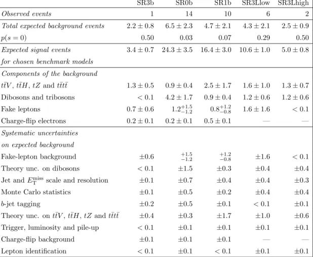
(19) Observed events Total expected background events p(s = 0). SR3b. SR0b. SR1b. SR3Llow. SR3Lhigh. 1. 14. 10. 6. 2. 2.2 ± 0.8. 6.5 ± 2.3. 4.7 ± 2.1. 4.3 ± 2.1. 2.5 ± 0.9. 3.4 ± 0.7. 24.3 ± 3.5. 16.4 ± 3.0. 10.6 ± 1.0. 5.0 ± 0.8. 1.3 ± 0.5. 0.9 ± 0.4. 2.5 ± 1.7. 1.6 ± 1.0. 1.3 ± 0.7. 0.7 ± 0.6. 1.2+1.5 −1.2. 0.8+1.2 −0.8. 1.6 ± 1.6. < 0.1. —. —. 0.50. Expected signal events for chosen benchmark models. 0.03. 0.07. 0.29. 0.50. Components of the background tt̄V , tt̄H, tZ and tt̄tt̄ Fake leptons Charge-flip electrons. < 0.1. 4.2 ± 1.7. 0.9 ± 0.4. 1.2 ± 0.6. 1.2 ± 0.6. 0.2 ± 0.1. 0.2 ± 0.1. 0.5 ± 0.1. ±0.6. +1.5 −1.2. +1.2 −0.8. ±1.6. < 0.1. ±0.4. ±0.4. ±0.3. Systematic uncertainties on expected background Fake-lepton background Theory unc. on dibosons Jet and. miss ET. scale and resolution. Monte Carlo statistics b-jet tagging Theory unc. on tt̄V , tt̄H, tZ and tt̄tt̄. < 0.1 ±0.1. ±0.1. ±0.2. ±0.4. Trigger, luminosity and pile-up. < 0.1. Charge-flip background. ±0.1. Lepton identification. < 0.1. ±1.5. ±0.3. ±0.5. ±0.2. ±0.7. ±0.5. ±0.3. ±0.1. ±0.1. ±0.1. ±0.4. ±0.4. ±0.4. ±0.4. ±0.1. < 0.1. ±0.1. ±0.1. ±1.7. ±1.0. ±0.1. —. < 0.1. ±0.1. ±0.1. ±0.6. ±0.1 —. ±0.1. Table 4. Number of observed data events and expected backgrounds and summary of the systematic uncertainties on the background predictions for SR3b, SR0b, SR1b, SR3Llow and SR3Lhigh. The p-value of the observed events for the background-only hypothesis is denoted by p(s = 0). By convention, the p(s = 0) value is truncated at 0.50 when the number of observed data events is smaller than the expected backgrounds. The expected signal events correspond to the SUSY models considered for each signal region in figure 4 with their experimental uncertainties. The breakdown of the systematic uncertainties on the expected backgrounds, expressed in units of events, is also shown. The individual uncertainties are correlated and therefore do not necessarily add up in quadrature to the total systematic uncertainty.. to 1.8 and 1.5 standard deviations, respectively. The significance is calculated using the uncertainty on the total expected background yields quoted in table 4 and the Poissonian uncertainty of the total expected background value. If SR0b and SR1b are combined, the significance of the excess becomes 2.1 standard deviations. Table 4 also presents the breakdown of uncertainties on the background predictions described in section 6.2. For all signal regions the background uncertainty is dominated by the statistical uncertainty on the expected number of background events. The largest systematic uncertainties arise from the estimation of the fake-lepton probability and from the theoretical predictions for diboson+jets and tt̄V +jets processes. Uncertainties on the predicted background event yields are quoted as symmetric, except where the negative error reaches zero predicted events, in which case the negative error was truncated.. – 18 –. JHEP06(2014)035. Dibosons and tribosons.
(20) hσvis i95 obs [fb]. 95 Sobs. 95 Sexp. SR3b. 0.19. 3.9. 4.4+1.7 −0.6. SR0b. 0.80. 16.3. SR1b. 0.65. 13.3. SR3Llow. 0.42. 8.6. SR3Lhigh. 0.23. 4.6. Signal channel. 8.9+3.6 −2.0. 8.0+3.3 −2.0. 7.2+2.9 −1.3. 5.0+1.6 −1.1. 7.1. Model-independent upper limits. No significant excess of events over the SM expectations is observed in any signal region. Upper limits at 95% CL on the number of beyond the SM (BSM) events for each signal region are derived using the CLs prescription [72]. Normalising these by the integrated luminosity of the data sample, they can be interpreted as upper limits on the visible BSM cross section (σvis ), where σvis is defined as the product of acceptance, reconstruction efficiency and production cross section. The results are given in table 5, where hσvis i95 obs is 95 and S 95 are the observed the 95% CL upper limit on the visible cross section, and Sobs exp and expected 95% CL upper limits on the number of BSM events, respectively. The limits presented in table 5 are calculated from pseudo-experiments. For comparison, corresponding limits calculated with asymptotic formulae [73] on the observed (expected) number of BSM events in SR3b, SR0b, SR1b, SR3Llow and SR3Lhigh are 3.8 (4.4), 15.9 (8.9), 12.6 (7.9), 8.4 (7.2), and 4.3 (5.0), respectively. 7.2. Model-dependent limits. The measurement is used to place exclusion limits on 14 SUSY models and one mUED model. For each model, the limits are calculated from asymptotic formulae with a simultaneous fit to all signal regions based on the profile likelihood method. When doing so, the final meff requirements are relaxed in each signal region (i.e. the requirements in the rightmost column in table 1 are not applied) and the fit inputs are the binned meff distributions shown in figure 4. Most of the nuisance parameters are correlated between all bins, except for uncertainties of statistical nature, which are modelled with uncorrelated parameters. The signal pdf is correlated in all bins and multiplied by an overall normalisation scale treated as a free parameter in the fit. This procedure increases the statistical power of the analysis for model-dependent exclusion. The observed and expected limits resulting from the exclusion fits are displayed as solid SUSY lines around the red lines and dashed grey lines, respectively, in figures 5–8. The ±1σtheory observed limits are obtained by changing the SUSY cross section by one standard deviation (±1σ), as described in section 3. All mass limits on supersymmetric particles quoted later. – 19 –. JHEP06(2014)035. Table 5. The 95% CL upper limits on the visible cross section (hσvis i95 obs ), defined as the product of acceptance, reconstruction efficiency and production cross section, and the observed and expected 95 95 95% CL upper limits on the number of BSM events (Sobs and Sexp ). Results are obtained with pseudo-experiments..
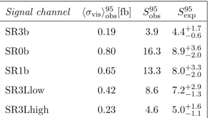
(21) 7.2.1. Gluino-mediated top squarks. Results for four simplified models of gluino-mediated top squark production are presented in figure 5. In each case, gluinos are produced in pairs, the top squark t̃1 is assumed to be (∗) the lightest squark, and the g̃ → tt̃1 branching fraction is set to 100%. The top squark, 0 χ̃0 however, decays to a different channel in each model: t̃1 → tχ̃1 , t̃1 → bχ̃± 1 , t̃1 → c 1 or t̃1 → bs, with a 100% branching fraction. 0 In the gluino-mediated top squark → tχ̃1 model, the mass of the top squark is set to mt̃1 = 2.5 TeV and the masses of all other squarks are much higher (they are assumed to be decoupled). Gluinos decay through mediation by an off-shell top squark to a pair of 0 top quarks and a stable neutralino, g̃ → tt̃∗1 → tt̄ χ̃1 . The final state is therefore g̃g̃ → 0 0 bbbb W W W W χ̃1 χ̃1 , with the constraint that mg̃ > 2mt + mχ̃01 . Results are interpreted in 0 the parameter space of the gluino and χ̃1 masses (see figure 5(a)). Gluino masses below 0 950 GeV are excluded at 95% CL, for any χ̃1 mass. The sensitivity is dominated by SR3b. χ̃± In the gluino-mediated top squark → bχ̃± 1 model, the top squark is on-shell, the 1 0 0 mass is set to 118 GeV, the χ̃1 mass set to 60 GeV and the χ̃1 is stable. Hence the chargino 0 0 decays through an off-shell W boson, and the final state is g̃g̃ → bbbb W W W ∗ W ∗ χ̃1 χ̃1 ,. with the constraint that mg̃ > mt + mt̃1 . Results are interpreted in the parameter space of the gluino and top squark masses (see figure 5(b)). Gluino masses below 1 TeV are excluded at 95% CL for top squark masses above 200 GeV. The sensitivity is dominated by SR3b. 0 In the gluino-mediated top squark → cχ̃1 model, the on-shell top squark and stable 0 neutralino have close-by masses, ∆m(t̃, χ̃1 ) = 20 GeV, which forbids the top squark decay to a top quark but allows the decay to a charm quark. The final state is therefore g̃g̃ → 0 0 bb cc W W χ̃1 χ̃1 , with the constraint that mg̃ > mt + mc + mχ̃01 . Results are interpreted in the parameter space of the gluino and top squark masses (see figure 5(c)). Gluino masses 0 below 640 GeV are excluded at 95% CL, for any t̃1 and χ̃1 masses. The sensitivity is dominated by SR1b. In the gluino-mediated top squark → bs (RPV) model, top squarks are assumed to decay with an R-parity-violating and baryon-number-violating coupling λ00323 = 1, as pro-. – 20 –. JHEP06(2014)035. SUSY theory line. The yellow band around the in this section are derived from the −1σtheory expected limit shows the ±1σ uncertainty, including all statistical and systematic uncertainties except the theoretical uncertainties on the SUSY cross section. The uncertainties on the SUSY signal include the detector simulation uncertainties described in section 6.2. For simplified models, 95% CL upper limits on cross sections obtained using the signal efficiency and acceptance specific to each model are available in the HepData database [74]. When available, exclusion limits set by previous ATLAS searches [75–79] are also shown for comparison. Three categories of simplified models are used to design the signal regions and interpret the results: gluino-mediated top squark, gluino-mediated (or direct) first- and second-generation squark, and direct bottom squark production, as illustrated in figure 1. In addition, three complete SUSY models and one mUED model are used for interpretation only..
(22) ~ 0 ~ g~ g production, ~ g→ tt∼ χ , m(t1) >> m(~ g). ~ ~ ~ 0 ± ± ~ g→ tt1, t1 → b∼ χ , m(t1) < m(~ g), m(∼ χ ) = 60 GeV, ∼ χ = 118 GeV. m~t [GeV]. 1. ATLAS 1200. ∫ L dt = 20.3 fb , -1. s=8 TeV. 2 same-charge leptons/3 leptons + jets. 1000. 1. ∫ L dt = 20.3 fb , -1. 1400. 1. s=8 TeV. 2 same-charge leptons/3 leptons + jets SUSY. SUSY. Observed limit (± 1 σtheory). Observed limit (± 1 σtheory) Expected limit (± 1 σexp) 0 lepton, >= 3 bjets, s= 7 TeV, 4.7 fb-1. 1200. Expected limit (± 1 σexp) 0 lepton, 7-10 jets, s=8 TeV, 20.3 fb-1 0 lepton, >= 3 bjets, s=7 TeV, 4.7 fb-1. 800. 1. ATLAS. 1600. 1. 1400. 1. mχ∼0 [GeV]. 1600. All limits at 95% CL. 1000. All limits at 95% CL. 800 600 ∼0. 400. 2*m. t. + mχ1. < mt. + m t1 ~. 400 200. 0. 600 700 800 900 1000 1100 1200 1300 1400 1500. 700. m~g [GeV]. 800. 900. 800. ~ 0 0 ~ g~ g production, ~ g→ tc+∼ χ , m(∼ χ ) = m(t1) - 20 GeV 1. 1. ATLAS. ∫ L dt = 20.3 fb , -1. s=8 TeV. ATLAS 900. ∫ L dt = 20.3 fb , -1. SUSY. Expected limit (± 1 σexp). 700. 400. < ~ mg. 300. + mt. +. All limits at 95% CL. 600. 0. mc. s=8 TeV. Observed limit (± 1 σtheory) Expected limit (± 1 σexp) 0 lepton, 7-10 jets, s=8 TeV, 20.3 fb-1. 800. All limits at 95% CL. 500. 1300. m~g [GeV]. 2 same-charge leptons/3 leptons + jets. Observed limit (± 1 σtheory). 700. 1200. ~ ~ ~ g~ g production, ~ g→ t1t, t1 (RPV)→ bs. 2 same-charge leptons/3 leptons + jets SUSY. 600. 1000. 1. 900. 1100. (b) m~t [GeV]. 1000. 1. m~t [GeV]. (a). 1000. m ∼χ 1. 500 400. 200 100. 300 400. 500. 600. 700. 800. 900. 1000 1100 1200. m~g [GeV]. (c). 200. 300. 400. 500. 600. 700. 800. 900 1000 1100. m~g [GeV]. (d). Figure 5. Observed and expected exclusion limits on gluino-mediated top squark production, √ obtained with 20.3 fb−1 of pp collisions at s=8 TeV, for four different top squark decay modes (see text). When available, results are compared with the limits obtained by previous ATLAS searches [78, 79].. posed in ref. [80]. The final state is therefore g̃g̃ → bbbb ss W W , characterised by the presence of four b-quarks but only moderate missing transverse momentum. Results are interpreted in the parameter space of the gluino and top squark masses (see figure 5(d)). Gluino masses below 850 GeV are excluded at 95% CL, almost independently of the top squark mass. The sensitivity is dominated by SR3b. Stringent limits are hence placed on gluino-mediated top squark scenarios favoured by naturalness arguments. The SR3b signal region is sensitive to almost any scenario with SS or ≥3 leptons and ≥3 b-quarks. This is demonstrated in the gluino-mediated top squark → bs (RPV) model, where mg̃ < 850 GeV is excluded by SR3b alone in the absence of a miss signature. In R-parity-conserving scenarios, the sensitivity is further increased large ET 0 by including the SR3Lhigh and SR1b signal regions. Results on gluino-mediated t̃1 → tχ̃1. – 21 –. JHEP06(2014)035. 200. < m~g. m~g. 600.
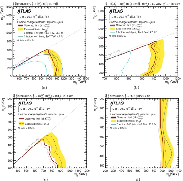
(23) and t̃1 → bχ̃± 1 show that mg̃ . 950 GeV is excluded for on-shell or off-shell top squarks, largely independently of the top squark mass, as long as the top squark decay involves 0 b-quarks. As shown for the gluino-mediated top squark → tχ̃1 model, this conclusion holds 0 0 for ∆m(g̃, χ̃1 ) ' 2mt as well. In the especially difficult gluino-mediated top squark → cχ̃1 case, where only two b-quarks and two W bosons are produced, gluino masses can still be excluded up to 840 GeV. 7.2.2. Gluino-mediated (or direct) first- and second-generation squarks. 0 0 g̃g̃ → qqq 0 q 0 W (∗) W (∗) χ̃1 χ̃1 ,. 0 0 q̃ q̃ → q 0 q 0 W ±(∗) W ∓(∗) χ̃1 χ̃1 .. The g̃g̃ model is the simplest strong-production scenario from which prompt same-sign leptons can arise, due to the Majorana nature of gluinos. However, the q̃ q̃ model can only produce opposite-sign leptons, for which this search has no sensitivity. Results are 0 interpreted in the parameter space of the gluino and χ̃1 masses (see figure 6(a)). This 0 scenario is excluded at 95% CL for gluino masses up to 860 GeV and χ̃1 masses up to 400 GeV. The sensitivity is dominated by SR0b. 0 In the gluino-mediated or direct squark → q 0 W Z χ̃1 model, squarks decay as 0. 0. 0 0 χ̃ χ̃ q̃ → q 0 χ̃± 1 → q W 2 → q W Z 1.. The intermediate particle masses are set to mχ̃± = (mg̃ + mχ̃01 )/2, 1. mχ̃02 = (mχ̃± + mχ̃01 )/2. 1. The final states are therefore 0 0 g̃g̃ → qqq 0 q 0 W (∗) W (∗) Z (∗) Z (∗) χ̃1 χ̃1 ,. 0 0 q̃ q̃ → q 0 q 0 W ±(∗) W ∓(∗) Z (∗) Z (∗) χ̃1 χ̃1 . 0. The W and Z bosons are on-shell (off-shell) at large (small) mass differences ∆m(g̃, χ̃1 ) 0 and ∆m(q̃, χ̃1 ). Results are interpreted in the parameter space of the gluino (squark) and. – 22 –. JHEP06(2014)035. Results for five simplified models of direct and gluino-mediated first- and second-generation squark production are presented in figure 6. In all models, the four squarks of first and second generations, collectively referred to as “squarks” (q̃), are assumed to be left-handed and degenerate in mass. These squarks are pair-produced, either directly (q̃ q̃) or via gluinos 0 (g̃g̃ → qq q̃ q̃), and the χ̃1 is assumed to be stable. Different assumptions on the decay of 0 0 the squarks are considered: q̃ → q 0 W χ̃1 , q̃ → q 0 W Z χ̃1 and q̃ → sleptons. The masses of the resulting supersymmetric particles are set according to commonly used conventions in order to cover a variety of scenarios. ± 0 0 In the gluino-mediated or direct squark → q 0 W χ̃1 model, the χ̃1 and χ̃1 masses are related by mχ̃± = 2mχ̃01 . For gluino-mediated and direct squark production, the final states 1 are therefore.
(24) 0 0 0 ± ~ g~ g → qqq'q'WW ∼ χ∼ χ , m(∼ χ ) = 2 m(∼ χ) 1 1. 1. 1. ATLAS. 1000. ∫ L dt = 20.3 fb , -1. 1. mχ∼0 [GeV]. 1100. 900. s=8 TeV. 2 same-charge leptons/3 leptons + jets SUSY. Observed limit (± 1 σtheory) Expected limit (± 1 σexp) 1 lepton, s=7 TeV, jets, 4.7fb-1 0 lepton, 7-10 jets, s=8 TeV, 20.3 fb-1 0-lepton, 2-6 jets, s= 7 TeV, 4.7 fb-1. 800 700 600. All limits at 95% CL. 500. 0. < m~g. m ∼χ 1. 400 300. 100. 400. 500. 600. 700. 800. 900. 1000 1100 1200. m~g [GeV]. (a) 1200. m∼χ0 [GeV]. 1 1. ATLAS. -1. 1000. s=8 TeV. 1000. 1. ∫ L dt = 20.3 fb ,. 1. mχ∼0 [GeV]. 0 0 ~ g~ g production, 2-step decay: ~ g~ g → qqq'q'WZWZ∼ χ∼ χ. 2 same-charge leptons/3 leptons + jets SUSY. ∫ L dt = 20.3 fb , -1. s=8 TeV. 2 same-charge leptons/3 leptons + jets SUSY. Observed limit (± 1 σtheory) Expected limit (± 1 σexp) 1 lepton, jets, s=7 TeV, 4.7fb-1 All limits at 95% CL. 600. < m∼χ 1 0. m~q. ∼χ0 1. 500. mg. 600. 900. 700. All limits at 95% CL. <m ~. 1 1. ATLAS. 800. Observed limit (± 1 σtheory) Expected limit (± 1 σexp) 0 lepton, 7-10 jets, s=8 TeV, 20.3 fb-1 1 lepton, jets, s=7 TeV, 4.7fb-1. 800. 0 0 ~ q~ q production, 2-step decay: ~ q~ q → q'q'WZWZ∼ χ∼ χ. 400 400. 300 200. 200 500. 600. 700. 800. 900. 1000. 1100. (b). 1200. 100 500. 1300. mg~ [GeV]. 1000. 1. m∼χ0 [GeV]. s=8 TeV. 2 same-charge leptons/3 leptons + jets. 700. 750. 800. 850. 900. mq~ [GeV]. 900. 1. 1. ATLAS. ∫ L dt = 20.3 fb , -1. s=8 TeV. 2 same-charge leptons/3 leptons + jets. SUSY. SUSY. Observed limit (± 1 σtheory). Observed limit (± 1 σtheory). 700. All limits at 95% CL. 600. Expected limit (± 1 σexp) All limits at 95% CL. 500. 600. 0. <. m ∼χ 1. 0. 400. ~ mg. 400. < m~q. m ∼χ 1. 300 200. 200 400. 650. 0 0 ~ q~ q decays via sleptons, ~ q~ q → q'q'll(ll)∼ χ ∼ χ + neutrinos. 800. Expected limit (± 1 σexp). 800. 1000. 1. ∫ L dt = 20.3 fb , -1. 1. mχ∼0 [GeV]. 1. ATLAS. 600. (c). 0 0 ~ g~ g decays via sleptons, ~ g~ g → qqq'q'll(ll)∼ χ ∼ χ + neutrinos. 1200. 550. 600. 800. (d). 1000. 1200. 100 300. 1400. mg~ [GeV]. 400. 500. 600. (e). 700. 800. 900. 1000. mq~ [GeV]. Figure 6. Observed and expected exclusion limits on gluino-mediated production of first- and second-generation squarks (left) and direct production of first- and second-generation squarks √ (right), obtained with 20.3 fb−1 of pp collisions at s=8 TeV, for three different squark decay cascades (see text). When available, results are compared with the limits obtained by previous ATLAS searches [75, 76, 79].. – 23 –. JHEP06(2014)035. 200.
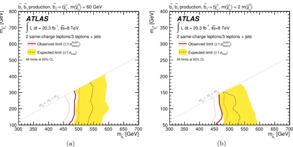
(25) ± ˜ → q 0 `ν χ̃01 , q̃ → q 0 χ̃1 → q 0 `ν ± 0 q̃ → q 0 χ̃1 → q 0 `ν̃ → q 0 `ν χ̃1 , 0 0 q̃ → q χ̃2 → q``˜ → q``χ̃1 , 0 0 q̃ → q χ̃2 → qν ν̃ → qνν χ̃1 .. Pair production of squarks or gluinos therefore leads to final states with missing transverse momentum, two or four light jets, and up to four charged leptons. Results are interpreted 0 in the parameter space of the gluino (squark) and χ̃1 masses (see figures 6(d) and 6(e)). These scenarios are excluded at 95% CL for gluino (squark) masses up to 1200 (780) GeV 0 and χ̃1 masses up to 660 (460) GeV. The sensitivity is dominated by SR3Lhigh. The signal regions SR0b, SR3Lhigh and SR3Llow are thus sensitive to first- and secondgeneration squark production in R-parity-conserving scenarios. The reach in gluino and χ̃01 masses varies by more than 300 GeV between the most difficult case (gluino-mediated 0 squark → q 0 W χ̃1 , with lowest leptonic branching fraction) and the most favourable case (gluino-mediated squark decaying via sleptons, with largest leptonic branching fraction). 0 In an intermediate case, the gluino-mediated squark → q 0 W Z χ̃1 model demonstrates the sensitivity of the SR3Lhigh signal region to signals involving on-shell Z bosons, which is an improvement compared to ref. [21]. Similarly, the limits on direct squark production are most stringent for long decay cascades involving sleptons, and less stringent for decays involving W and Z bosons because of the smaller leptonic branching fractions. However, none of the signal regions are sensitive to compressed first- and second-generation squark 0 0 scenarios with ∆m(g̃, χ̃1 ) or ∆m(q̃, χ̃1 ) smaller than ∼100 GeV. 7.2.3. Direct bottom squarks. Results for direct bottom squark production are shown in figure 7 for two simplified models. ± Both models assume bottom squark pair production, decaying as b̃1 → tχ̃1 , followed by ± 0 the chargino decay χ̃1 → W (∗)± χ̃1 , with branching fractions of 100%. In one model, the ± 0 neutralino mass is fixed to mχ̃01 = 60 GeV. In the other model, the χ̃1 and χ̃1 masses 0 are related by m ± = 2mχ̃0 . The χ̃1 is stable in both models. The final state is therefore b̃1 b̃1 → bb. χ̃1 W W W (∗) W (∗). 1. χ̃01 χ̃01 , with the constraint that m. – 24 –. b̃1. > mt + mχ̃± . In the fixed mχ̃01 1. JHEP06(2014)035. χ̃01 masses (see figures 6(b) and 6(c)). These scenarios are excluded at 95% CL for gluino 0 (squark) masses up to 1040 (670) GeV and χ̃1 masses up to 520 (300) GeV. The sensitivity 0 0 is dominated by SR3Lhigh at large ∆m(g̃, χ̃1 ) and ∆m(q̃, χ̃1 ) and by SR3Llow at small 0 0 ∆m(g̃, χ̃1 ) and ∆m(q̃, χ̃1 ). In the gluino-mediated or direct squark → sleptons model, squarks are assumed to ± ± 0 decay as q̃ → q 0 χ̃1 or q̃ → q χ̃2 with equal probability. The χ̃1 decays with equal ± 0 0 ˜ or χ̃± ˜ probability as χ̃1 → `ν 1 → `ν̃. The χ̃2 decays with equal probability as χ̃2 → `` or 0 0 0 χ̃2 → ν ν̃. Finally the slepton decays as `˜ → `χ̃1 , and the sneutrino decays as ν̃ → ν χ̃1 . All three flavours of sleptons are considered and are degenerate in mass. The masses of the 0 χ̃± 1 and χ̃2 are assumed to be equal and set to mχ̃± = mχ̃0 = (mg̃/q̃ + mχ̃0 )/2. The masses 2 1 1 of the slepton and sneutrino are assumed to be equal and set to m`˜ = mν̃ = (mχ̃02 +mχ̃01 )/2. The resulting decay chains are.
Figure

+7
Documento similar
51b High Energy Physics Institute, Tbilisi State University, Tbilisi, Georgia. 52 II Physikalisches Institut, Justus-Liebig-Universita¨t Giessen,
51b High Energy Physics Institute, Tbilisi State University, Tbilisi, Georgia. 52 II Physikalisches Institut, Justus-Liebig-Universit¨at Giessen,
50b High Energy Physics Institute, Tbilisi State University, Tbilisi, Georgia. 51 II Physikalisches Institut, Justus-Liebig-Universita¨t Giessen,
Andronikashvili Institute of Physics, Tbilisi State University, Tbilisi, Georgia 51b High Energy Physics Institute, Tbilisi State University, Tbilisi, Georgia 52 II
Javakhishvili Tbilisi State University, Tbilisi; b High Energy Physics Institute, Tbilisi State University, Tbilisi, Georgia 52 II Physikalisches Institut,
Javakhishvili Tbilisi State University, Tbilisi; b High Energy Physics Institute, Tbilisi State University, Tbilisi, Georgia 52 II Physikalisches Institut,
Javakhishvili Tbilisi State University, Tbilisi; b High Energy Physics Institute, Tbilisi State University, Tbilisi, Georgia 52 II Physikalisches Institut,
Javakhishvili Tbilisi State University, Tbilisi, Georgia 51b High Energy Physics Institute, Tbilisi State University, Tbilisi, Georgia 52 II Physikalisches
