Wind Farm Integration Through VSC HVDC

Texto completo

(1)Instituto Tecnológico y de Estudios Superiores de Monterrey Campus Monterrey School of Engineering and Sciences. Wind Farm Integration Through VSC-HVDC A thesis presented by Cristian Pool Linares Sánchez. Submitted to the School of Engineering and Sciences in partial fulfillment of the requirements for the degree of. Master of Science in Energetic Engineering. Monterrey, Nuevo León. December 4th , 2018.

(2)

(3)

(4) Dedication To my parents, José Luis and Cecilia, for helping me and supporting me every step of the way. To all my close friends, for being there when I needed them..

(5) Acknowledgements To Armando Llamas, for providing me with the necessary means and resources for the development of this thesis. For his time, guide, support, advice and for allowing me to learn from him. To Federico Viramontes and Luis Camargo for being members of the committee and dedicating time to reading this thesis. To Osvaldo Micheloud, for trusting in me and awarding me this scholarship..

(6) Wind Farm Integration Through VSC-HVDC by. Cristian Pool Linares Sánchez Abstract High Voltage Direct Current (HVDC) systems has been an alternative method of transmitting electric power from one location to another with some inherent advantages over AC transmission systems. The efficiency and rated power carrying capacity of direct current transmission lines highly depends on the converter used in transforming the current from one form to another (AC to DC and vice versa). A well-configured converter reduces harmonics, increases power transfer capabilities, and reliability in that it offers high tolerance to fault along the line. Different HVDC converter topologies have been proposed, built and utilized all over the world. The two dominant types are the line-commutated converter (LCC) and the voltage-source converter (VSC). This thesis is focused on explaining the basic concepts of HVDC Systems and their usefulness for the integration of renewable energy. With the improvement in VSC technology and the advantages which it offers over LCC, VSC is bound to grow, and gain more recognition and market share, especially with the large-scale renewable energy integration into traditional AC power grids going on worldwide. Wind energy also has matured to a level of development at which it is ready to become a generally accepted power generation technology. This thesis provides a state of the art in the area of electrical machines and power-electronic systems for high-power wind energy generation applications. Wind power is considered as the most promising renewable energy and has been under extensive development globally..

(7) List of Figures 1 2 3 4 5 6 7 8 9 10 11 12 13 14 15 16 17 18 19 20 21 22 23 24 25 26 27 28 29 30 31 32 33 34 35 36 37. Policy drivers for the energy supply of the future . . . . . . . . . Gotland link in Sweden . . . . . . . . . . . . . . . . . . . . . . . . Variation of costs with line length . . . . . . . . . . . . . . . . . . Power transfer capability vs. distance . . . . . . . . . . . . . . . . Types of HVDC links, retrieved from [4] . . . . . . . . . . . . . . . Applications of HVDC links . . . . . . . . . . . . . . . . . . . . . . LCC system schematics . . . . . . . . . . . . . . . . . . . . . . . . Thyristors . . . . . . . . . . . . . . . . . . . . . . . . . . . . . . . . Thyristor circuit with RL load . . . . . . . . . . . . . . . . . . . . Three-phase bridge thyristor converter . . . . . . . . . . . . . . . Waveforms for the three-phase bridge thyristor converter . . . . Three-phase bridge thyristor converter with interface inductance Voltage drop due to gate pulse delay . . . . . . . . . . . . . . . . Waveform variation with ↵ . . . . . . . . . . . . . . . . . . . . . . Converter equivalent circuit during commutation . . . . . . . . . Waveforms for the three-phase bridge thyristor converter with Lt 6= 0 . . . . . . . . . . . . . . . . . . . . . . . . . . . . . . . . . . DC voltage as a function of firing angle . . . . . . . . . . . . . . . Ixtepec-Yautepec LCC line . . . . . . . . . . . . . . . . . . . . . . Copainalá-Kantenáh VSC line . . . . . . . . . . . . . . . . . . . . Seri-Cucapah VSC line . . . . . . . . . . . . . . . . . . . . . . . . Esperanza-Mezquital-Villa Constitución VSC line . . . . . . . . . IGBT symbol . . . . . . . . . . . . . . . . . . . . . . . . . . . . . . IGBT with antiparalell diode . . . . . . . . . . . . . . . . . . . . . A monopolar VSC HVDC transmission system based on a twolevel converter . . . . . . . . . . . . . . . . . . . . . . . . . . . . . Three-phase, two-level voltage-source converter for HVDC . . . . Output phase voltages of the VSC . . . . . . . . . . . . . . . . . . Output line voltages of the VSC . . . . . . . . . . . . . . . . . . . Switching gate signals for 180° conduction . . . . . . . . . . . . Switching gate signals for 120° conduction . . . . . . . . . . . . Line and phase voltages for 120° conduction . . . . . . . . . . . Interconnection of two ideal voltage sources . . . . . . . . . . . . Phasor diagram of the system shown in Figure 31 . . . . . . . . Phasor diagram when providing active and reactive power to an AC system . . . . . . . . . . . . . . . . . . . . . . . . . . . . . . . . Converter modulation techniques . . . . . . . . . . . . . . . . . . Principles of PWM . . . . . . . . . . . . . . . . . . . . . . . . . . . The modulation index is in function of Ar and Ac . . . . . . . . . Carrier and reference waves being compared, PWM gate signals shown below the comparison . . . . . . . . . . . . . . . . . . . . .. ii. 2 8 9 10 11 13 14 16 16 17 18 19 19 20 21 22 23 25 26 27 28 30 30 31 35 36 37 38 40 40 41 42 43 44 46 46 47.

(8) 38 39 40 41 42 43 44 45 46 47 48 49 50 51 52 53 54 55 56 57 58 59 60 61 62 63 64 65 66 67 68 69 70 71 72 73 74 75 76 77 78 79 80. The a-axis and the q-axis are initially aligned, then the dq reference frame rotates at a speed !t . . . . . . . . . . . . . . . Equivalent abc and dq0 representations . . . . . . . . . . . . . No harmonics present . . . . . . . . . . . . . . . . . . . . . . . . Second harmonic present . . . . . . . . . . . . . . . . . . . . . . Third harmonic present . . . . . . . . . . . . . . . . . . . . . . . Fourth harmonic present . . . . . . . . . . . . . . . . . . . . . . Fifth harmonic present . . . . . . . . . . . . . . . . . . . . . . . Wind power generation capacity by country . . . . . . . . . . . Components of a wind turbine . . . . . . . . . . . . . . . . . . . Onshore Wind Farm . . . . . . . . . . . . . . . . . . . . . . . . . Offshore Wind Farm . . . . . . . . . . . . . . . . . . . . . . . . . Evolution of wind turbine size . . . . . . . . . . . . . . . . . . . Power characteristics of a wind turbine. . . . . . . . . . . . . . Types of wind energy conversion systems . . . . . . . . . . . . . Single line diagram of HVAC and HVDC interconnections . . . Transmission technology for different capacities and distances Potential sites for wind power in Mexico . . . . . . . . . . . . . Wint Turbine HVDC Link . . . . . . . . . . . . . . . . . . . . . . Simulink model courtesy of Hydro-Québec . . . . . . . . . . . . VSC1 control . . . . . . . . . . . . . . . . . . . . . . . . . . . . . PLL & measurements block . . . . . . . . . . . . . . . . . . . . . VDC regulator . . . . . . . . . . . . . . . . . . . . . . . . . . . . . . . Current regulator . . . . . . . . . . . . . . . . . . . . . . . . . . An example of a hybrid control system with feedforward and feedback . . . . . . . . . . . . . . . . . . . . . . . . . . . . . . . . Uabc generation block . . . . . . . . . . . . . . . . . . . . . . . . VSC2 Control . . . . . . . . . . . . . . . . . . . . . . . . . . . . . Power produced by the source in the HVDC link . . . . . . . . Fourier analysis line voltage at the AC side of the rectifier . . . Fourier analysis line current at the AC side of the rectifier . . Results of the rectifier Side of a 0.3 seconds run . . . . . . . . Fourier analysis line voltage at the AC side of the inverter . . . Fourier analysis line current at the AC side of the inverter . . Results of the inverter Side of a 0.3 seconds run . . . . . . . . Power produced by the source in the HVDC link . . . . . . . . Fourier analysis line voltage at the AC side of the rectifier . . . Fourier analysis line current at the AC side of the rectifier . . Results of the rectifier Side of a 0.3 seconds run . . . . . . . . Fourier analysis line voltage at the AC side of the inverter . . . Fourier analysis line current at the AC side of the inverter . . Results of the inverter Side of a 0.3 seconds run . . . . . . . . Power produced by the source in the HVDC link . . . . . . . . Fourier analysis line voltage at the AC side of the rectifier . . . Fourier analysis line current at the AC side of the rectifier . . iii. . . . . . . . . . . . . . . . . . . . . . . .. 49 49 50 50 50 50 50 53 54 55 55 56 58 59 61 62 65 66 68 70 70 71 72. . . . . . . . . . . . . . . . . . . . .. 72 73 74 76 77 78 79 81 82 83 84 85 86 87 89 90 91 92 93 94.

(9) 81 82 83 84 85. Results of the rectifier Side of a 0.3 seconds run . . . . . . Fourier analysis line voltage at the AC side of the inverter . Fourier analysis line current at the AC side of the inverter Results of the inverter Side of a 0.3 seconds run . . . . . . Model from scratch . . . . . . . . . . . . . . . . . . . . . . .. iv. . . . . .. . . . . .. . . . . .. 95 97 98 99 102.

(10) List of Tables 1 2 3 4 5. HVDC links between the United States and Mexico . . . . . . . . HVDC projects under consideration in PRODESEN . . . . . . . . Ixtepec-Yautepec LCC line components . . . . . . . . . . . . . . . Commutation states for a three-phase voltage source converter Comparison between 180°and 120°modulation . . . . . . . . . .. v. 23 24 24 39 41.

(11) Contents Abstract. i. List of Figures. ii. List of Tables. v. 1 Chapter 1: Introduction 1.1 Background . . . . . . . . . . 1.2 Motivation . . . . . . . . . . . 1.3 Thesis objective and context 1.4 Research questions . . . . . 1.5 Methodology . . . . . . . . .. . . . . .. . . . . .. . . . . .. . . . . .. . . . . .. . . . . .. . . . . .. . . . . .. . . . . .. . . . . .. . . . . .. 1 2 3 4 5 5. 2 Chapter 2: Principles of HVDC Systems 2.1 Evolution of HVDC systems . . . . . . . . . . . 2.2 Comparison of AC vs DC transmission . . . . . 2.2.1 Economics of power transmission . . . . 2.2.2 Technical performance . . . . . . . . . . 2.2.3 Reliability . . . . . . . . . . . . . . . . . . 2.3 Types of DC links . . . . . . . . . . . . . . . . . 2.4 Applications . . . . . . . . . . . . . . . . . . . . 2.5 Introduction to LCC HVDC . . . . . . . . . . . . 2.5.1 Line-commutated Converter . . . . . . . 2.5.2 Thyristors . . . . . . . . . . . . . . . . . . 2.5.3 Three-Phase Bridge Thyristor Converter 2.6 HVDC in Mexico . . . . . . . . . . . . . . . . . . 2.6.1 Ixtepec-Yautepec . . . . . . . . . . . . . . 2.6.2 Copainalá-Kantenáh . . . . . . . . . . . . 2.6.3 Seri-Cucapah . . . . . . . . . . . . . . . . 2.6.4 Esperanza-Mezquital-Villa Constitución. . . . . . . . . . . . . . . . .. . . . . . . . . . . . . . . . .. . . . . . . . . . . . . . . . .. . . . . . . . . . . . . . . . .. . . . . . . . . . . . . . . . .. . . . . . . . . . . . . . . . .. . . . . . . . . . . . . . . . .. . . . . . . . . . . . . . . . .. . . . . . . . . . . . . . . . .. . . . . . . . . . . . . . . . .. 6 6 8 8 9 11 11 12 14 14 15 17 23 24 25 26 27. 3 Chapter 3: VSC-HVDC Systems 3.1 IGBTs . . . . . . . . . . . . . . 3.2 VSC-HVDC converter stations 3.3 Voltage-source converter . . . 3.3.1 Two-level converter . . . 3.3.2 Power transfer . . . . . 3.3.3 Pulse width modulation 3.4 DQ0 reference frame . . . . . .. . . . . . . .. . . . . . . .. . . . . . . .. . . . . . . .. . . . . . . .. . . . . . . .. . . . . . . .. . . . . . . .. . . . . . . .. . . . . . . .. 29 29 30 33 34 41 43 48. . . . . .. . . . . .. . . . . . . .. . . . . .. . . . . . . .. . . . . .. . . . . . . .. . . . . .. . . . . . . .. . . . . .. . . . . . . .. . . . . .. . . . . . . .. . . . . .. . . . . . . .. . . . . .. . . . . . . .. . . . . .. . . . . . . .. . . . . . . ..

(12) 4 Chapter 4: Wind Power Fundamentals 4.1 Components of wind power systems . . . . . . . 4.2 Onshore and offshore wind farms . . . . . . . . 4.3 Evolution of wind turbines . . . . . . . . . . . . 4.4 Turbine power . . . . . . . . . . . . . . . . . . . 4.4.1 Wind turbine power characteristics . . . 4.4.2 Wind energy conversion systems (WECS) 4.5 HVDC and wind power . . . . . . . . . . . . . . 4.6 Wind energy in Mexico . . . . . . . . . . . . . .. . . . . . . . .. . . . . . . . .. . . . . . . . .. . . . . . . . .. . . . . . . . .. . . . . . . . .. . . . . . . . .. . . . . . . . .. 51 53 55 55 57 57 58 61 64. 5 Chapter 5: Case Studies 5.1 Rectifier control and operation . . . . . . . . . . . . . 5.1.1 PLL & measurements . . . . . . . . . . . . . . 5.1.2 DC voltage regulator . . . . . . . . . . . . . . . 5.1.3 Current regulator . . . . . . . . . . . . . . . . 5.1.4 Reference signal generator . . . . . . . . . . . 5.2 Inverter control and operation . . . . . . . . . . . . . 5.3 Results: Two 25 MW loads, VDC = 680 V . . . . . . . 5.3.1 Results: VSC Converter acting as a Rectifier . 5.3.2 Results: VSC Converter acting as an Inverter 5.4 Results: Two 25 MW, 15 Mvar loads, VDC = 680 V . . 5.4.1 Results: VSC Converter acting as a Rectifier . 5.4.2 Results: VSC Converter acting as an Inverter 5.5 Results: Two 25 MW, 15 Mvar loads, VDC = 1000 V . 5.5.1 Results: VSC Converter acting as a Rectifier . 5.5.2 Results: VSC Converter acting as an Inverter. . . . . . . . . . . . . . . .. . . . . . . . . . . . . . . .. . . . . . . . . . . . . . . .. . . . . . . . . . . . . . . .. . . . . . . . . . . . . . . .. . . . . . . . . . . . . . . .. . . . . . . . . . . . . . . .. 66 69 70 71 72 73 74 76 76 80 84 84 88 92 92 96. 6 Chapter 6: Conclusions & Future Work. . . . . . . . .. . . . . . . . .. 100. vii.

(13) Chapter 1: Introduction This thesis entitled ”Wind Farm Integration Using VSC Converters” is a research that addresses the concepts that make up the technology known worldwide as HVDC, and its impact and applications on current electrical systems. There is a special focus on wind power systems and how VSC converters are of special use for their integration to the electric grid. Chapter 1 serves as an introduction to the research developed in this thesis. First, some background information is presented and the motivation for the thesis is established, later the problem of the thesis is exposed, the research questions are stated and the methodology that was followed in this project is explained. Chapter 2 focuses on presenting the principles of HVDC transmission such as the origins and evolution of HVDC systems, a brief comparison of AC and DC transmission (in economics, technical performance and reliability), types of topologies of HVDC systems, applications of HVDC systems and an introduction to Line-Commutated Converter (LCC) HVDC technology. Chapter 3 presents the main focus of this thesis: Voltage-Source Converter (VSC) HVDC technology. Voltage-source converters (specifically two-level converters) are analyzed thoroughly, from the power electronic devices used (IGBTs) to the operation and power transfer of the converters. Sinusoidal Pulse Width Modulation (SPWM) is explained and the DQ0 reference frame is presented for control purposes. Chapter 4 centers on wind power fundamentals, with a special focus on the electric components of wind turbines and different topologies of wind energy conversion systems. The relationship of HVDC systems and wind power is also presented in this chapter. Chapter 5 presents a didactic Simulink model of a VSC-HVDC link. The components of this system are analyzed and the control strategy is meticulously explained. Finally, the results of some simulation scenarios 1.

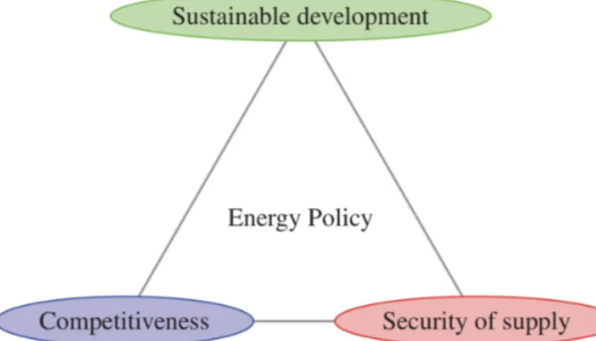
(14) are presented. Chapter 6 serves as a closure to this thesis, presenting the conclusions drawn across this work and stating some future work might the occasion to continue with this project arise. 1.1. Background. Although the priorities concerning energy policy differs between countries and regions, they are generally built around the same main pillars. Energy policy has the objective to ensure an energy provision that is reliable, costeffective, and sustainable. Given the importance of energy to the overall economy, a secure energy supply is crucial to the modern industry and society as a whole. The security of supply (SoS) requires the system to have sufficient resources available (adequacy), the infrastructure available to transmit the energy from the source to the consumer with sufficient redundancy, and the ability to deliver the energy at any given moment. Failure to do so leads to shortterm economic and national security concerns in the form of (local or widescale) blackouts. The relative economic position of a country or region can be compromised if the security of supply is threatened over a longer period of time. The second aspect is a cost-effective energy supply, which also has a direct impact on the economy of a country or region. A cost-effective energy supply. Figure 1: Policy drivers for the energy supply of the future 2.

(15) requires access to the cheapest energy sources. The last pillar of energy policy is a sustainable energy supply. Sustainable can be understood as an energy provision that can be maintained on a longer time horizon (e.g., using only sources that are non-exhaustible) or more narrowly as an energy provision that can be maintained over a longer time horizon considering the environment and society effects (e.g., using only renewable energy sources) [1]. Mexico’s National Electric System Development Program (PRODESEN) 2017-2031, published June 1, 2017 by Mexico’s Ministry of Energy (SENER) details a fifteen-year infrastructure development agenda that addressed important elements of the national electricity system, including all generation, transmission and distribution requirements [2]. By means of this program; the efficiency, quality, reliability and security of the National Electric System (SEN) is guaranteed by: • Diversifying the energy matrix, thereby ensuring Mexico’s energy security. • Installing enough resources to satisfy Mexico’s energy demands and comply with clean energy goals. • Installing the necessary infrastructure to correct functioning of the National Electric System. • Establishing an efficient generation expansion program that minimizes generation costs (by reducing congestion in transmission lines). 1.2. Motivation. The radical changes experienced by the transmission system in recent decades, along with the fast increase of renewable power generation (i.e. wind and solar) in the energy mix, have triggered the interest in HVDC (High Voltage Direct Current) grids. This has lead to a need to expand transmission capacity to integrate renewable technologies into the National Electric System. In order to do that, energy highways (long transmission lines) must be built due to the fact that most (if not all) renewable energy sources are located far away from load centers, and the existing transmission capacity 3.

(16) is severely limited. Furthermore, substations are not available at remote locations therefore increasing the costs of renewable energy projects. HVDC transmission systems promise to be a viable solution to the integration of renewable energy resources to the electric grid. Among the advantages of HVDC, we find that for long distances this type of systems is cheaper and has less electric losses than a traditional AC system [3]. This is due to the fact that a direct current system does not transmit reactive power (although converters might consume reactive power from the AC grid). This means all the transmission capacity of HVDC power lines is used to transmit active power, thereby relieving congestion problems. In Mexico’s case, PRODESEN 2017-2031 outlines six HVDC projects to be developed over the next fifteen years [2]. The most known of these project is the HVDC line Ixtepec, Oaxaca - Yautepec, Morelos; which will be the first HVDC transmission line constructed in Mexico. This power line will have a length of 1,2000 circuit kilometers and a capacity of 3,000 MW. Another important project is the interconnection of the state of Baja California Sur to the National Electric System by means of an underwater HVDC connection, this is to decrease the generation costs in the peninsula and increase the strength of the system. 1.3. Thesis objective and context. Throughout the world, a growing awareness concerning the environmental footprint of human activity is noticed. Especially greenhouse gases are considered problematic for contributing to global warming. As the generation of electricity from fossil fuels is an important contributor to CO2 emissions, these sources are increasingly replaced by renewables. Classical generation (fossil fuels and nuclear) will not disappear and completely be replaced by RES on a short time horizon, but the system will evolve towards a new generation mix, with the traditional generation not necessarily located at the same location as it is now. Where the generation originally was placed near the load center or near the source of primary energy, a shift is noticed towards the latter. The development of direct current transmission lines is a viable option to meet the objectives of the energy transition to clean energy. The development 4.

(17) in semiconductor devices has allowed the HVDC technology to become important and contribute a considerable increase in the efficiency of the transmission of electrical energy. This contributes considerably to the integration of remote renewable energy sources (as in the case of the Ixtepec wind resource) [4]. In the case of Mexico, this is evidenced in the National Electric System Development Program 2017-2031 published by the Ministry of Energy, where there are at least 6 HVDC projects in the planning phase [2]. The objectives of this thesis are to answer why HVDC is favorable over AC technologies for bulk power transmission, what are the key technologies and challenges for developing an HVDC systems, and how do VSC converters work and why are they so heavily sought for wind power integration to the electric grid. 1.4. Research questions. The following research questions were formulated: • When and why is HVDC favorable over AC technologies for power transmission? • What are the key technologies and challenges of HVDC transmission? • How do VSC converters work? • Why are VSC used in wind power integration to the grid? 1.5. Methodology. This thesis is mainly a research project so the first step is naturally a literature review on the topics of focus: HVDC, voltage-source converters, wind power conversion systems and the relationship of Wind Power and HVDC. The next step is the validation of the concepts by means of a computer simulation model. Finally the conclusions are drawn and future work is proposed.. 5.

(18) Chapter 2: Principles of HVDC Systems High-voltage direct current (HVDC) transmission has been used in power transmission systems for over 50 years. Its main applications are the interconnection of nonsynchronous networks, long-distance transport of electrical energy, and submarine and underground cable transmission. The most commonly used systems are based upon line commutated converter (LCC) HVDC, using thyristor-based valves. Voltage source converter (VSC) HVDC technology, which uses faster power electronic switches, is a recent development which is seen as a game changer and as the key enabling technology for future DC grids. In this section the basic concepts of HVDC transmission systems will be presented, including information on the evolution of this technology, technical information regarding the different configurations of the systems and the state of the art of the technology and of the semiconductor devices. Also, a brief introductions to HVDC projects in Mexico and some of their specifications will be presented. 2.1. Evolution of HVDC systems. Since the invention of the voltaic cell in 1799, the generation, transmission and distribution of electrical energy have evolved considerably. Although the first DC electric generator was created in 1832 by Hippolyte Pixii, the usefulness of electric power was evident until the creation of the vacuum glass bulb by Thomas Edison in 1879. As a result of Thomas Edison’s strong commitment to direct current, the main advances in accumulators and electric generators were made in this technology. For this reason, in 1882 a direct current line of 2 kV of 50 km was built between Miesbach and Munich in Germany. The first distribution networks installed in Europe and the USA worked in DC at low voltages, but much of the energy generated was lost in transmission.. 6.

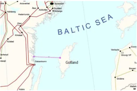
(19) The change from direct to alternating current came from the improvement of the AC generator, which allowed cheap and efficient electric energy generation by hydroelectric turbines. With the availability of transformers (for stepping up the voltage for transmission over long distances and for stepping down the voltage for safe use), the development of robust induction motor (to serve the users of rotary power), the availability of the superior synchronous generator, and the facilities of converting AC to DC when required, AC gradually replaced DC. In addition, the introduction of three-phase transmission in 1893 and advances in the construction of induction motors in the early twentieth century led to the use of alternating current as the only means of transmission of electrical energy [5]. The development of HVDC (High Voltage Direct Current) transmission system dates back to the 1930s when mercury arc rectifiers were invented. In 1941, the first HVDC transmission system contract for a commercial HVDC system was placed: 60 MW were to be supplied to the city of Berlin through an underground cable of 115 km in length. In 1945, this system was ready for operation. However, due to the end of World War II, the system was dismantled and never became operational [6]. Since the Second World War, and with the increase in energy needs, the interest of long distance links has increased. In 1950 a 116 km experimental link was built between Moscow and Kashira at a voltage of 200 kV. The first commercial HVDC system was built in Sweden in 1954, this consisted of a 98 km submarine power cable and a sea return to connect the island of Gotland with mainland Sweden. This transmission line was capable of transporting 20 MW of power at a voltage of 100 kV (up to 200 A of current). During the first twenty years there was a lot of experimenting with the stations on both sides of the cable, thus the Gotland link made a significant contribution to the development of HVDC as usable technology [7].. 7.

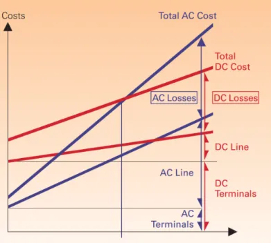
(20) Figure 2: Gotland link in Sweden. In the seventies, thanks to advances in power electronics, the first thyristor (solid state) valves were starting to be used in HVDC systems allowing the increased life and reliability of modern converters and reducing the costs of maintenance in a considerable way. By 2017, the line operating at the highest voltage and with the highest power transfer capacity is Xilingol League - Shandong in China (1000 kV and 9 GW respectively) [8]. 2.2. Comparison of AC vs DC transmission. The qualities of the two methods of transmission (AC and DC) that a system planner need to consider are: 1. Economics of transmission 2. Technical performance 3. Reliability 2.2.1. Economics of power transmission. The cost of a transmission line include the initial investment as well as the operational and maintenance costs. The initial investment include the Right of Way (a strip of land whose width depends on the voltage of the line and the height of the structures), the transmission towers, conductors, etc. Assuming similar characteristics for AC and DC conductors, it can be shown that a DC line can carry as much power with two conductors (with 8.

(21) Figure 3: Variation of costs with line length. positive and negative polarities with respect to ground) as an AC line with 3 conductors of the same size [9]. This means that for a given power level, DC lines require less RoW, simpler and cheaper towers and a reduced conductor cost. Power losses are also reduced as there are only two conductors. The other factors that influence the line costs are the costs of compensation and terminal equipment. DC lines do not require compensation but the terminal equipment costs are increased due to the presence of converters and filters. Figure 3 shows the variation of costs of transmission with distance for AC and DC transmission. For short distances, less than the break-even distance, AC tends to be more economical than DC (mostly due to the costs of the converters and the filters) [8]. As distances become bigger, AC losses and AC line costs become bigger making DC a more feasible. The break-even distance can vary from 500 to 800 km for overhead transmission lines, and be as little as 40 km for submarine transmission lines [1]. 2.2.2. Technical performance. DC transmission has some positive features when compared to AC transmission. These are mainly due to the controllability of power through. 9.

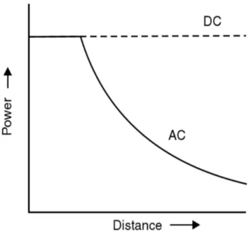
(22) Figure 4: Power transfer capability vs. distance. the converter stations. These advantages are: 1. Full control over power transmitted 2. The ability to enhance transient stability in associated AC networks 3. Fast control to limit fault current in DC lines make it feasible to avoid using expensive DC breakers in two terminal links. In AC lines, power transfer is dependant on the angle difference between the voltage phasors at the two ends [10]. For a given power level, this angle increases with the distance, therefore the maximum power transfer is limited by the considerations of steady state and transient stability of the system. For DC lines, the power carrying capability is unaffected by the distance of transmission and is limited only by the current carrying capacity of the conductors used (i.e. the thermal limit) [11]. The voltage control in AC lines also poses some complications caused by line charging and inductive voltage drops. The voltage profile in an AC line is flat only for a fixed level of power transfer corresponding to surge impedance loading1 [12]. The voltage profile varies with the line loading and requires shunt compensation at regular intervals (a serious problem in underwater 1 Surge impedance loading = The power delivered to a line by a purely resistive load equal to its surge impedance p Z0 = L/C. 10.

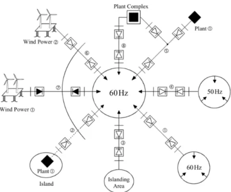
(23) cables) [1]. Also, the maintenance of constant voltages at the two ends requires reactive power control and the reactive power requirements increase with the increase in line lengths. 2.2.3. Reliability. An exhaustive record of HVDC links can be found in the literature from which statistics were computed and conclusions were drawn. The reliability of DC transmission systems is comparable to that of AC systems [13]. It must be pointed out that the performance of thyristor valves is much more reliable than mercury arc valves and further developments in power electronics are improving the reliability level of HVDC systems. The average failure rate of thyristors in valves is less than 0.6% per operating year. Also, it is common practice among manufacturers to provide redundant thyristors so that failed ones can be replaced during scheduled maintenance periods [9]. 2.3. Types of DC links. Figure 5: Types of HVDC links, retrieved from [4]. 11.

(24) 1. Monopolar links are mainly used for small systems. They have one conductor (usually of negative polarity) and use ground or sea return. If they are environmental restrictions, risk of corrosion or the terrain has a high electrical resistivity a metallic return is used [14]. 2. Bipolar links are the most common configuration. They have two conductors, one positive and the other negative. Each terminal has two sets of identical converters connected in series on the DC side [14]. The junction between the two sets of converters is grounded at one or both ends. Under normal operations, both piles operate at equal currents and, therefore, there is zero ground current flowing [15]. 3. Back-to-Back links consist of both converters (rectifier and inverter) operating under the same station. This configuration is usually used in asynchronous links between two AC systems where there is no need of DC transmission lines [16]. 4. A multi-terminal link consists of more than two converter stations connected by DC lines. A multi-terminal link could potentially enable the energy exchange between regions and facilitate the integration of solar and wind power to the electric grid, although their development has been halted mainly due to the need of HVDC breakers [17]. 2.4. Applications. HVDC transmission has been used in more than 150 point-to-point installations worldwide; in each case it has proven to be technologically and/or economically superior to AC transmission[14]. • Submarine power transmission: The AC cables have large capacitance and for cables over 40–70 km the reactive power circulation is unacceptable (although this distance can be extended somewhat with reactive power compensation). For larger distances, HVDC is more economical. A good example is the 580 km, 700 MW, 450 kV NorNed HVDC connection between Norway and the Netherlands.. 12.

(25) Figure 6: Applications of HVDC links. • Long-distance overhead lines: Long AC lines require variable reactive power compensation. Typically 600–800 km is the breakeven distance and, for larger distances, HVDC is more economical. A good example is the 1360 km, 3.1 GW, 500 kV Pacific DC Intertie along the west coast of the United States. • Interconnecting two AC networks of different frequencies: A good example is the 500 MW, 79 kV back-to-back Melo HVDC between Uruguay and Brazil. The Uruguay system operates at 50 Hz whereas Brazil’s national grid runs at 60 Hz. • Interconnecting two unsynchronized AC networks: If phase difference between two AC systems is large, they cannot be directly connected. A typical example is the 150 MW, 42 kV McNeill backto-back HVDC link between Alberta and Saskatchewan interconnecting asynchronous eastern and western American systems. • Controllable power exchange between two AC networks (for trading): The AC power flow is determined by the line impedances and it cannot therefore be controlled directly in each line. In complex AC 13.

(26) networks it is common to observe loop power flow or even overloading or underutilization of some AC lines. Many HVDC systems participate directly in trading power and one typical example is the 200 MW, 57 kV Highgate HVDC between Quebec and Vermont. 2.5 2.5.1. Introduction to LCC HVDC Line-commutated Converter. Thyristor-based high-voltage direct current transmission has been used in over 150 point-to-point installations all around the world. In each of this installations, it has been proven to be economically superior to AC transmission. A typical LCC system consists of two terminals and a DC line between them. Each terminal includes converters, transformers, filters, reactive power equipment, control station and other components. • Converters: They typically include one or more six-pulse thyristor bridges. Each bridge, often called a Graetz bridge, consists of six thyristor valves (which in turn contain hundreds of individual thyristors). In most systems, the bridges are connected in series in a 12-pulse or a 24-pulse configuration. • Converter Transformer: These transformers are designed to operate with. Figure 7: LCC system schematics 14.

(27) high harmonic currents and are designed to endure AC and DC voltage stress. • Smoothing Reactor: Typical inductances for large systems are in theorder of 0.1-0.5 H. • Reactive Power Compensation: The converters typically require reactive power of around 60% of the converter power rating. A large portion of this reactive power is supplied with filter banks and the remaining part with capacitor banks. Reactive power demand varies with DC power level, so the capacitors are arranged in switchable banks. • Filters: A typical 12-pulse thyristor terminal will require 11th, 13th, 23rd and 25th filters on the AC side. A high-pass filter is frequently included. In some cases third harmonic filters are required. Some HVDC systems with overhead lines also employ DC-side filters. • Electrodes: Some old HVDC systems normally operate with sea/ground return but most grid operators no longer allow permanent ground currents for environmental reasons. • Control and Communication System: Each terminal will have a control system consisting of several hierarchical layers. A dedicated communication link between terminals is needed but not critical, as an HVDC link can operate in the event of a loss of a communication link. 2.5.2. Thyristors. The thyristor, also known as the SCR (Silicone Controlled Rectifier), has been around since the mid-1950s. It is a four-layer (p-n-p-n), three-terminal device that can be considered as a controlled diode. When a reverse voltage (VAK < 0) is applied, the flow of current is blocked. When a forward voltage (VAK > 0) is applied, the current is blocked until a small positive voltage signal is applied to the gate with respect to the cathode. This small signal supplies a pulse gate current iG that sets the thyristor in its on state, and subsequently the gate-current pulse can be removed. The behavior of thyristors can be explained using a resistive circuit. At !t = 0, the voltage is positive and a forward voltage appears across the thyristor. If the device were a diode, a current would begin to flow into the circuit (this instant is called the instant of natural conduction). With the 15.

(28) Figure 8: Thyristors. thyristor, the start of conduction can be delayed with respect to the instant of natural conduction by an angle ↵, at which a gate-current pulse is applied. Once in the conducting state, the thyristor behaves just like a diode. As the current decline to zero at !t = ⇡, it cannot reverse through the thyristor and stays zero during the negative half-cycle, and until the gate pulse is applied in the next positive half-cycle. In most power circuits there are inductive elements, so their influence cannot be ignored most of the time. In Figure 9 the waveforms show that due to the inductor, the current comes to zero sometime during the negative half-cycle of the voltage. As in the resistive circuit, the current cannot reverse and remains zero for the remainder of the negative half-cycle, and until the gate pulse is applied in the next positive half-cycle.. Figure 9: Thyristor circuit with RL load. 16.

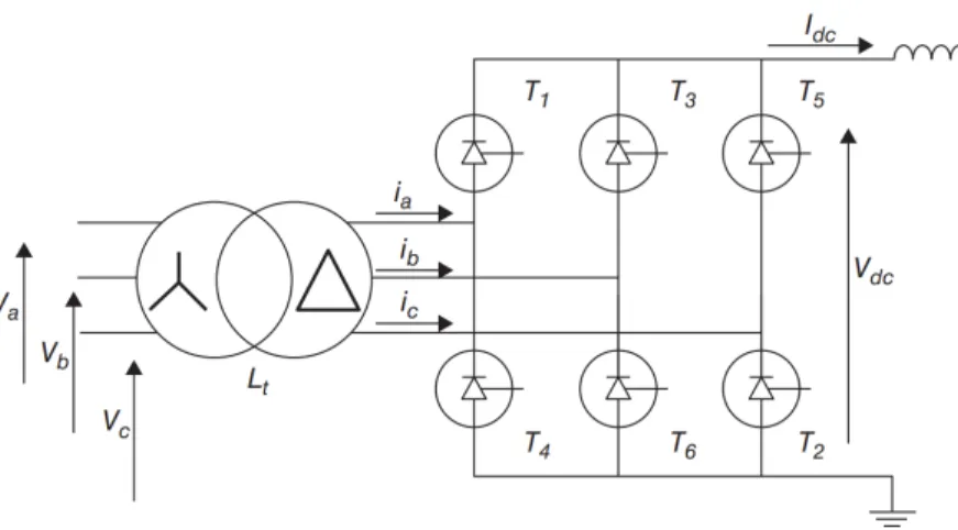
(29) 2.5.3. Three-Phase Bridge Thyristor Converter. To start the analysis of the three-phase thyristor converter it will be assumed that the thyristors are diodes (or that ↵ = 0). The AC system is assumed to be symmetrical and balanced, and the voltages are defined to be: ⇣ ⌘ va = V sin !t. ⇣ vb = V sin !t. 2 ⇡ 3. ⌘. (1). ⇣ ⌘ vc = V sin !t+ 23 ⇡. Where V is the magnitude of the phase voltage. Since ↵ = 0, the diodes will start conducting when they are forward-biased. Each diode conducts for 1/3 of the cycle (120°). At any given time, one diode conducts on the positive rail and one on the negative. In Figure 10 the arrangement of the six diodes in the converter can be seen. The positive rail are diodes D1, D3 and D5, while the negative rail are diodes D2, D6 and D4. Since they are six ”voltage pulses” (each lasting 60°), this converter is known as the six-pulse converter.. Figure 10: Three-phase bridge thyristor converter. The DC side inductor Ldc ensures that the DC currents stays approxi17.

(30) mately constant for the duration of one current pulse (120°). The diode bridge average DC voltage can be calculated by taking the average of the surface below vdc (t), to do this we can consider a 60°-segment in the six-pulse waveform, shown in Figure 11-b.. 1. Zb. f (x)dx. (2). p 3 2 2VLL cos !t d!t = VLL ⇡. (3). favg =. b. a. a. Vdc0. 3 = ⇡. Z⇡/6 p ⇡/6. By using thyristors and delaying the firing angle ↵, measured with respect to the instant of natural conduction, the average DC voltage can be regulated. By assuming the interface (or transformer) inductance Lt = 0, the commutation overlap is neglected and the converter waveforms are shown in Figure 13.. Figure 11: Waveforms for the three-phase bridge thyristor converter. 18.

(31) Figure 12: Three-phase bridge thyristor converter with interface inductance. The shaded area A↵ corresponds to a loss with units ”volt-radians” caused by delaying the gate pulse by ↵ every 60°.. Figure 13: Voltage drop due to gate pulse delay. The drop. V↵ can be calculated as: 3 V↵ = ⇡. Z↵ p. p 3 2 2VLL sin !t d!t = VLL 1 ⇡. cos ↵. (4). 0. Subtracting Equations 4 from Equation 3, the dc-side voltage can be found:. 19.

(32) p 3 2 Vdc↵ = VLL cos ↵ (5) ⇡ The behavior of Vdc↵ can be appreciated in the Figure 14, where alpha varies from ↵ = 0 to ↵ = 180°. As ↵ approaches 90° , the average DC voltage becomes zero. Beyond 90° the converter acts as an inverter, the power flow is reversed and the average DC voltage becomes negative.. Figure 14: Waveform variation with ↵. Since the interface inductance Lt 6= 0, we must consider its effect on the commutation from one thyristor to another. Typically the interface inductance is present within HVDC converters and the value of this inductance can be quite large, commonly in the order of 0.1–0.2 pu. Due to the presence of this inductance in the system, it takes a finite commutation interval µ for the current to commutate from one thyristor to the other. 20.

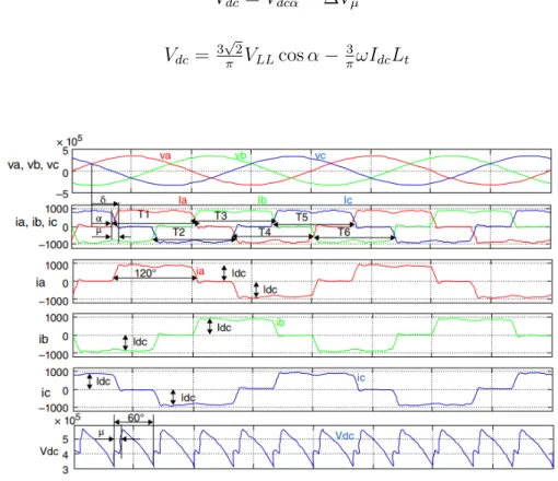
(33) During this interval µ, there is a commutating overlap, causing a DC voltage dip. To explain the mechanics of this overlap, an equivalent circuit will be used (shown in Figure 15). During the commutation overlap, three valves conduct simultaneously. The DC current is assumed to be constant, the current in phase a (and valve T1) gradually reduces, whereas the current in phase B (and valve T3) gradually increases.. Figure 15: Converter equivalent circuit during commutation. The commutation process has the effect of reducing the instantaneous b DC voltage to the value va +v . Due to the fact that the commutation process’s 2 duration depends on the direct current, the effect on the DC voltage similarly depends on the DC current of the system. The duration of the commutation process µ ( = ↵ + µ) can be found using the following equation: Idc 2!Lt p 2VLL. cos(↵ + µ) = cos(↵). The voltage drop due to commutation from one thyristor to another, can be calculated as: 3 Vµ = ⇡. Z. 3 vL d(!t) = !Lt ⇡. ↵. ZIdc. did =. 3 Idc !Lt ⇡. (6) Vµ ,. (7). 0. Where vL is the inductor voltage (vL = Lt · dis/dt) Therefore, considering the voltage drop due to delay in the gate pulse and 21.

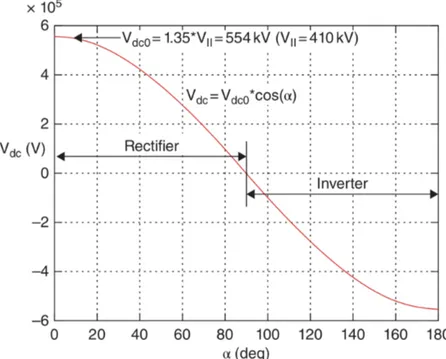
(34) the voltage drop due to the commutation process, the DC output voltage becomes: Vdc = Vdc↵ Vdc =. p 3 2 VLL ⇡. cos ↵. Vµ 3 !Idc Lt ⇡. (8). Figure 16: Waveforms for the three-phase bridge thyristor converter with Lt 6= 0. Figure 17 shows the converter DC voltage as a function of the firing angle. As the firing angle increases over 90°, the DC voltage becomes negative and the converter moves into inversion mode. Current cannot change direction in thyristor converters, so negative DC voltage implies power reversal.. 22.

(35) Figure 17: DC voltage as a function of firing angle. 2.6. HVDC in Mexico. As mentioned before, Direct Current Transmission Systems have been implemented in several parts of the world for quite some time, with more than 60 years of experience in LCC-based HVDC and almost 20 years in HVDC based on VSC. However, Mexico still does not have real HVDC systems. The existing HVDC links are two back-to-back facilities owned by American companies, both with the purpose of interconnecting with Mexico in an asynchronous manner. Both back-to-back converter stations were built by ABB Group. [18, 19] Name Eagle Pass Railroad DC Tie. Capacity 36 MW 300 MW. AC Voltage 132 kV 138 kV. DC Voltage 15.9 kV 21 kV. Technology Back-to-Back VSC Back-to-Back LCC. Table 1: HVDC links between the United States and Mexico. Although Mexico does not have HVDC facilities at the present time, there are several projects that are to be implemented in the coming years. In the National Electric System Development Program (PRODESEN), at least six HVDC link projects are mentioned. The HVDC projects that are expected to be in service for 2024 are shown on Table 2 [2, 20]. 23.

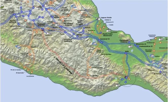
(36) 1 2 3 4 5 6. Project Ixtepec - Yautepec Seri - Cucapah Copainalá - Kantenáh Esperanza - Mezquital - Villa Constitución Nogales Back-to-Back Regiomontano - El Sauz. Capacity 3,000 MW 1,500 MW 1,500 MW 850 MW 150 MW 3,000 MW. DC Voltage 500 kV 500 kV 500 kV 400 kV 230 kV 500 kV. Technology LCC VSC VSC VSC LCC LCC. Table 2: HVDC projects under consideration in PRODESEN. Below, a description of the most advances projects outlined in PRODESEN will be presented. The first one expected to be built is the Ixtepec - Yautepec LCC line, which is already undergoing public bidding [21]. 2.6.1. Ixtepec-Yautepec. In 2015, SENER instructed CFE to carry out the direct current transmission line project Yautepec - Ixtepec. This new line will be able to transport up to 3,000 MW to vent the wind energy generated in the Isthmus of Tehuantepec and feed the Greater Mexico City metropolitan area. The project consists of the construction, modernization, operation and maintenance of 1,221 kilometers of electric transmission line circuits that will run at a voltage of 500 kV DC from Ixtepec, Oaxaca, to Yautepec, Morelos and two converter stations which will be line-commutated converters (LCC) [20]. The project has an investment of $1,200,000,000 USD and consists of 15 works spread across the states of Morelos, State of Mexico, Oaxaca, Mexico Ciy, Puebla and Veracruz. Figure 18 shows a schematic of the future DC transmission line and Table 3 show the works that compose the project [21]. Work 2. Converter Stations. 7. Electrical Substations. 5 1. AC Transmission Lines DC Transmission Line. Description Bipolar LCC at a voltage of ± 500 kV DC / 400 kV AC with a capacity of 3,000 MW / 7,200 MVA. At a voltage of 400 kV AC with a capacity of 1,750 MVA / 166.68 MVAr and 11 feeders. At a voltage of 400 kV and a total of 437.3 circuit kilometers. At a voltage of 500 kV and a total of 1,221 circuit kilometers.. Table 3: Ixtepec-Yautepec LCC line components. 24.

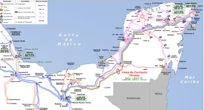
(37) Figure 18: Ixtepec-Yautepec LCC line 2.6.2. Copainalá-Kantenáh. The Yucatán peninsula is connected to the National Electric System by two 400 kV circuits and two 230 kV circuits. The evergrowing demand of electrical energy in the peninsula exceeds the national average mostly due to the development of tourism. The power generation of the peninsula is carried out through natural gas, fuel and diesel power plants, which recurrently present problems of unavailability. By the year 2022, problems are anticipated in the electrical energy supply, because the maximum predicted demand will exceed the limit of the transmission line between Valladolid and Cancún by 250 MW.. 25.

(38) Figure 19: Copainalá-Kantenáh VSC line. This project seeks the reduction of energy production costs in the Yucatán Peninsula and, at the same time, improve the reliability of the National Electric System. Since Copainalá is fed by hydroelectric power, this project will also help integrate cheap, clean, renewable power to the electric grid. The project has an investment of $1,142,000,000 USD, Figure 19 shows a schematic of the project. It consists of two VSC converter stations with a capacity of 1,800 MW each and a DC transmission line at a voltage of ±500 kV with a length of 1,800 circuit kilometers [20]. 2.6.3. Seri-Cucapah. This project will be the first HVSC line based on VSC technology. The link will allow the asynchronous interconnection of the electrical systems of Baja California to the National Electric System, through which great operational benefits are expected such as increasing flexibility, improving the stability of the system and the quality of the frequency and voltage [2]. The current plan will have an estimated investment of $1,100,000,000 USD and will consist of the interconnection of the Seri electrical substation in Sonora to the Cucapah electrical substation in Baja California by a DC link based con voltage source converters. The DC line will be 1,400 circuit 26.

(39) kilometers in a bipolar configuration [22].. Figure 20: Seri-Cucapah VSC line 2.6.4. Esperanza-Mezquital-Villa Constitución. Currently, Baja California Sur is composed of two systems that operate in isolation, Baja California Sur and Mulegé. The main load centers of Baja California Sur are located in the cities of La Paz, Cabo San Lucas and San José del Cabo, where tourism predominates. The Mulegé system supplies electricity to the north of the state, principally to the towns of Santa Rosalı́a, Guerrero Negro and Mulegé, where small populations with tourist activities predominate. The small size of the electricity grid in Baja California Sur makes it necessary to meet the demand with generation on base of small internal combustion units and gas turbine units, which consume fuel oil and diesel with high operating costs and a negative impact on the environment [2]. The proposed infrastructure will allow savings in investment costs in generation and transmission infrastructure, as well as in production costs for fuels and O&M. At the same time it will allow the integration of renewable generation and the full integration of the entire national electricity system. The project is expected to have an investment of $1,604,964,888 USD [23]. 27.

(40) The project consists of the construction of four DC line segments named: • Esperanza - Bahı́a de Kino • Bahı́a de Kino - El Infiernito • El Infiernito - Mezquital • Mezquital - Villa Constitución All of this lines will run at 400 kV in a bipolar configuration and, together, will have length of 1308 kilometers-circuit. Three voltage-source converter stations will located one at Esperanza, one at Mezquital and one at Villa Constitución; hence Esperanza-Mezquital-Villa Constitución will be the first multi-terminal HVDC system in Mexico [2].. Figure 21: Esperanza-Mezquital-Villa Constitución VSC line 28.

(41) Chapter 3: VSC-HVDC Systems The main shortcomings of LCC systems are large reactive power requirements (during both rectification and inversion), injection of low-order current harmonics and a dependency on a strong AC system to provide the commutating voltages (while risking commutation failures). These problems can be eliminated in self-commutating converters. Voltage source converter (VSC) systems are based on self-commutating switches, typically insulated-gate bipolar transistor (IGBT) technology, which have a number of advantages compared with thyristors. The use of selfcommutating devices allows the application of high-frequency (over 1 kHz) pulse-width modulation (PWM) techniques, which have been in use in the industrial drives sector since the early 1990s. By the use of PWM, the VSC may synthesize a fully controlled AC voltage, which enables precise control of active and reactive powers. This voltage appears as a fundamental frequency sine with harmonics at the switching frequency and its multiples. Because of higher switching frequencies, harmonics are lower and therefore filtering requirements are reduced. The use of VSCs for DC power transmission (VSC transmission) was introduced with the 3 MW, ±10 kV demonstrator at Hellsjön, Sweden in 1997. In this chapter VSC systems will be explained, the operation of the threephase VSC converter (both rectifier and inverter) will be analyzed and the use of pulse width modulation will be justified. 3.1. IGBTs. Although theoretically other semiconductor valves, such as MOSFETs or GTOs, could be used, all existing VSC-HVDC systems use voltage-driven IGBT (Insulated Gate Bipolar Transistor) technology. The history of IGBTs started in the early 1980s but major technological advances was made in 29.

(42) the 1990s when its feasibility for high-voltage applications was achieved and numerous companies started developing IGBT devices [15]. Insulated-gate bipolar transistors combine the advantages of Bipolar Junction Transistors (BJTs) and the Metal-Oxide Semiconductor Field-Effect Transistors (MOSFETs). IGBTs have high input impedance (low power characteristics) like the MOSFET with low conduction losses in the on-state like the BJT [24]. The IGBT is a voltage-controlled device that belongs to the transistor family. It can be switched on with a +15 V gate voltage and turned off when the gate voltage is zero. In practice, it is common to apply a negative voltage during the device-off operation to decrease any possible noise. Its fast switching speeds and near rectangular safe operating area allow the use of IGBTs without snubber circuits [25].. Figure 23: IGBT with antiparalell diode. Figure 22: IGBT symbol. The current capacity of an IGBT can be up to 6500 V, 2400 A and the commutation frequency can be in the order of 20 kHz (although losses increase with commutation frequency) [24]. 3.2. VSC-HVDC converter stations. The basic structure of a VSC-based HVDC system station is shown in Figure 24. The function and design of the major power components will be explained bellow:. 30.

(43) Figure 24: A monopolar VSC HVDC transmission system based on a two-level converter. AC Circuit Breaker The AC CB is employed to connect and disconnect the VSC HVDC system during normal and fault conditions. There are no special design requirements compared to normal AC CB used in power systems. VSC Converter Transformer A three-phase converter-grade transformer with tap-changer is use. The converter-side voltage is commonly controlled by the tap changer to achieve the maximum active and reactive power from the VSC, both consumed and generated. The converter transformer provides a coupling reactance between the VSC and the AC system, which also reduces fault currents and can decrease size of the AC filter. VSC Converter AC Harmonic Filters AC filters for VSC HVDC converters have lower ratings than those for LCC HVDC converters and are not required to provide reactive power compensation. A low-pass LC-filter is typically used to suppress highfrequency harmonic components. DC Capacitors The DC capacitor is the energy storage element in VSC. It provides the VSC with the stiff DC voltage between switching instants. A requirement for a small voltage ripple implies a large capacitor. On the other hand, a small capacitor has advantages considering the control and dynamics of the converter, which results in fast active power control. Selecting the size of the DC capacitor is a tradeoff between voltage ripple, lifetime, costs and the fast control of the DC voltage. Commonly, the high-power converter capacitor size is determined considering the total energy stored. The energy-to-power ratio Es [J/V A] is defined 31.

(44) using capacitor energy Ec [J] and the converter power SV SC [V A]: Es =. Ec SV SC. (9). The energy to power ratio in practical converters is: 10 (kJ/M V A) < Es < 50 (kJ/M V A), which is a good tradeoff between harmonic penetration and control performance. Using the expression for capacitor energy: 1 Ec = Cdc Vdc2 2 it is possible to obtain a formula for capacitor size: Cdc =. 2SV SC Es Vdc2. (10). (11). DC Filters Instead of increasing the size of the DC capacitor, a DC filter can be used to eliminate the targeted harmonics, which may be injected into the DC line. VSC HVDC Valves A valve in VSC HVDC converter requires numerous series connected cells to achieve the required blocking voltage. Several redundant cells are typically provided in each valve chain which ensure that voltage stress is within acceptable range even when a single (or few) cells fail. AC Reactors AC reactors are commonly added in series with VSC converter transformers on the converter side. They increase series reactance where it would be difficult to achieve such large transformer leakage inductance. The main purpose of AC reactors are to reduce DC fault currents and reduce peak switch currents for AC faults. DC Reactors In VSC HVDC systems, a DC reactor may be connected after the DC capacitor. They are used in order to reduce harmonic current in the DC overhead line or cable. A DC reactor in a VSC HVDC system is considerably smaller than those used in LCC HVDC and typically it is below 5 mH. Compared to the traditional LCC-HVDC system, the VSC-HVDC system is significantly smaller. This is due to the reactive power compensators and AC filters that are required in the LCC arrangement which are more voluminous 32.

(45) compared to the VSC solution, resulting in a significantly smaller footprint. 3.3. Voltage-source converter. Recent developments of power electronic devices have led to the rise of self-commutated voltage source converters (i.e. VSC) in power system applications. This is mainly attributed to the development of the IGBT, a device which combines the controllability of the MOSFET with the reliability and power rating of the BJT. VSC-HVDC transmission systems are experiencing great development. The first commercial VSC-HVDC system was commissioned in 1997 on the island of Gotland, Sweden. Since then, ratings and applications have progressed rapidly. The power and voltage for Gotland Light (manufactured by ABB) was 50 MW and ± 80 kV. Fifteen years later, power and voltage ratings have increased by a factor of 20 and 6 times, respectively. The full controllability allows the device to regulate power flow much more quickly. This technology also has the ability to absorb and generate both active and reactive power independently of one another. This eliminates the requirement for the expensive reactive power compensators, used extensively within LCC-HVDC systems. Further advantages are that there is no requirement for regulation of the short-circuit level as commutation can operate without an AC system voltage source. Also, the generation of harmonics is greatly reduced, minimizing the volume of filters required to absorb them. Additionally, voltage-source converters have the capability to offer “blackstart” support; that is, restoring power without the aid of an external power source. This is advantageous in big power outages as these power sources can be brought online first to begin the progressive restoration of the network grid. The main advantage of VSC converters, compared with line-commutated converters (LCCs) are: • Active and reactive power can be controlled independently. The VSC is capable of generating leading or lagging reactive power, independently of the active power level. • If there is no transmission of active power, both converter stations 33.

(46) operate as static synchronous compensators (STATCOMs) to regulate local AC network voltages. • The use of PWM with a switching frequency in the range of 1–2 kHz is sufficient to suppress the harmonic components around and beyond the switching frequency components. Harmonic filters are at higher frequencies and therefore have low size, losses and costs. • Power flow can be reversed instantaneously (50–100 ms) without the need to reverse the DC voltage polarity (only DC current direction reverses). • Black-start capability, which is the ability to start or restore power to a dead AC network (network without generation units). This feature eliminates the need for a generator in applications where space is critical or expensive, such as with offshore wind farms. The main limitations or disadvantages of VSC converters are: • Improved control is achieved at the expense of increased losses in the power converter. Increased losses are the result of: – Application of high frequency switching leads to increased switching loss. – IGBT devices exhibit significantly higher on-state voltage drop compared to thyristors of similar voltage ratings. • Higher costs than LCC converters. A VSC requires a larger number of semiconductors and the number of switches is much higher than with an LCC. • DC-side faults are a serious issue because a VSC behaves like an uncontrolled diode bridge during a DC fault. 3.3.1. Two-level converter. Most VSC-HVDC systems in operation right now are based on the two level converter. The two-level converter is the simplest type of three-phase voltage-source converter and can be thought of as a six pulse bridge in which the thyristors have been replaced by IGBTs with inverse-parallel diodes, and the DC smoothing reactors have been replaced by DC smoothing capacitors. An example of a two-level converter is shown in Figure 25. 34.

(47) These converters are called two-level converters since the voltage at the AC output of each phase is switched between two discrete voltage levels, corresponding to the electrical potentials of the positive and negative DC terminals. When the upper of the two valves in a phase is turned on, the AC output terminal is connected to the positive DC terminal, resulting in an output phase voltage of +1/2 Ud with respect to the midpoint potential of the converter. When the lower valve in a phase is turned on, the AC output terminal is connected to the negative DC terminal, resulting in an output phase voltage of 1/2 Ud. The simplest (and also, the highest-amplitude) waveform that can be produced by a two-level converter is a square wave. This, however, produces unacceptable levels of harmonic distortion and in practice needs to be reduced by using PWM. As a result of pulse-width modulation, IGBTs are switched on and off many times in each mains cycle. This results in high switching losses in the IGBTs and reduces the overall transmission efficiency.. Figure 25: Three-phase, two-level voltage-source converter for HVDC. A VSC based HVDC converter is similar to a STATic COMpensator (STATCOM). For the analysis of the three phase VSC the following assumptions were made: 1. The supply voltages are sinusoidal and balanced. 2. The switches are assumed to be ideal (that is losses are ignored). 3. The inductance L and resistance R are the parameters of the series reactor connected between the supply and the VSC (that represents the 35.

(48) leakage reactance and ohmic losses of the interfacing transformer). G represents the losses in the DC capacitor. The output phase voltages of the VSC are shown in the next figure:. Figure 26: Output phase voltages of the VSC. This voltages are related as: van (!t) = vbn (!t + 120°) = vcn (!t + 240°). (12). The relation between the line and phase voltages are: vab (t) = van. vbn. vbc (t) = vvn. vcn. vca (t) = vcn. van. 36. (13).

(49) These line voltages are presented below:. Figure 27: Output line voltages of the VSC. The instantaneous line voltages can be expressed using the Fourier series as follows: vab =. ⇣ n⇡ ⌘ ⇣ ⇣ 4Vdc ⇡ ⌘⌘ cos sin n !t + n⇡ 6 6 n=1,3,5,.... (14). vbc =. ⇣ n⇡ ⌘ ⇣ ⇣ 4Vdc cos sin n !t n⇡ 6 n=1,3,5,.... ⇡ ⌘⌘ 2. (15). ⇣ n⇡ ⌘ ⇣ ⇣ 4Vdc = cos sin n !t n⇡ 6 n=1,3,5,.... 7⇡ ⌘⌘ 6. (16). vca. 1 X. 1 X. 1 X. It should be noted that the triplen harmonics (odd multiples of three) will be zero in the line voltages.. 37.

(50) From Equation 14, the RMS value of the line voltages can be calculated as follows:. Vab =. s. 2 2⇡. Z. 2⇡/3. Vdc d!t = 0. r. 2 Vdc = 0.8165Vdc 3. (17). For n = 1, the line RMS fundamental voltage is: Vab1 =. 4Vdc cos (30°) p = 0.7797Vdc 2⇡. (18). For this type of operation, the conduction angle of each switch is 180° conduction, which is made in such a way that the two switches on the same converter leg do not conduct simultaneously (to prevent DC short circuit). The gate signal pulses needed to obtain these voltages are shown in Figure 28.. Figure 28: Switching gate signals for 180° conduction. The states of the converter are shown in Table 4, as it can be seen the line voltages switch between three discreet voltage levels Vdc , 0 and -Vdc .. 38.

(51) S1 , S2 , S1 , S3 , S1 , S4 , S2 , S1 , S3 , S1 , S4 , S1 ,. S5 S3 S2 S4 S2 S5 S3 S5 S4 S2 S5 S2. State and S6 open and and S4 closed and S6 open and and S5 closed and S3 open and and S6 closed and S4 open and and S6 closed and S5 open and and S6 closed and S6 open and and S3 closed. Number. Commutation State. vab. vbc. vca. 1. 101. Vdc. -Vdc. 0. 2. 100. Vdc. 0. -Vdc. 3. 110. 0. Vdc. -Vdc. 4. 010. -Vdc. Vdc. 0. 5. 011. -Vdc. 0. Vdc. 6. 001. 0. -Vdc. Vdc. Table 4: Commutation states for a three-phase voltage source converter. The frequency of the AC voltage can be controlled by changing the period of these gate signals, and the phase shift of the AC voltage can be controlled by varying the phase displacement of these signals (with the help of a phaselock loop to provide a reference phase). Another modulation technique used is 120° conduction. With this modulation technique the switches are fired for 120° (instead of 180°). As a result, at any instant, only two switches conduct. A dead time of 60° exists between two switches on the same converter leg (phase), resulting in a lower device use and lower RMS AC voltage than with 180° conduction. Both techniques give the same harmonic spectrum but 180° conduction gives 15% increase in AC voltage magnitude compared to 120° conduction. Figures 29-30 show the gate signal pulses and the line and phase voltage output waveforms for 120° conduction and Table 5 shows a comparison between both modulation techniques.. 39.

(52) Figure 29: Switching gate signals for 120° conduction. Figure 30: Line and phase voltages for 120° conduction. 40.

(53) Conduction technique 180°. Fundamental Voltage Peak RMS. Phase voltage. 2 ⇡ Vdc = 0.637Vdc p 2 3 ⇡ Vdc = 1.1Vdc. Line voltage 120°. Peak p. Phase voltage. 3 ⇡ Vdc. Line voltage. 3 ⇡ Vdc. = 0.551Vdc. = 0.955Vdc. p. 2 ⇡ Vdc p 6 ⇡ Vdc. = 0.45Vdc = 0.78Vdc. RMS p. 6 2⇡ Vdc. = 0.39Vdc. p3 Vdc 2⇡. = 0.39Vdc. Waveform characteristic Total RMS THD q p. 2. 3 q. = 0.471Vdc. 2 3 Vdc. = 0.816Vdc Total RMS p1 Vdc 6 p1 Vdc 2. = 0.408Vdc = 0.707Vdc. Table 5: Comparison between 180°and 120°modulation. q. ⇡2 9. 1 = 0.311. ⇡2 9. 1 = 0.311. ⇡2 9. 1 = 0.311. ⇡2. 1 = 0.311. THD q q. 9. Several different PWM strategies have been developed, but in all cases the efficiency of the two-level converter is significantly poorer than that of a LCC because of the higher switching losses. A typical LCC HVDC converter station has power losses of around 0.7% at full load (per end, excluding the HVDC line or cable) while with 2-level voltage-source converters it is 2-3% per end. Since the conduction in IGBTs is unidirectional, anti-parallel diodes are connected across them to ensure the bridge voltage has only one polarity (while current flows in both directions). 3.3.2. Power transfer. Power transfer can be explained by using the diagram in Figure 31, the figure shows an inductive line between two ideal voltage sources V1 and V2 (that can represent actual generators, voltage-source converts or nodes of an electric system).. Figure 31: Interconnection of two ideal voltage sources. The phasor diagram in Figure 32 represents the operating conditions of the interconnection between the voltage sources. Using V2 as a reference, the following expressions can be derived:. 41.

(54) Figure 32: Phasor diagram of the system shown in Figure 31. I2 X cos ( ) = V1 sin ( ) (19) I2 X sin ( ) = V1 cos ( ). V2. Since the active power entering node two is P = V2 I2 cos ( ) and the reactive power entering node 2 is is Q = V2 I2 sin ( ), the following expressions can be obtained: P = V2 I2 cos ( ) =. Q = V2 I2 sin ( ) =. V1 V2 sin ( ) X. V2 (V1 sin ( ) X. (20) V2 ). This has the implication that, in order to control P and/or Q it is necessary to vary one or more of the four variables V1 , V2 , and X. In practice, generator controls are slow and inefficient, and the power angle must be kept low in order to preserve transmission stability. When the voltage-source converter is connected to a passive network on the AC side, the power flows only in one direction (from the DC input side to the passive AC load). If the voltage-source converter is connected to an active AC system, the power can be made to flow in either direction by making the phase angle of the converter AC output voltage positive or negative with respect to that of the AC system voltage. The IGBTs must provide a unidirectional voltage on the DC side but need 42.

(55) Figure 33: Phasor diagram when providing active and reactive power to an AC system. to be able to conduct current in either direction if bidirectional power is expected. Figure 33 shows the phasors of the fundamental components of the AC ouput voltage and the AC system voltage. In this case the converter is acting as an inverter and supplying power (both active and reactive) to the AC system. 3.3.3. Pulse width modulation. The simple two-level converters have very little control capability. AC voltage magnitude control using converter modulation techniques has been the subject of intensive research during the last few decades. A large variety of methods have been developed and implemented. Their implementation in converters depends on the application type, the power level, the semiconductor devices and the harmonic level requirements. It is commonly performance and cost criteria that determine the choice of a modulation method in a specific application. Pulse-width modulated (PWM) voltage source inverters represent the dominant technology in use by the industry today and they are used widely in voltage source converter (VSC) high-voltage direct current (HVDC) systems. As shown in Figure 34 the modulation techniques can be classified as:. 43.

(56) • Six-pulse mode: Can be either 180° or 120 ° conduction. • Pulse-width modulation: Used with a two or three-level HVDC converters and with some modular multilevel HVDC converters (MMC). • Stepping: Used with some low-power, variable speed drives but not with HVDC.. Figure 34: Converter modulation techniques. A control of the output voltage is often needed in many industrial applications, the most efficient method for controlling the gain of a converter is by pulse width modulation. In general, several pulses are produced in each half cycle of the output voltage to reduce the harmonic content and to increase the harmonic frequencies (thereby reducing the cost and size of filters). PWM was originally designed around the needs of inverter-fed AC drives, as these require fast and continuous control of the frequency and voltage magnitude. Although such high level of controllability is not required in power transmission, where the frequency and voltage magnitude are only permitted to vary within narrow limits, the PWM concept has so far been adopted as the basis of a more flexible HVDC technology. An additional 44.

(57) benefit of the absence of passive filters for the low-order harmonics is the prevention of the converter/system harmonic interaction experienced by LCC systems. However, to be of practical use in power transmission the following two conditions must be met: 1. The output waveform should be free from even harmonics (either the phase waveforms possess half-cycle symmetry or any asymmetry is eliminated in the phase-to-phase voltages). Under this condition the phase-to-phase voltage will contain only odd-harmonic orders other than those multiples of three. 2. The three-phase system should be symmetrical; that is, the potentials of the three phases must have the same waveform but be displaced by 120° from each other. The generation of gate signals (in order to turn on or off the transistors) is achieved by comparing a reference signal with a triangular carrier wave. The frequency fr of the reference signal establishes the output frequency, while the ratio of the carrier signal’s frequency to the reference signal’s frequency mf = fc/fr. (21). determines the harmonic spectrum. A sufficiently large value of this ratio will reduce all the low-order harmonics to be within the specified limits. However, a high-frequency ratio will cause high switching losses. Also, the voltage–time area will be reduced and with it the fundamental component at full output voltage. When desired output of an inverter is a sine wave, a sinusoid is used as a reference signal (this technique of PWM is called sinusoidal PWM or SPWM). This has the effect of making the pulses vary in proportion with the amplitude of the sine wave; and causes the DF2 and the LOH3 to be reduced considerably. The control signals are achieved by comparing a sinusoid reference signal with a triangular carrier wave at a frequency fc . The amplitude of the reference sinusoid determines the modulation index and, therefore, the output voltage V0 . 2 Distortion 3 Lowest. factor order harmonic. 45.

(58) Figure 35: Principles of PWM. Ar (22) Ac where Ar is the amplitude of the reference signal and Ac is the amplitude of the triangular carrier wave. M=. Figure 36: The modulation index is in function of Ar and Ac. The same carrier wave can for all three phases with reference voltages shifted 120°. The ratio of the carrier signal’s frequency to the reference signal’s frequency mf should be an odd multiple of three, this way harmonics (which are due to the PWM process) will appear at: n = jmf ± k 46. (23).

(59) Figure 37: Carrier and reference waves being compared, PWM gate signals shown below the comparison. where j = 1, 3, 5... for k = 2, 4, 6 . . . and j = 2, 4 . . . for k = 1, 3, 5 . . . in a fashion that n is never a multiple of three (harmonics will appear in mf ± 2, mf ± 4, . . . ,2mf ± 1, 2mf ± 5, . . . , 3mf ± 2, 3mf ± 4 ,. . . , 4mf ± 1, 4mf ± 5, . . . ). The maximum amplitude of the fundamental component of the phase voltage in the linear region (that is 0 < M  1) is Vs/2 and the maximum p amplitude of the fundamental component of the line voltage is v̂ab1 = 3Vs/2. Therefore we can write the peak amplitude of the line voltages as: p Vs v̂ab1 = M 3 for 0 < M  1 2. (24). From the operational viewpoint the use of PWM adds considerable flexibility to the VSC. The modulation process develops independent fundamental and harmonic frequency voltage control from a constant DC source; this in turn provides four-quadrant power controllability and avoids the use of low-order harmonic filters. From the design viewpoint, however, the frequent and rapid switching of the AC bus voltage between two levels results in repetitive, high-frequency transient stresses, which affects the design of the VSC components and. 47.