Public university in Argentina: subsidizing the rich?

Texto completo

(1)Public University in Argentina: Subsidizing the Rich? Martín González Rozada a, Alicia Menéndez b ∗ a b. Cedes, Sánchez de Bustamante 27, Buenos Aires, Argentina Princeton University, Princeton, NJ, USA. Abstract. We analyze some characteristics of the higher education system in Argentina regarding equity and efficiency. Individuals attending the university belong to the top deciles of the income distribution and to relatively highly educated families. Almost 90 percent of the students in tuition-free public universities have higher than median per capita family income and almost 50 percent attended tuition-financed private high schools. We compare these students with those who attend non tuition-free private colleges. Although students in private universities seem to have higher per capita family income, this difference is not large enough to distinguish the two groups after controlling for other variables. These facts imply that there is an implicit transfer to the richest individuals in the society. We argue that equity and efficiency of the system can be improved by charging tuition-fees. Complementary, selective scholarships and loans could be offered to attract the most talented students from poor families.. Key words: University education, tuition fees, subsidy, equity JEL Classification: I2, H52. ∗. Corresponding author. 343 Wallace Hall, Woodrow Wilson School, Princeton University, Princeton, NJ 08544, USA. Email: [email protected]..

(2) 2. 1. Introduction In Argentina, like in most Latin American countries, the government heavily subsidizes higher education. The subsidy comes in the form of the central government financing tuition-free public universities and it is enjoyed by all students regardless their economic and academic background. Enrollment in those universities is open to all individuals with the only requirement of having a high school degree. In 1998, almost 83 percent of the more than one million undergraduates in the Greater Buenos Aires area were students at public universities1. During the last decade, this figure has been increasing at an average annual rate of approximately 3.6 percent. One of the most important implications of this is the overpopulation in public institutions with an associated decrease in the quality of education. The current organization of the provision of public higher education presents several other problems. Among them, the most obvious is the availability of public funds for a growing number of students given the severe fiscal restrictions of the country. This increasing scarcity of public funds is not only due to macroeconomic conditions but also due to the competition for these funds from other public needs such as basic education, health care, poverty reduction programs, public infrastructure, etc. The system has also distributional consequences. Standard models of public provision of college education, for example, tend to imply a transfer from the rich to the poor, however, empirical studies (Psacharopoulos et al., 1986) and new theoretical work (Fernandez and Rogerson, 1995) show that free higher education implies a transfer from lower income groups to higher income groups. Other problems related to the tuition-free system are the low rate of graduation among students and the excessive number of years they take to complete their college studies. Official figures show that, on average, in 1995 for each one hundred new. 1. Secretaría de Políticas Universitarias, “ Módulo Especial de Educación, Encuesta Permanente de Hogares, Mayo 1998”.

(3) 3. students that enrolled in public universities, only 19 students graduated2. In general, students spend many more years to finish their college education than they should. The average student takes 60 percent more time to complete her university studies than the theoretical duration indicates. Both numbers clearly indicate a waste of resources that would be likely to be reduced by increasing academic performance requirements and the pecuniary cost of being a public university student. Students attending public universities defend, of course, the status quo. They are active, organized, and very vocal. The defense of the tuition-free university is made on the grounds of equal opportunity and access to higher education for all. Other arguments in favor of the current public financing of the higher education system are that it contributes to economic growth and it also produces positive externalities. Recent developments in the theory of economic growth identify investment in education as a key element of economic growth3. Sometimes the justification for subsidizing higher education is that it produces positive externalities. The externality argument suggests that social returns are larger than the wage differentials. This might be the case, at least for some individuals in some professions. However, it does not justify subsidizing every student at exactly the same rate (see Rosen, 1995, chap. 6). The existence of positive externalities would imply that investment in higher education is below the social optimum. If this is the case, we should use subsidies to encourage investment by those individuals that otherwise would not attend college. In this paper we analyze the socioeconomic characteristics of individuals attending and not attending university in the Buenos Aires metropolitan area using a new dataset. The main contribution of this paper is to identify the beneficiaries of public university education and, on these grounds, assess the distributional consequences of the current public university system. To the best of our knowledge, this is the first study that addresses these issues for Argentina. The rest of the paper is organized as follows. 2. Unfortunately, we do not have data on the number of graduates by entry cohort. However, the figure shown illustrates how large is the dropout ratio given the current enrollment growth rate. 3 For a survey on this topic see Barro and Sala-i-Martin (1995)..

(4) 4. Section 2 describes the current higher education system in Argentina focusing mainly in its financing, its admission policies, and the distribution of students between public and private institutions. In section 3, we describe the data we use and we analyze the characteristics of university students. We compare individuals enrolled in universities with those that, while being in the relevant age group, do not attend college. We find that the majority of college students belong to the very top of the income distribution. Section 4 analyzes more deeply these characteristics by looking at the determinants of university -public or private- attendance, and estimating the probability of attending college. We found that families’ socioeconomic background is an important determinant of college attendance, after controlling for the individual’s demographic characteristics. However, we do not find significant differences in family background and income between students in public and private institutions. Section 5 is devoted to the analysis of higher education returns and unemployment among university graduates. Conclusions are found in Section 6.. 2. Higher Education Institutions in Argentina In Argentina, universities are located throughout the country. However, most of them can be found in main urban areas. Universities are divided in private and public institutions. Public universities are financed by the central government and they are tuition-free. In contrast, private institutions are financed by charging tuition to their students and by contributions of private firms (see Trombetta, 1998 and Balan and Fanelli, 1994). Annual tuition to attend private universities depends on the particular institution and field of study. Fees range from around $2,000 to more than $10,000 annually, and they are usually paid in ten installments during the academic year. In private universities the admission policies range from very open to very selective. While some institutions admit any candidate with high school degree, others follow an admission procedure very similar to American universities. They select their students based on SAT or GMAT equivalent tests scores, interviews, essays, high school grades, etc. Most private universities require prospect students to take an introductory course and pass an exam. In contrast, most public.

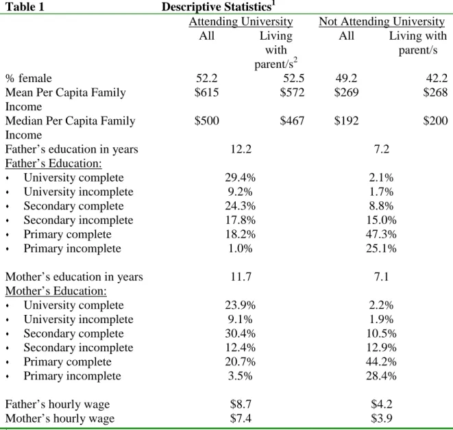
(5) 5. universities have a policy of open enrollment to all high school graduates with no admission exams. In the mid nineties, more than half of the 79 universities in the country were private. However, eighty three percent of the more than one million students were attending public institutions. More than fifty percent of university students were concentrated in Buenos Aires metropolitan area. The largest university is Universidad Nacional de Buenos Aires which is a public institution, and in 1998 had 206,941 undergraduate students. In contrast, the largest private university has less than 17,000 students. Given the high concentration of college students in the Buenos Aires area and the availability of data, we perform the rest of our analysis focusing on this region.. 3. Data and Basic Characteristics of the Population under Study. In this section we attempt to characterize university students and we compare them to their counterparts who are not attending college. We analyze micro data from the May 1998 Permanent Household Survey (EPH). This data covers the city of Buenos Aires and the Greater Buenos Aires region and it is collected by the National Statistical Institute (INDEC). In addition to basic demographic and employment information, the May 1998 survey contains a supplement on education that was administered to all individuals between 5 and 60 years of age. The supplemental survey is organized in three different questionnaires directed to people currently attending school, those who do not attend anymore, and those who never attended. It collects detailed information on the educational history of each person in the household and includes questions that allow us to distinguish between those in public and those in private institutions. Table 1 presents basic statistics for those attending the university and those who are not. We focus on the group of people between 17 and 34 years old without a college degree4. Approximately 18 percent of them are enrolled in the university. The rest has finished or.

(6) 6. abandoned their formal schooling. We observe that women are a majority among university students. The most striking difference between those who attend college and those who do not is per capita household income. The average per capita family income for those who do not attend college is $269 a month. This figure is more than 100 percent higher for university students, reaching $615 per month. Information about their parents is only available if the two generations are still living in the same household. Approximately 80 percent of university students live with at least one parent, but this percentage is only 43 for those who are not in college5. We are aware that this fact might introduce some bias in the results, due perhaps to different household characteristics, so when comparing family background of the two groups we also present information for the whole population as a reference. The distribution of education among parents is very different between groups. Almost half of the university students have fathers who attended college. In contrast, less than 25 percent of men, with ages in the same range as the ages of the fathers of college students, in the total population have some tertiary education. Among those who do not attend college less than 7 percent has a father with education beyond high school. We find a similar pattern among mothers. While 24 percent of women in the total population, with ages in the same range as the ages of the mothers of college students, has some college education, this figure reaches 43 percent among mothers of college students.. TABLE 1 ABOUT HERE. It is clear from Table 1 that a very small proportion of those who have access to college education come from families with low human capital. Less than 20 percent of college students have fathers with primary or lower education. The relationship between parents’ schooling and children’s education is a well-established fact in the literature and it has many dimensions (Schultz, 1988). We can think about parental education as a direct input in the 4. The election of this age range responds to the age distribution of college students in our sample. The results however are not sensitive to changes in the age range we consider. 5 In Argentina is not uncommon for young adults to live with their parents while they are single..

(7) 7. production function of children’s’ education. We can relate it to characteristics of communities and neighborhoods where families locate which can affect the child education too. Clearly, parents’ education can also be seen as related to income, particularly as a proxy for permanent income. Table 2 shows university attendance by income deciles. The majority of university students –almost 70 percent of them- belong to the richest 30 percent of the population. Moreover, only 11 percent of them belong to the bottom half of the income distribution. The results are very similar when we analyze those living with one or both parents. It is possible that this was not always the situation. Using comparable data from 1974 we find that the probability of attending the university was much higher for those at the bottom half of the income distribution. Figure 1 depicts this fact very clearly. While only 11 percent of university students in 1998 belonged to the bottom 50 percent of the income distribution, this figure was almost 30 percent in 1974. This simple descriptive analysis shows an important difference between the socioeconomic background of those enrolled in the university and those who are not. In Argentina, those who attend college come from families located at the top of the income distribution and with high human capital background when compared with those who do not attend college. TABLE 2 ABOUT HERE FIGURE 1 ABOUT HERE. 4. Empirical Results. In this section we further analyze the characteristics of the two groups mentioned in Section 2 by looking at the determinants of university attendance in general, and then by studying the differences between those attending private institutions and those who attend public ones. The strategy we use is as follows. First, we estimate a probit model for university attendance and show which are the principal factors that affect the decision to attend college. Next, we divide those who attend college in two groups: those attending a.

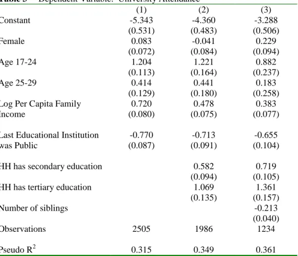
(8) 8. private university and those who attend a public one. We study their family background and analyze if there are differences in the determinants of attending private or public universities.. 4.1 University Attendance. First, we analyze the factors affecting the decision to attend college by estimating a probit model. This is, we model the probability of attending the university by including two sets of explanatory variables. The first set tries to capture personal characteristics such as sex and age. These variables are introduced as dummy variables adopting the value of one when the individual is a woman, is between ages 17 and 24, or ages 25 to 29. A positive sign in the sex variable would imply that women are more likely to attend college. We would expect a higher coefficient for the 17 to 24 age variable than for the 25 to 29 age variable reflecting the fact that those younger are more likely to attend college. The second set of variables tries to describe the family’s socioeconomic background. These variables are: per capita family income, dummy variables for educational level of the head of household (HH), number of siblings living in the parents’ home, and a dummy indicating whether the last educational institution attended was public or private. Given the findings in the previous section we would expect a positive sign associated to the income variable, and a negative one in the number of siblings variable. The greater the education of the head of household, the greater the coefficient we would expect. The variable indicating if the last educational institution was public would discriminate the two groups according to the educational background of the student. Table 3 shows these results. Column (1) includes all current university students, column (2) excludes those individuals that are head of household, and the last column (3) shows the sub-sample of those living with, at least, one parent. In general, sex does not appear to be a significant determinant of university attendance. As suggested in Table 1, we do not find sex gap in educational attainment. Being young seems to increase the.

(9) 9. probability of attending the university when we use any of the samples. After restricting the sample to those living with their parents –a younger group in average- the age coefficient of the dummy variable for people 25 to 29 years old is not statistically significant. Families’ socioeconomic background seems to be an important determinant of college attendance. Our estimates show that the coefficient on per capita family income is positive and significant for all three samples, meaning that individuals coming from families with higher income have a greater probability of attending college, after controlling for other socio-demographic characteristics. Since some individuals in the sample may be working while they are studying, income may be endogenous. In order to check for possible endogeneity of per capita family income we also ran regressions using log of per capita family income but excluding the student’s income. We obtained similar results with both variables suggesting endogeneity is not a problem, so we show the first set of results in Table 3. Further, we performed the Hausman specification test6 and confirmed that log of per capita family income is an exogenous variable. We also included two dummy variables that indicate whether the head of household has a high school degree or a college degree respectively. Both variables enter the equation positively and significantly and the coefficient of the college degree dummy variable is significantly greater than the coefficient on the high school degree variable in agreement with our expectations. As we mentioned before, these variables may be acting as proxies for permanent income and/or may indicate taste or ability towards education. Having attended a private school increases the chances of attending the university too. This finding may reflect differences between public and private institutions that affect the demand for additional education. For those living with their parents we were able to include the effect of having siblings. The probability of attending college is smaller for those with more siblings.. TABLE 3 ABOUT HERE 6. See Hausman (1978)..

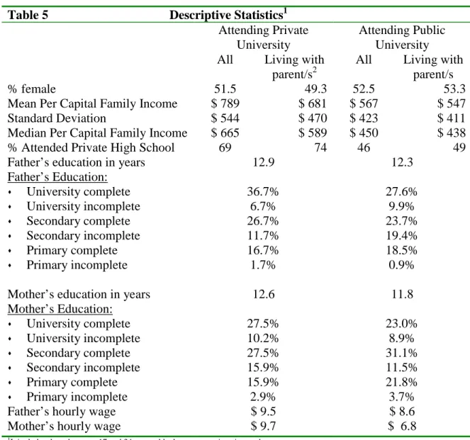
(10) 10. Our results clearly imply that per capita family income is an important determinant of college attendance. To measure its impact on the probability of college attendance, Table 4 shows the change in the predicted probability of university attendance when a change in per capita family income would allocate an average individual in the next decile of the income distribution. For example, when evaluated at the means, a change in per capita family income that moved a person from the seventh to the tenth income decile would more than double the probability of college attendance. It can be seen that the effect of income on the probability of attending the university is larger at the top of the income distribution. For example, doubling per capita income from $50 to $100 will only increase chances of attending the university by around 14 percent. However, increasing per capita income from $250 to $500 will imply an increase of 71 percent, and going from $500 to $1000, will raise the probability 128 percent. Finally, when evaluating at the means, the probability of attending the university is more than one hundred percent higher –other things equal- for those who went to private high schools.. TABLE 4 ABOUT HERE. 4.2 Public and Private Universities Students: Is there any difference?. We have shown that most university students belong to the most affluent sectors of society. In this section we turn to analyze the characteristics of those attending private institutions and those enrolled in public universities. In our sample 22 percent of the students attend private universities. Table 5 shows some basic statistics for both groups. The two groups appear to be similar in many dimensions. The education of students’ parents is not statistically different between the two groups. On average, fathers have approximately 13 years of schooling while mothers have around 12 years. Although, more students in private universities have parents with college degree, it is also true that.

(11) 11. both groups have similar proportions of parents that did not finish high school. Among students in private universities, 69 percent attended private secondary schools. This figure is not low among those in public institutions, almost half of them –46 percent – comes from private high schools, while this figure is only 13 percent among the relevant age group not attending the university. It should be noted that private high schools are not tuition-free and, in some cases, they charge a higher fee than private universities.. TABLE 5 ABOUT HERE. Mean per capita family income of students in public institutions is 72 percent of that of their counterparts in private universities when the whole sample is considered. This figure is slightly larger -80 percent- among students living with their parents. However for both groups, the standard deviation of per capita family income is too large to allow us to draw any strong conclusion about this evidence. Figure 2 shows the whole income distribution using kernel density estimates of log per capita family income for three different groups: those who do not attend college, those in public universities, and those enrolled in private institutions. At first sight it looks as if those who attend the university, in private or public institutions, have higher income than those who do not. Also, while more similar, it seems that income is higher for students in private universities than for students in public ones. To see this more formally, we use the Kolmogorov-Smirnov test to determine differences in the distribution of income for these three groups. We find that per capita family income for those not enrolled in the university is smaller than for those attending college. When comparing students in public and private universities, we also reject the hypothesis that the densities are the same. The test indicates that individuals in private institutions have higher per capita family income than those in public universities. To complete the analysis, Table 6 presents enrollment in public and private universities by per capita family income deciles. As we mentioned before, there are very few students that belong to the bottom 50 percent of the distribution. Less than 12 percent of the students in public universities belongs to the bottom half of the distribution. Surprisingly,.

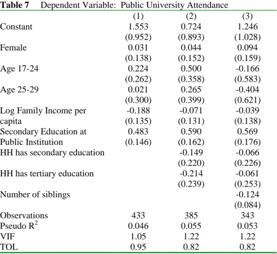
(12) 12. the figure is somewhat higher among students in private institutions, almost 14 percent. Most students, in either public or private universities, belong to the top 30 percent of the income distribution.. FIGURE 2 ABOUT HERE TABLE 6 ABOUT HERE. This preliminary analysis might lead us to conclude that those students coming from wealthier families go to private colleges. However, we did not control for any other characteristics of the population under study. To do so, we estimate a probit model to see how different variables affect the probability of studying in a public institution. Table 7 shows the estimation results. Column (1) includes all available observations; this is including all current university students. As we did in our previous estimates, the next column uses a sub-sample that excludes individuals that are head of household and the last column displays results for the sub-sample of those living at their parents’ home. Following our analysis of university attendance, the explanatory variables are sex, group age dummies, per capita family income, dummy variables for educational level of the head of household, number of siblings living in the household, and a dummy indicating whether the student attended a private or public high school.. TABLE 7 ABOUT HERE. The sex and age dummies do not appear significantly different from zero. The coefficient on per capita family income is negative but is not statistically significant. This finding is very important because it is saying that per capita family income has no effect on the probability of attending a public institution, after controlling for sociodemographic variables. The education of the head of household is not significant either. The coefficient on the number of siblings is negative but not significantly different from zero. Whether the student has attended a public high school has a positive effect on the.

(13) 13. probability of attending a public college. In brief, none of these variables related to personal characteristics, income, and family background appear to distinguish attendance of students to private or public universities. To investigate the possibility that the income variable is collinear with other personal characteristics, Table 7 presents the tolerance (TOL) and variance inflation factors (VIF) for that variable. As a rule of thumb, if the VIF of a variable exceeds 10, that variable is said to be highly collinear. As we can see in Table 7, the VIF of log per capita family income is around one indicating that there is not collinearity between income and personal characteristic variables. Additionally, the TOL equals one if there is no collinearity and approaches zero when there exists near perfect collinearity. Results in Table 7 confirm what we found using the VIF indicator since for all regressions the TOL in near one. The only variable statistically significant in this analysis is the dummy variable indicating attendance to a public high school. As we mentioned in our previous analysis, this finding may reflect differences between public and private institutions, such as quality of education that affects the demand for higher education. Overall, the results of this section are evidence that in Argentina individuals attending college belong to the richest families. Almost 50 percent of the students in public universities belong to the top 20 percent of the income distribution. Moreover, 90 percent of the students in public universities have higher than median per capita family income and almost 50 percent attended private high schools. Since the public university is tuition-free, there is an implicit subsidy to the richest families. We also find that students in public and private universities look similar in many dimensions. This indicates that most of the students in public universities have ability to pay some tuition. Private universities charge fees from around $2,000 to more than $10,000 a year, being the weighted average over $3,300. Tuition fees would cover, at least, part of the public cost of providing higher education. Revenues would free up public funds that can be reallocated toward primary and secondary education, or could be partially used to improve the quality of the public universities.. Furthermore, they could be used to.

(14) 14. develop or extend a system of selective scholarships targeting the most talented students from poor families who otherwise would be unable to attend the university7. As we mentioned, students in public universities seem to have ability to pay while they are completing their studies. However, this may not be the case for all of them all the time. One way to deal with this is to develop a small “need-based” program offering income-contingent loans for those attending higher education public institutions. Students could borrow money to pay tuition or living expenses while they are attending the university and repaid with future incomes. We are aware that student loans present several problems. In particular, they tend to have a low repayment rate due to poor record-keeping, geographic dispersion of borrowers, lack of loan collection incentives, and the difficulty of tracking many students8. However, one of our main empirical findings is that in Argentina the majority of the students in public universities can pay tuition fees. Therefore, a loan program would be small enough to have a close contact between lender and borrower improving record-keeping and easing the tracking of a few students, and in this way, increasing the repayment of loans. A more formal analysis of the design and implementation of this kind of program is beyond the scope of this study; however we could imagine that, even in the case that a good loan program were impossible to be implemented, a system of tuition and scholarships would be better than the current situation. In the next section, we will show that university graduates receive a large wage premium that would allow them to repay borrowed money with future income9.. 5. Returns to Higher Education. 7. In our sample less than 1.4 percent of the students in public universities declared to be receiving a scholarship. 8 For experiences in implementing student loans programs and other reforms in Latin America, see Carlson (1992) and Johnstone et al. (1998) among others. 9 Obviously, these are not the only possible measures one could take in order to solve the inequity of the current educational system in Argentina (See Psacharopuolos et al., 1986, for a description of several policy measures intended to improve equity and efficiency in education)..

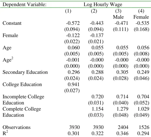
(15) 15. In this section we analyze the returns to university education. University graduates earn substantially higher wages than those who do not have a college degree. Eighty percent of college graduates belong to the top thirty percent of the income distribution. Table 8 shows indices of average earnings by education level for both hourly wages and monthly salaries. Without controlling for any other characteristic, we see that university graduates earn much more than less educated workers. We also estimate an earnings equation using as dependent variable logarithm of hourly wages, in one specification, and logarithm of monthly labor income in a second specification. The explanatory variables are sex, age and its square, and dummy variables reflecting if the individual has high school education or university education. In some of the regressions we split this last variable in those who completed their college education and those who did not. Tables 9 and 10 show the estimates. In all specifications our hypothesis is confirmed. We can see that, on average, university graduates have returns more than three times higher than the returns of those with high school education. The difference is obviously larger when we considered only those that completed their university education. Socio-demographic variables enter the equation as we expected. The earnings-age profile is concave and, other things equal, women earn less than men do.. TABLE 8 ABOUT HERE. University graduates also have a smaller probability of being unemployed. In May 1998, the unemployment rate for university graduates in the Buenos Aires metropolitan area was 5.7 percent while the average unemployment rate excluding them was 15.8 percent. Just as an indication, we want to point out that official figures report that during 1997 the annual cost in public universities was approximately $2,000 per student. This figure is just a little above the average monthly labor income of a college graduate ($ 1,943)..

(16) 16. These findings show that if some students were not able to afford tuition fees while in college, they would be able to postpone their payment until they graduate and begin working.. TABLE 9 ABOUT HERE TABLE 10 ABOUT HERE. 6. Conclusion. In this paper we have analyzed some characteristics of the higher education system in Argentina regarding equity and efficiency. We found that individuals attending the university belong to the top deciles of the income distribution and belong to relatively highly educated families. We did not find that socioeconomic variables are capable of differentiate between those who attend tuition-free public institutions and those attending private colleges. Both groups are very similar with respect to their income and family background. Furthermore, almost half of the students in public universities completed their secondary education in private high schools where they paid tuition. These facts imply that there is an implicit transfer to the richest individuals in society. In Argentina, only a privileged group is able to attend college. Our analysis indicated that poor students are excluded from higher education and they are not able to enjoy the subsidy. The fact that public universities in Argentina are tuition-free does not seem to particularly benefit them. Equity and efficiency of the system can be improved by charging tuition-fees. Complementary to this policy, selective scholarships and student loans could be offered in order to attract the most talented students from poor families. To that end we showed that expected income for college graduates is high and that loan repayment is possible. These policies could eliminate regressive transfers, introduce incentives toward a more efficient educational system, and even increase the number of university graduates..

(17) 17. Acknowledgements - We would like to thank two anonymous referees for helpful suggestions and comments. Alicia Menendez thankfully acknowledges financial support from the John D. and Catherine T. MacArthur Foundation through its Network on Poverty and Inequality in Broader Perspective..

(18) 18. References. Balan, J. & A. Fanelli (1994). Expansión de la oferta universitaria: Nuevas instituciones, nuevos programas. Documento CEDES 106, Serie de Educación Superior, Buenos Aires, Centro de Estudios de Estado y Sociedad. Barro, R. & X. Sala-i-Martin (1995). Economic Growth. New York, McGraw-Hill. Carlson, S. (1992). Private Financing of Higher Education in Latin America and the Caribbean. World Bank, Latin America and the Caribbean Technical Department, Report No. 18 Fernandez, R. & R. Rogerson (1995). On the Political Economy of Education Subsidies. Review of Economic Studies 62, 249-262. Hausman, J. (1978). Specification Tests in Econometrics. Econometrica 46, 1251-1271. Johnstone, B., A. Arora & W. Experton (1998). The Financing and Management of Higher Education: A Status Report on Worldwide Reforms. Mimeo. Psacharopoulos, G., J.P. Tan, & E. Jimenez (1986). Financing Education in Developing Countries: An Exploration of Policy Options. Washington, D.C. World Bank. Rosen, H. S. (1995). Public Finance, Irwin, Auflage, Homewood Ill, 4th edition. Secretaría de Políticas Universitarias (1999). Módulo especial de educación, Encuesta Permanente de Hogares, Mayo 1998. Mimeo. Schultz, T. (1988). Education Investment and Returns. In: Chenery, H. and T.N. Srinivasan, Handbook of Development Economics. Baltimore, MD: Johns Kopkins University Press. Trombetta, A. (1998). Alcances y dimensiones de la educación superior no universitaria en la Argentina, (in spanish). M.A. Thesis..

(19) 19. Table 1. % female Mean Per Capita Family Income Median Per Capita Family Income Father’s education in years Father’s Education: ! University complete ! University incomplete ! Secondary complete ! Secondary incomplete ! Primary complete ! Primary incomplete Mother’s education in years Mother’s Education: ! University complete ! University incomplete ! Secondary complete ! Secondary incomplete ! Primary complete ! Primary incomplete Father’s hourly wage Mother’s hourly wage 1 2. Descriptive Statistics1 Attending University All Living with parent/s2 52.2 52.5 $615 $572 $500. $467. Not Attending University All Living with parent/s 49.2 $269. 42.2 $268. $192. $200. 12.2. 7.2. 29.4% 9.2% 24.3% 17.8% 18.2% 1.0%. 2.1% 1.7% 8.8% 15.0% 47.3% 25.1%. 11.7. 7.1. 23.9% 9.1% 30.4% 12.4% 20.7% 3.5%. 2.2% 1.9% 10.5% 12.9% 44.2% 28.4%. $8.7 $7.4. $4.2 $3.9. It includes those between 17 and 34 years old who are not university graduates. It includes those living with at least one parent or guardian..

(20) 20. Table 2 Distribution of Students Attending University by Income Decile Per Capita Family All Living with at least one Income Decile parent % % 1 1.38 1.75 2 0.69 0.87 3 1.61 1.75 4 3.23 3.50 5 4.15 4.66 6 9.91 10.20 7 10.60 11.66 8 16.82 17.49 9 26.04 25.36 10 25.58 22.74. Figure 1. University Attendance by Income Decile. Attendance Rate. 30 25 20. 1974. 15. 1998. 10 5 0 1. 2. 3. 4. 5. 6. 7. 8. 9. Per Capita Family Income Decile. 10.

(21) 21. Table 3. Dependent Variable: University Attendance (1) (2) Constant -5.343 -4.360 (0.531) (0.483) Female 0.083 -0.041 (0.072) (0.084) Age 17-24 1.204 1.221 (0.113) (0.164) Age 25-29 0.414 0.441 (0.129) (0.180) Log Per Capita Family 0.720 0.478 Income (0.080) (0.075). (3) -3.288 (0.506) 0.229 (0.094) 0.882 (0.237) 0.183 (0.258) 0.383 (0.077). Last Educational Institution was Public. -0.713 (0.091). -0.655 (0.104). 0.582 (0.094) 1.069 (0.135). -0.770 (0.087). HH has secondary education. Observations. 2505. 1986. 0.719 (0.105) 1.361 (0.157) -0.213 (0.040) 1234. Pseudo R2. 0.315. 0.349. 0.361. HH has tertiary education Number of siblings. Note: Figures in parentheses are standard deviations. In all regressions we used as independent variable the log of per capita family income including the income of the university student. To check for the possible endogeneity of this variable we ran the same regressions but using as independent variable the log of per capita family income excluding the income of the university student. We got similar results with both variables, so we show in the tables the first set of regressions. Further, the Hausman test confirmed that the log of per capita family income is exogenous..

(22) 22. Table 4 Change in Predicted Attendance Probability as Income Increases by Decile1 Per Capita Family Income Decile 2 3 4 5 6 7 8 9 10 1. Cumulative 11.75% 8.37% 9.54% 9.07% 11.18% 17.53% 24.07% 41.70% 164.85%. Estimates using the complete sample and evaluated at the means.. 11.75% 20.12% 29.67% 38.74% 49.92% 67.45% 91.52% 133.22% 298.07%.

(23) 23. Descriptive Statistics1 Attending Private University All Living with parent/s2 % female 51.5 49.3 Mean Per Capital Family Income $ 789 $ 681 Standard Deviation $ 544 $ 470 Median Per Capital Family Income $ 665 $ 589 % Attended Private High School 69 74 Father’s education in years 12.9 Father’s Education: 36.7% ! University complete 6.7% ! University incomplete ! Secondary complete 26.7% ! Secondary incomplete 11.7% 16.7% ! Primary complete ! Primary incomplete 1.7% Table 5. Mother’s education in years Mother’s Education: ! University complete ! University incomplete ! Secondary complete ! Secondary incomplete ! Primary complete ! Primary incomplete Father’s hourly wage Mother’s hourly wage 1 2. Attending Public University All Living with parent/s 52.5 53.3 $ 567 $ 547 $ 423 $ 411 $ 450 $ 438 46 49 12.3 27.6% 9.9% 23.7% 19.4% 18.5% 0.9%. 12.6. 11.8. 27.5% 10.2% 27.5% 15.9% 15.9% 2.9% $ 9.5 $ 9.7. 23.0% 8.9% 31.1% 11.5% 21.8% 3.7% $ 8.6 $ 6.8. It includes those between 17 and 34 years old who are not university graduates. It includes those living with at least one parent or guardian..

(24) 24 Not attending University Attending Private University. Attending Public University. .6. .4. .2. 0 0. 5 Log Per Capita Family Income. 10. University Attendance: Kernel Density Estimates. Figure 2. Table 6 Distribution of Students Attending Public and Private Universities by Income Decile Per Capita Family Public Private Income Decile 1 2 3 4 5 6 7 8 9 10. 1.47% 0.88% 1.47% 2.94% 4.41% 11.76% 11.47% 18.53% 26.18% 20.88%. 1.06% 0.00% 2.13% 4.26% 3.19% 3.19% 7.45% 10.64% 25.53% 42.55%.

(25) 25. Table 7. Dependent Variable: Public University Attendance (1) (2) Constant 1.553 0.724 (0.952) (0.893) Female 0.031 0.044 (0.138) (0.152) Age 17-24 0.224 0.500 (0.262) (0.358) Age 25-29 0.021 0.265 (0.300) (0.399) Log Family Income per -0.188 -0.071 capita (0.135) (0.131) Secondary Education at 0.483 0.590 Public Institution (0.146) (0.162) HH has secondary education -0.149 (0.220) HH has tertiary education -0.214 (0.239) Number of siblings Observations Pseudo R2 VIF TOL. 433 0.046 1.05 0.95. 385 0.055 1.22 0.82. (3) 1.246 (1.028) 0.094 (0.159) -0.166 (0.583) -0.404 (0.621) -0.039 (0.138) 0.569 (0.176) -0.066 (0.226) -0.061 (0.253) -0.124 (0.084) 343 0.053 1.22 0.82. Note: Figures in parentheses are standard deviations. In all regressions we used as independent variable the log of per capita family income including the income of the university student. To check for the possible endogeneity of this variable we ran the same regressions but using as independent variable the log of per capita family income excluding the income of the university student. We got similar results with both variables, so we show in the tables the first set of regressions. Further, the Hausman test confirmed that the log of per capita family income is exogenous..

(26) 26. Table 8. Index of Average Labor Earnings by Education Level Average Hourly Wage Average Monthly Wage Primary Incomplete 100 100 Primary Complete 111 138 Secondary Incomplete 122 158 Secondary Complete 164 219 University Incomplete 193 236 University Complete 407 494. Table 9 Dependent Variable: (1) Constant Female Age Age2 Secondary Education College Education. -0.572 (0.094) -0.122 (0.022) 0.060 (0.005) -0.001 (0.000) 0.296 (0.024) 0.941 (0.027). Incomplete College Education Complete College Education Observations R2. 3930 0.301. Log Hourly Wage (2) (3) (4) Male Female -0.443 -0.471 -0.535 (0.094) (0.111) (0.168) -0.137 (0.021) 0.055 0.055 0.056 (0.005) (0.005) (0.008) -0.000 -0.000 -0.000 (0.000) (0.000) (0.000) 0.288 0.305 0.249 (0.024) (0.028) (0.046). 0.720 (0.031) 1.154 (0.033). 0.714 (0.040) 1.279 (0.048). 0.704 (0.052) 1.029 (0.049). 3930 0.322. 2404 0.346. 1526 0.294. Note: Figures in parentheses are standard deviations. We took into account the possible sample bias using Heckman's two step procedure, but the sample bias correction term was not statistically significant. So, we present the results without using that term..

(27) 27. Table 10 Dependent Variable: Log Monthly Wage (1) (2) Constant Female Age Age2 Secondary Education College Education. 4.077 (0.102) -0.483 (0.023) 0.091 (0.005) -0.001 (0.000) 0.388 (0.025) 0.979 (0.029). Incomplete College Education Complete College Education Observations R2. 4119 0.328. (3) (4) Male Female 4.070 3.941 (0.121) (0.178). 4.216 (0.101) -0.499 (0.023) 0.086 (0.005) -0.001 (0.000) 0.380 (0.025). 0.092 (0.006) -0.001 (0.000) 0.384 (0.029). 0.078 (0.009) -0.000 (0.000) 0.364 (0.049). 0.743 (0.033) 1.209 (0.036). 0.675 (0.040) 1.323 (0.050). 0.801 (0.058) 1.101 (0.054). 4119 0.348. 2541 0.358. 1578 0.273. Note: Figures in parentheses are standard deviations. We took into account the possible sample bias using Heckman's two step procedure, but the sample bias correction term was not statistically significant. So, we present the results without using that term..

(28)