Characterization of thermal contacts between heat exchangers and a thermoelectric module by impedance spectroscopy

Texto completo

(1)See discussions, stats, and author profiles for this publication at: https://www.researchgate.net/publication/335711760. Characterization of thermal contacts between heat exchangers and a thermoelectric module by impedance spectroscopy Article in Applied Thermal Engineering · September 2019 DOI: 10.1016/j.applthermaleng.2019.114361. CITATIONS. READS. 0. 26. 3 authors, including: Braulio Beltrán-Pitarch. Jorge García-Cañadas. Universitat Jaume I. Universitat Jaume I. 9 PUBLICATIONS 18 CITATIONS. 61 PUBLICATIONS 833 CITATIONS. SEE PROFILE. All content following this page was uploaded by Braulio Beltrán-Pitarch on 14 September 2019.. The user has requested enhancement of the downloaded file.. SEE PROFILE.

(2) This document is the unedited Author’s version of a Submitted Work that was subsequently accepted for publication in Applied Thermal Engineering. To access the final edited and published work see https://doi.org/10.1016/j.applthermaleng.2019.114361. Characterization of thermal contacts between heat exchangers and a thermoelectric module by impedance spectroscopy Braulio Beltrán-Pitarch1 and Jorge García-Cañadas1,* 1Department. *e-mail:. of Industrial Systems Engineering and Design, Universitat Jaume I, Campus del Riu Sec, 12071 Castellón, Spain. [email protected]. Heat to electricity energy conversion efficiency of a thermoelectric (TE) device is not only influenced by the TE materials properties, but it also depends on the temperature difference between both sides of the TE legs. Keeping this temperature difference as close as possible to the temperature difference between the heat sink and the heat source is crucial to maximize the TE device performance. However, achieving this is quite difficult, mainly due to the thermal contact resistance at the interfaces between the TE module and the heat sink/source. In this study, it is analyzed the effect of this thermal contact resistance on the impedance spectroscopy response of a TE module that is thermally contacted by two copper blocks, which act as heat exchangers. A new theoretical model (equivalent circuit) that takes into account the thermal contact resistance is developed, which includes two new elements that depend on this parameter. The equivalent circuit is validated with experimental impedance measurements where the thermal contact is varied. It is demonstrated that using this equivalent circuit the thermal contact resistance can be easily determined, which opens up the possibility of using impedance spectroscopy as a tool to quantify and monitor this crucial property for the TE device performance. Keywords: Thermal contact resistance, thermal interface, impedance spectroscopy, heat sink, heat exchangers.. I. INTRODUCTION A thermoelectric (TE) device that operates converting heat into electricity is typically contacted to a heat source and a heat sink under operating conditions. The heat to electricity energy conversion efficiency of the device depends on the TE properties of its TE materials, and also on the temperature difference at their edges. In the latter case, in order to maximize the efficiency it is important to keep the temperature at the edges of the TE materials as close as possible to the temperature of the heat sink and the heat source contacted at each of the sides of the device..

(3) Due to the thermal contact resistance existing at the interface between two solids [1], the temperature at the surface of the heat exchangers differs from that at the surface of the alumina ceramics (or similar electrically insulating material) which are usually the most external layers of a TE device. In order to minimize the thermal contact resistance different parameters can significantly influence, such as the contact pressure and the roughness of the surfaces that enter into contact [2,3]. In addition, it is typically adopted the use of different thermal interface materials (e.g. thermal grease, graphite sheets), which can significantly decrease the thermal contact resistance and thus increase the system efficiency [2–4].. The thermal contact resistance between two materials is typically determined by measuring the temperature drop at the interface of the materials when heat flows through the interface. This is performed using several thermocouples and materials with known thermal conductivity [5–8]. In many cases, it is also common the use of an infrared camera instead of thermocouples to determine the temperature profile across the junction [9,10]. Alternatively, thermal contact resistances can be also determined by fitting the temperature profile recorded in one solid when another solid in contact is heated by a laser beam [11,12].. We present her a new method to determine the thermal contact resistance between the external surfaces of a TE device and the heat exchangers. The method is based on the use of impedance spectroscopy. This method has recently received significant attention in the field of TEs due to its capability to characterize TE materials and modules [13–18]. Especially interesting are different studies that have shown the high sensitivity of the impedance method to any thermal phenomena taking place at the surroundings of the TE module, such as convection [15,19], radiation [15], or conduction through other material in contact with the module [20,21]. Due to this, it is expected that a thermal contact resistance will also produce a significant influence in the impedance response, and in fact this was observed in a recent study [22]. However, this recent article did not develop any equivalent circuit to account for the thermal contact resistance influence. On the other hand, a previous study [21] considered the presence of a thermal contact in the impedance response in the context of a thermal quadrupole analysis, but a detailed analysis of the thermal contact resistance and a procedure for its determination was missing.. 2.

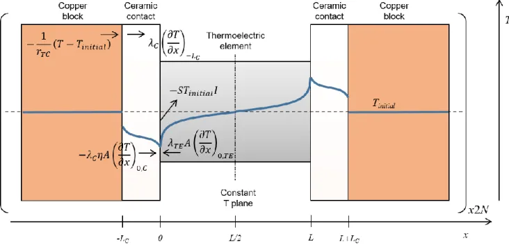
(4) In this work, a new impedance theoretical model (equivalent circuit), which includes the presence of thermal contact resistances between heat exchangers and the outer ceramic surfaces of a TE module has been developed and experimentally validated. The new equivalent circuit is obtained by solving the heat equation in the frequency domain. Using this equivalent circuit, the thermal contact resistances between the heat exchangers and the TE module can be determined from an impedance spectroscopy measurement of the module under suspended conditions and another measurement of the module contacted with the heat exchangers, given that the average Seebeck coefficient of the device thermoelements is known.. II. THEORETICAL MODEL The theoretical model adopted for the interpretation of the impedance response with the presence of thermal contact resistances is shown in Fig. 1. This one-dimensional model consists of 2N TE legs of certain length L and area A, being N the number of TE couples. Each leg is sandwiched between two ceramic pieces of length LC and an area per TE leg A/η, being η the filling factor of the TE module, which is the ratio between the area of the ceramic plate occupied by the TE legs [(2N+)A, being  the number of legs removed to attach the leads of the device, typically 2] and the actual area of the ceramics. The thermal influence of the metallic strips (usually copper electrodes) that interconnect the TE legs is neglected due to their high thermal conductivity and small thickness. The model does not consider spreading-constriction effects [15,23] of the heat flow due to the difference of area between TE legs and ceramics for simplicity, but it considers the difference between the areas (introduced by the filling factor η). All the TE properties are considered independent on temperature and Joule effect is neglected due to the high electrical conductivity of TE materials and the small current amplitude used during the impedance spectroscopy measurements. The system is also considered adiabatic (no radiation and convection losses). At the outer ceramic surfaces a thermal contact resistance and a perfect heat sink condition are considered (see Fig. 1).. 3.

(5) Fig. 1. Thermal model employed in the theoretical analysis. The arrows indicate the direction of the conducting heat fluxes appearing at the different junctions, considering a positive value of both the electrical current and the Seebeck coefficient. For the Peltier heat, the arrows point out of the junction when heat is absorbed. The solid line depicts qualitatively a possible thermal profile. The dotted line shows the plane where the temperature remains constant at any time due to the symmetry of the system. The dashed line indicates the initial temperature.. The impedance function Z=V/I of a TE module as defined above and considering the symmetry of the system is given by,. 𝑍=. 𝑉(0) − 𝑉(𝐿) 𝑆[𝑇(𝐿) − 𝑇(0)] 2𝑆[𝑇(0) − 𝑇𝑖𝑛𝑖𝑡𝑖𝑎𝑙 ] = 𝑅𝛺 + 2𝑁 = 𝑅𝛺 − 2𝑁 , 𝐼0 𝐼0 𝐼0. (1). where V(0) and V(L) are the voltages at x=0 and x=L, respectively, I0 is the electrical current flowing through the device at x=0, RΩ is the total ohmic resistance, which includes the contribution of all the TE legs of the TE module, the metallic strips, the leads, and the electrical contact resistances, S is the average absolute Seebeck coefficient of all the TE legs, and T(0), T(L), and Tinitial are the temperatures at x=0, x=L, and the initial temperature, respectively. It should be noted from Eq. (1) that due to the symmetry of the system with respect to the constant temperature plane (x=L/2), the temperature difference across the TE leg can be determined from the value of the temperature at x=0.. To determine the variation with frequency of T(0), the heat equation of the system must be solved in the frequency domain,. 4.

(6) 𝜕 2 𝜃 𝑗𝜔 − 𝜃 = 0, 𝜕𝑥 2 𝛼𝑖. (2). where θ=L[T-Tinitial]) is the Laplace transform of the temperature with respect to the initial temperature, j=(-1)0.5 is the imaginary number, ω is the angular frequency (defined as ω=2πf, where f is the frequency) and αi is the average thermal diffusivity of the TE legs (i=TE) or the ceramic plates (i=C).. The solution of Eq. (2) and its derivative are given by, 𝑥 𝑗𝜔 0.5 𝑥 𝑗𝜔 0.5 𝜃 = 𝐶1,𝑖 𝑠𝑖𝑛ℎ [ ( ) ] + 𝐶2,𝑖 𝑐𝑜𝑠ℎ [ ( ) ] 𝐿𝑖 𝜔𝑖 𝐿𝑖 𝜔𝑖. (3). 𝜕𝜃 1 𝑗𝜔 0.5 𝑥 𝑗𝜔 0.5 𝑥 𝑗𝜔 0.5 = ( ) {𝐶1,𝑖 𝑐𝑜𝑠ℎ [ ( ) ] + 𝐶2,𝑖 𝑠𝑖𝑛ℎ [ ( ) ]} 𝜕𝑥 𝐿𝑖 𝜔𝑖 𝐿𝑖 𝜔𝑖 𝐿𝑖 𝜔𝑖. (4). where Li is the half length of the TE legs (i=TE) or the thickness of the ceramic plate (i=C), ωi is the characteristic angular frequency of each material (being ωi=αi/Li2), and C1,i and C2,i are constants.. The following boundary conditions are applied (see Fig. 1),. 𝜕𝜃. −𝜃(−𝐿𝐶 )𝐶 + 𝑟𝑇𝐶 𝜆𝐶 ( ). 𝜕𝑥 −𝐿𝐶. = 0, at x=-LC. (5). 𝜃(0) 𝑇𝐸 = 𝜃(0)𝐶 , temperature continuity at x=0 𝜕𝜃. −𝑆𝑇𝑖𝑛𝑖𝑡𝑖𝑎𝑙 𝑖0 − 𝜆𝐶 𝜂𝐴 ( ). 𝜕𝑥 0,𝐶. 𝜕𝜃. + 𝜆 𝑇𝐸 𝐴 ( ). 𝜃(𝐿/2) = 0, at x=L/2. 𝜕𝑥 0,𝑇𝐸. = 0, at x=0. (6) (7) (8). where i0 is the Laplace transform of the current (i0=L[I0]) at x=0, and λC and λTE the thermal conductivity of the ceramic plates and the TE legs, respectively. In addition, rTC is the thermal contact resistance between the TE module and the heat exchangers.. Using the boundary conditions given by Eqs. (5) to (8) in Eqs. (3) and (4), the Laplace transform of the temperature at x=0 takes the form,. 5.

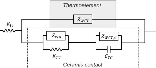
(7) 𝜃(0) =. −𝑆𝑇𝑖𝑛𝑖𝑡𝑖𝑎𝑙 𝑖0 𝜆 𝑇𝐸 𝑗𝜔 0.5 𝑗𝜔 0.5 ( ) coth ( ) 𝐴 𝐿 𝑇𝐸 𝜔 𝑇𝐸 𝜔 𝑇𝐸 { −1. 𝑗𝜔 0.5 𝑟𝑇𝐶 𝜆𝐶 𝑗𝜔 0.5 𝑗𝜔 0.5 0.5 cosh ( ) ( ) ( ) + sinh 𝜆𝐶 𝑗𝜔 𝜔𝐶 𝐿𝐶 𝜔𝐶 𝜔𝐶 + ( ) . 𝐿𝐶 𝜔𝐶 𝑗𝜔 0.5 𝑗𝜔 0.5 𝑟𝑇𝐶 𝜆𝐶 𝑗𝜔 0.5 ( ) cosh ( ) + sinh ( ) 𝐿𝐶 𝜔𝐶 𝜔𝐶 𝜔𝐶 }. (9). Using Eq. (1) and reorganizing the different terms, we reach the impedance expression,. −1. 𝑍 = 𝑅𝛺 + {𝑍𝑊𝐶𝑇 −1 + [(𝑍𝑊𝑎 −1 + 𝑅𝑇𝐶 −1 ). −1 −1 −1. + (𝑍𝑊𝐶𝑇,𝐶 −1 + 𝑍𝐶𝑇𝐶 −1 ) ] }. (10). where the elements in Eq. (10) are,. 𝑍𝑊𝐶𝑇. 𝑍𝑊𝑎. 2𝑁𝑆 2 𝑇𝑖𝑛𝑖𝑡𝑖𝑎𝑙 𝐿 𝑗𝜔 −0.5 𝑗𝜔 0.5 ( ) ) ], = 𝑡𝑎𝑛ℎ [( 𝜆 𝑇𝐸 𝐴 𝜔 𝑇𝐸 𝜔 𝑇𝐸. 4𝑁𝑆 2 𝑇𝑖𝑛𝑖𝑡𝑖𝑎𝑙 𝐿𝐶 𝜂 𝑗𝜔 −0.5 𝑗𝜔 0.5 ( ) [( ) ], = 𝑐𝑜𝑡ℎ 𝜆𝐶 𝐴 𝜔𝐶 𝜔𝐶. 𝑅𝑇𝐶 =. 4𝑁𝑆 2 𝑇𝑖𝑛𝑖𝑡𝑖𝑎𝑙 𝑟𝑇𝐶 𝜂 , 𝐴. (12). (13). 4𝑁𝑆 2 𝑇𝑖𝑛𝑖𝑡𝑖𝑎𝑙 𝐿𝐶 𝜂 𝑗𝜔 −0.5 𝑗𝜔 0.5 ( ) 𝑡𝑎𝑛ℎ [( ) ] , 𝜆𝐶 𝐴 𝜔𝐶 𝜔𝐶. (14). 4𝑁𝑆 2 𝑇𝑖𝑛𝑖𝑡𝑖𝑎𝑙 𝐿𝐶 2 𝜂 𝑗𝜔 −1 4𝑁𝑆 2 𝑇𝑖𝑛𝑖𝑡𝑖𝑎𝑙 𝜂 1 ( ) = , 𝜔𝐶 𝜆𝐶 𝜌𝐶 𝐶𝑝,𝐶 𝐴𝑟𝑇𝐶 𝑗𝜔 𝜆𝐶 2 𝐴𝑟𝑇𝐶. (15). 𝑍𝑊𝐶𝑇,𝐶 =. 𝑍𝐶𝑇𝐶 =. (11). being ρC and Cp,C the mass density and specific heat of the ceramic material, respectively. Eq. (10) can be represented by the equivalent circuit shown in Fig. 2.. The new equivalent circuit of Fig. 2 has similarities to that obtained in our previous work where the TE module was simply suspended (without the presence of heat exchangers) and the effect of convection was considered at the outer ceramic surfaces [19]. Unlike the previous work, due to the presence of the heat exchangers here a thermal contact resistance boundary condition and no temperature variation in the heat exchangers is considered (see Fig.. 6.

(8) 1). This produces the existence of a thermal contact resistance instead of the convection heat transfer coefficient in the resistance and capacitance elements (RTC and CTC, which in the case of convection were Rconv and Cconv). In addition, the filling factor η, which in the previous article was added to account for convection effects produced at the external area of the ceramic plates that was larger than the total legs area, and only affected the Rconv and Cconv impedance elements, now it also affects the Warburg elements related to the ceramic plates (ZWa and ZWCT,C). This is due to the consideration of the difference in areas between all the legs and the ceramic plates [Fig. 1 and Eq. (7)], as also occurred when this was considered in another of our previous studies [15]. The inclusion of η in the elements related to the ceramic plates must be used as a general rule, since in this way the thermal effects in the total area of the ceramic plates is considered, not only in the part covered by the TE legs.. Fig. 2. Equivalent circuit corresponding to a thermoelectric device contacted by two heat sinks, existing a thermal contact resistance at the contact. The equivalent circuit elements framed by the dotted line are related to the external ceramic plates. The elements framed by the solid line relate to the thermoelements.. It can be observed that for the case of an ideal thermal contact (rTC→0), the impedance from the equivalent circuit element RTC→0 and CTC→∞, thus, the equivalent circuit in Fig. 2 reduces to the parallel combination of ZWCT,C with ZWCT, connected in series with RΩ, whose response can be observed in the simulations on Fig. 3 (more clearly in the magnification of Fig. 3c). In this case, the constant temperature Warburg element from the ceramics ZWCT,C represents the diffusion of heat within the ceramic from the Cu/TE junctions, which is completely removed by the effect of the heat sinks (heat exchangers) when they are reached, producing no temperature change at the outer ceramic surfaces (constant-temperature boundary). In the opposite case, if rTC→∞, then RTC→∞ and CTC→0,. 7.

(9) and the equivalent circuit of Fig. 2 will reduce to the parallel combination of ZWa with ZWCT, connected in series with RΩ, which is the response obtained for a suspended module under adiabatic conditions [13], as shown in the simulations of Fig. 3. In this case, the huge thermal contact resistance blocks the heat transfer towards the heat exchangers and all the heat is accumulated in the ceramic layers. Apart from these two extreme cases, it can be observed from the simulations of Fig. 3, where the thermal contact resistance value has been systematically reduced, that the presence of the thermal contact resistance introduces significant differences in the semicircle part of the impedance response, which considerably reduces when rTC decreases. However, at high frequencies (bottom left part), the 45 degrees straight line feature is the same in all cases, which relates with the diffusion of heat from the TE legs ends towards the ceramic layers, until the end of the ceramic is reached. Once the effect of this boundary is sensed, around the turnover angular frequency ω=2πωC (see Fig. 3c), the effect of the thermal contact resistance starts to be observed when the frequencies are decreased (moving to the right side).. Fig. 3. (a) Impedance spectroscopy simulations from 10 mHz to 10 kHz for four different thermal contact resistance values for the contacts between a thermoelectric module and two heat sinks. The plots in (b) and (c) are magnifications of the bottom left part (same axis units). Typical values for commercial Bi2Te3 thermoelectric modules were used (N=127, S=180 µVK-1, ρTE=1 mΩcm, λTE=1.5 Wm-1K-1, αTE=0.37 mm2s-1, L=1.2 mm, λC=20 Wm-1K-1, αC=10 mm2s-1, LC=0.7 mm, A=1.69 mm2, T=300 K, η=0.268).. 8.

(10) In the new equivalent circuit (Fig. 2), two new elements appear for the first time, RTC and CTC. RTC=4NS2TinitialrTCη/A is the thermal contact electrical resistance, in which the only thermal parameter that influences its value is rTC. Its physical meaning is related to the electrical losses in the system due to the blockage of the heat flow by the thermal contacts, which causes a higher temperature modification of the temperature difference at the edges of the thermoelements, since heat removal by the heat exchangers is less efficient. High rTC values will considerably block the heat flow and high RTC values will result, as shown in Fig. 3a. In contrast, low rTC values will allow the heat to flow and very small RTC values will result. It should be noted that RTC has a huge influence on the dc resistance Rdc, which accounts for the total losses of the system. Note that Rdc is the value adopted by the impedance response [Eq. (10)] when ω→0 (steady state), and corresponds to Rdc=RΩ+[RTE-1+(RTC+RC)-1]-1, being RTE=2NS2TinitialL/(λTEA) the TE resistance, coming from the ZWCT element, and RC=4NS2TinitialLCη/(λCA) the TE resistance induced by the ceramic layers, coming from the ZWCT,C element [13,24]. Rdc can be easily identified from the impedance plots, since it is the low frequency intercept with the real axis. It is remarkable that Rdc is also influenced here by RC, which was not the case in the impedance response of modules under suspended conditions [13,15,19]. The other new element is a thermal contact capacitance CTC=λCρCCp,CArTC/(4NS2Tinitialη) since adopts the form of a capacitor [ZCTC=(jωCTC)-1]. It is influenced by two thermal parameters, rTC and the thermal effusivity e=(λCρCCp,C)0.5. The latter is a parameter that define the ability of materials to exchange heat with the surroundings [25]. Both rTC and e determine the temperature of the junction at the side of the ceramic layer, which is eventually governed by the heat release/accumulation at the interface. When rTC increases, CTC also increases and the impedance response shows a growth in their absolute imaginary part values at ω<<2πωC (see Fig. 3), which is related to a higher temperature drop at the interface, produced by a more prominent heat release/accumulation. Although the effect of the variation of e is not shown in Fig. 3, it will also provide a higher CTC value if increased, producing the same result as the rTC increase.. Using RTE, RC, and RTC, the equivalent circuit elements of Eqs. (11), (12), (14) and (15), can be rewritten as,. 9.

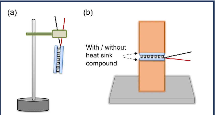
(11) 𝑗𝜔 −0.5 𝑗𝜔 0.5 ) ) ], 𝑍𝑊𝐶𝑇 = 𝑅𝑇𝐸 ( 𝑡𝑎𝑛ℎ [( 𝜔 𝑇𝐸 𝜔 𝑇𝐸 𝑍𝑊𝑎 = 𝑅𝐶 (. 𝑗𝜔 −0.5 𝑗𝜔 0.5 ) 𝑐𝑜𝑡ℎ [( ) ] , 𝜔𝐶 𝜔𝐶. 𝑗𝜔 −0.5 𝑗𝜔 0.5 𝑍𝑊𝐶𝑇,𝐶 = 𝑅𝐶 ( ) 𝑡𝑎𝑛ℎ [( ) ] , 𝜔𝐶 𝜔𝐶 𝑍𝐶𝑇𝐶. 𝑅𝐶 2 𝑗𝜔 −1 ( ) . = 𝑅𝑇𝐶 𝜔𝐶. (16). (17). (18). (19). In this way, CTC can be obtained once RC and RTC are known, which then simplifies the fitting, since CTC is no longer a variable. Hence, these equations will be used to perform fittings to experimental results. This simplification cannot be easily implemented in the standard impedance fittings programs (e.g. Zview), and hence, MATLAB will be employed for this purpose.. III. EXPERIMENTAL VALIDATION In order to experimentally validate the model developed in the previous section, we performed impedance measurements using a 40 mm x 40 mm Bi2Te3 commercial TE module from European Thermodynamics (Ref. 6937080), which is formed by 127 couples of 1.3 mm x 1.3 mm x 1.2 mm legs and 0.7 mm ceramic thickness. A first impedance spectroscopy measurement was performed to this module suspended in vacuum conditions at a pressure of 1.0x10-3 mbar to eliminate convection losses [see Fig. 4(a)]. Then, the TE module was measured in air (without vacuum) sandwiched between two copper blocks, which acted as heat exchangers [see Fig. 4(b)]. The copper blocks are 40 mm x 40 mm x 50 mm size and have a mass of 712 g, which implies a pressure in the system of 4.36 kPa. The TE module sandwiched by the Cu blocks was measured without (only mechanical contact) and with heat sink compound (thermal grease) from RS (Ref. 217-3835) added at the contacts. In order to have a good initial thermal contact, the copper blocks were slightly polished with 800 grit size silicon carbide sandpaper before being assembled. All the impedance measurements were performed using a PGSTAT30 potentiostat (Metrohm Autolab B. V.) equipped with a FRA2 impedance module and a BOOSTER10A at 0 A dc current and 50 mA ac current amplitude, measuring 50 logarithmically distributed frequency steps between 20 mHz and 20 kHz. The typical inductive response that appears at high frequencies was neglected in the measurements, and only the frequency. 10.

(12) range from 20 mHz to 40.47 Hz was analyzed, unless otherwise stated. Fittings to the experimental results were performed using the equivalent circuit of Fig. 2 [Eqs. (16)-(19)] with Matlab software. The code employed is available in the supplementary information All the measurements were performed inside a metallic vacuum chamber that acted as Faraday cage and at room temperature.. Fig. 4. Schematic of the experimental setups for the measurements performed to (a) a module suspended, and (b) the same module in contact with two copper blocks acting as heat exchangers and contacted with and without heat sink compound.. Fig. 5 shows the experimental impedance spectroscopy measurements (dots) and their associated fittings (lines). It can be clearly observed that the same trend observed in the simulations from Fig. 3 occurs now in Fig. 5 as the thermal contact resistance is modified. In addition, all the fittings performed are in good agreement with the experimental results. It should be noted that the fitting to the suspended module experiment was carried out discarding the effect of the thermal contact resistance, i.e. with an equivalent circuit formed by the ohmic resistance (RΩ) in series with the parallel combination of ZWCT and ZWa [13]. From this fitting, RTE and RC, were obtained (see Table 1) and used in the fittings of the other experiments that include a thermal contact resistance. This was performed since otherwise it is not possible to fit the complete equivalent circuit (Fig. 2) due to the large number of variables. Note that both RTE and RC only depend on materials properties, which do not change along the different setups.. 11.

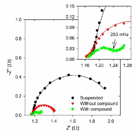
(13) Fig. 5. Experimental impedance spectra (dots) of a commercial Bi2Te3 thermoelectric module suspended in vacuum and in contact in air with two copper blocks (with and without heat sink compound). The lines represent the fittings performed with the equivalent circuit of Fig. 2. The inset shows the magnification at medium and high frequencies.. The fitting results to the experiments in Fig. 5 can be seen in Table 1. From the fitted value of RTC the thermal contact resistance rTC can be determined if the average absolute Seebeck coefficient of the thermoelements is known [see Eq. (13)]. Hence, in order to determine rTC, the Seebeck coefficient of the TE module was measured from an open-circuit voltage vs. temperature difference curve, obtaining a value of 186.42 μVK-1. The obtained thermal contact resistance values are 3.2x10-4 and 1.7x10-5 m2KW-1 (see Table 1) for the thermal contacts without and with heat sink compound, respectively, which are in good agreement with literature values [4,8,26].. Table 1. Fitting parameters obtained from the fittings to the experimental measurements of Fig. 5 of a commercial Bi2Te3 thermoelectric module suspended under vacuum and in contact with two copper blocks at room conditions (T=298.0 K), with and without using heat sink compound. The errors provided from the fittings are given between brackets. The thermal contact resistances were calculated using Eq. (13) and the Seebeck coefficient value of 186.42 μVK-1 was experimentally obtained.. Suspended w/o compound w/ compound. RΩ (Ω). RTE (Ω). 1.16 (0.16%) 1.16 (0.04%) 1.16 (0.04%). 0.869 (0.72%) -----. ωTE (rads-1) 0.392 (14.53%) 0.245 (5.06%) 0.306 (33.23%). RC (Ω) 0.0812 (18.03%) -----. ωC (rads-1) 5.48 (20.49%) 5.99 (3.64%) 5.38 (16.01%). CTC (F). RTC (Ω). rTC (m2KW-1). ---. ---. ---. 0.267 (0.9%) 0.0142 (37.2%). 3.2x10-4. 6.76 0.40. 1.7x10-5. 12.

(14) It can be observed from the spectrum of the module contacted to the copper blocks using thermal grease (inset of Fig. 5) that the impedance response deviates from that predicted by the equivalent circuit at low frequencies, showing an increase of the absolute value of the imaginary part instead of tending to zero. This occurs since the copper blocks are not large enough to keep their temperature constant, and since the thermal contact has improved the heat can transfer more easily to the copper blocks producing their temperature variation. For this reason, the fitting in this case was performed from 253 mHz to 40.47 Hz (see inset of Fig. 5). Note that this was not observed in the module without heat sink compound due to its larger thermal contact resistance. Moreover, it can be also found from Table 1 that the fitting errors are higher with heat sink compound than in the case without it, which is attributed to the deviation from the equivalent circuit produced by the temperature change in the copper blocks.. IV. CONCLUSIONS In order to study the effect of a thermal contact resistance in the impedance signal of a TE module, a new theoretical model (equivalent circuit) has been developed considering a TE device sandwiched between two copper blocks, which act as heat exchangers. Two new elements in the equivalent circuit influenced by the thermal contact resistance appear in the analysis: a thermal contact electrical resistance and a thermal contact capacitance. The theoretical model is validated by experimental measurements performed to a commercial Bi2Te3 module contacted by copper blocks. It was found that the impedance response significantly differs from that of the module suspended (not in contact with the heat exchangers) under adiabatic conditions. The experimental results are in good agreement with the behavior predicted by the new theoretical model. Moreover, it is possible to quantify the value of the thermal contact resistance. This can be performed from a measurement of the module in vacuum and the knowledge of the average Seebeck coefficient of its thermoelements before being measured in contact with the heat exchangers. A thermal contact resistance value of 1.7x10-5 m2KW-1 was obtained when the module was contacted with heat sink compound, which is in agreement with literature values. This opens up the possibility of using impedance spectroscopy as a tool to quantify and monitor the thermal contact resistance, which is a key parameter in the performance of TE devices.. ACKNOWLEDGMENTS. 13.

(15) The authors acknowledge financial support from the Spanish Agencia Estatal de Investigación under the Ramón y Cajal program (RYC-2013-13970), from the Generalitat Valencian and the European Social Fund under the ACIF program (ACIF/2018/233) from the Universitat Jaume I under the project UJI-A2016-08, and the technical support of Raquel Oliver Valls and José Ortega Herreros. European Thermodynamics is also acknowledged for providing the thermoelectric devices.. REFERENCES [1]. Incropera FP, DeWitt DP. Fundamentals of Heat and Mass Transfer. USA: John Wiley & Sons; 2002.. [2]. Karthick K, Suresh S, Singh H, Joy GC, Dhanuskodi R. Theoretical and experimental evaluation of thermal interface materials and other influencing parameters for thermoelectric generator system. Renew Energy 2019;134:25–43. doi:10.1016/j.renene.2018.10.109.. [3]. Wang S, Xie T, Xie H. Experimental study of the effects of the thermal contact resistance on the performance of thermoelectric generator. Appl Therm Eng 2018;130:847–53. doi:10.1016/J.APPLTHERMALENG.2017.11.036.. [4]. Karthick K, Joy GC, Suresh S, Dhanuskodi R. Impact of Thermal Interface Materials for Thermoelectric Generator Systems. J Electron Mater 2018;47:5763–72. doi:10.1007/s11664-018-6496-y.. [5]. Rosochowska M, Balendra R, Chodnikiewicz K. Measurements of thermal contact conductance. J Mater Process Technol 2003;135:204–10. doi:10.1016/S0924-0136(02)00897-X.. [6]. Azuma K, Hatakeyama T, Nakagawa S. Measurement of surface roughness dependence of thermal contact resistance under low pressure condition. 2015 Int. Conf. Electron. Packag. iMAPS All Asia Conf., IEEE; 2015, p. 381–4. doi:10.1109/ICEP-IAAC.2015.7111040.. [7]. Misra P, Nagaraju J. Test facility for simultaneous measurement of electrical and thermal contact resistance. Rev Sci Instrum 2004;75:2625–30. doi:10.1063/1.1775316.. [8]. Xian Y, Zhang P, Zhai S, Yuan P, Yang D. Experimental characterization methods for thermal contact resistance: A review. Appl Therm Eng 2018;130:1530–48. doi:10.1016/j.applthermaleng.2017.10.163.. [9]. Fieberg C, Kneer R. Determination of thermal contact resistance from transient temperature measurements. Int J Heat Mass Transf 2008;51:1017–23. doi:10.1016/J.IJHEATMASSTRANSFER.2007.05.004.. [10]. Warzoha RJ, Donovan BF. High resolution steady-state measurements of thermal contact resistance across thermal interface material junctions. Rev Sci Instrum 2017;88:094901. doi:10.1063/1.5001835.. [11]. Ohsone Y, Wu G, Dryden J, Zok F, Majumdar A. Optical Measurement of Thermal Contact Conductance Between Wafer-Like Thin Solid Samples. J Heat Transfer 1999;121:954. doi:10.1115/1.2826086.. [12]. Dongmei B, Huanxin C, Shanjian L, Limei S. Measurement of thermal diffusivity/thermal contact resistance using laser photothermal method at cryogenic temperatures. Appl Therm Eng 2017;111:768–75. doi:10.1016/J.APPLTHERMALENG.2016.07.188.. [13]. García-Cañadas J, Min G. Impedance spectroscopy models for the complete characterization of thermoelectric materials. J Appl Phys 2014;116:174510. doi:10.1063/1.4901213.. [14]. Beltrán-Pitarch B, Prado-Gonjal J, Powell A V., Ziolkowski P, García-Cañadas J. Thermal conductivity, electrical resistivity, and dimensionless figure of merit (ZT) determination of thermoelectric materials by impedance spectroscopy up to 250 °C. J Appl Phys 2018;124:025105. doi:10.1063/1.5036937.. [15]. Mesalam R, Williams HR, Ambrosi RM, García-Cañadas J, Stephenson K. Towards a comprehensive model for characterising and assessing thermoelectric modules by impedance spectroscopy. Appl Energy 2018;226:1208–18. doi:10.1016/j.apenergy.2018.05.041.. [16]. Yoo C-Y, Kim Y, Hwang J, Yoon H, Cho BJ, Min G, et al. Impedance spectroscopy for assessment of. 14.

(16) thermoelectric module properties under a practical operating temperature. Energy 2017;152:834–9. doi:10.1016/j.energy.2017.12.014. [17]. Apertet Y, Ouerdane H. Small-signal model for frequency analysis of thermoelectric systems. Energy Convers Manag 2017;149:564–9. doi:10.1016/j.enconman.2017.07.061.. [18]. Hasegawa Y, Otsuka M. Temperature dependence of dimensionless figure of merit of a thermoelectric module estimated by impedance spectroscopy. AIP Adv 2018;8:075222. doi:10.1063/1.5040181.. [19]. Beltrán-Pitarch B, García-Cañadas J. Influence of convection at outer ceramic surfaces on the characterization of thermoelectric modules by impedance spectroscopy. J Appl Phys 2018;123:084505. doi:10.1063/1.5019881.. [20]. Beltrán-Pitarch B, Márquez-García L, Min G, García-Cañadas J. Measurement of thermal conductivity and thermal diffusivity using a thermoelectric module. Meas Sci Technol 2017;28:045902.. [21]. De Marchi A, Giaretto V. The Peltier driven frequency domain approach in thermal analysis. Rev Sci Instrum 2014;85:103904. doi:10.1063/1.4897189.. [22]. Boldrini S, Ferrario A, Miozzo A. Investigation of Pulsed Thermoelectric Performance by Impedance Spectroscopy. J Electron Mater 2019. doi:10.1007/s11664-018-06922-9.. [23]. Casalegno F, De Marchi A, Giaretto V. Frequency domain analysis of spreading-constriction thermal impedance. Rev Sci Instrum 2013;84:024901. doi:doi:http://dx.doi.org/10.1063/1.4789765.. [24]. García-Cañadas J, Min G. Low frequency impedance spectroscopy analysis of thermoelectric modules. J Electron Mater 2014;43:2411–4. doi:10.1007/s11664-014-3095-4.. [25]. Demezhko DY, Dergachev V V., Rybakov EN. A contact method of determining the thermal effusivity of solids. Meas Tech 2012;54:1151–4. doi:10.1007/s11018-012-9863-8.. [26]. Wolff EG, Schneider DA. Prediction of thermal contact resistance between polished surfaces. Int J Heat Mass Transf 1998;41:3469–82. doi:10.1016/S0017-9310(98)00067-2.. 15 View publication stats.

(17)