sensors
ISSN 1424-8220 www.mdpi.com/journal/sensorsArticle
Self-Organized Multi-Camera Network for a Fast and Easy
Deployment of Ubiquitous Robots in Unknown Environments
Adri´an Canedo-Rodriguez1,?, Roberto Iglesias1, Carlos V. Regueiro2, Victor Alvarez-Santos1 and Xose Manuel Pardo1
1 CITIUS, University of Santiago de Compostela, 15782 Santiago de Compostela, Spain;
E-Mails: [email protected] (R.I.); [email protected] (V.A.-S.); [email protected] (X.M.P.)
2 Department of Electronics and Systems, University of A Coru˜na, 15071 A Coru˜na, Spain;
E-Mail: [email protected]
? Author to whom correspondence should be addressed; E-Mail: [email protected];
Tel.: +34-881-816-397.
Received: 13 November 2012; in revised form: 20 December 2012 / Accepted: 20 December 2012 / Published: 27 December 2012
Keywords: robot deployment; robot detection and tracking; multi-camera networks; ambient intelligence; ubiquitous robots
1. Introduction
In the following decades, personal service robots are expected to become part of our everyday life, either as assistants, house appliances, collaborating with the care of the elderly, etc. In this regard, personal service robots are gaining momentum with a first generation that performs limited yet useful tasks for humans in human environments, enabled by progresses in robotics’ core fields such as computer vision, navigation, or machine learning. In parallel, hardware elements like processors, memories, sensors, and motors have been continuously improving, while their price has been dropping. This makes roboticists positive about the possibility of building quality robots available to the vast majority of society. Moreover, since some companies are already investing in business models such as robot renting, getting robots to work in places like museums, conferences, or shopping centres will become more affordable. Hence, it is not surprising to see how the market of personal robots has increased over the last years; expectations are to even surpass the current trend [1]. Even more, according to our experience, more and more research groups are being requested to take their robots to social events (e.g., public demonstrations). In our opinion, all of this reflects the increasing interest of society for robots that assist, educate, or entertain in social spaces. At this point, it is paramount to start providing affordable solutions to answer to society’s demand.
Apart from the core problems that remain to be solved (SLAM, online learning, human-robot interaction, etc.), there are two problems that are restraining this first generation of robots to get out of the research centres: (1) the cost of the deployment of robotic systems in unknown environments, and (2) the poor perception of the users about the quality of the services provided by the robots. We call “deployment” to all that must be carried out to get a robot operating in a new environment. Ideally, this deployment should be fast and easy, but in practice it requires experts to adapt both the hardware and the software of the robotic system to the environment. This includes programming “ad hoc” controllers, calibrating the robot sensors, gathering knowledge about the environment (e.g., metric maps), etc. This adaptation is not trivial and requires several days of work in most cases, making the process inefficient and costly. Instead, we believe that the deployment must be as automatic as possible, prioritizing online adaptation and learning over pre-tuned behaviours, knowledge injection, and manual tuning in general. On the other hand, if we really want the robots to be considered useful, they must provide services of quality. In this sense, it would be very useful if robots could show initiative, offering services that anticipate users’ needs.
paradigm, for instance, a robot can perceive users’ needs anywhere in the ubiquitous space, regardless of where the robot is.
In this paper, we propose to combine technologies from ubiquitous computing, ambient intelligence, and robotics, in an attempt to get service robots to work in different environments. The deployment of our system is fast and easy, since it does not require any tuning, and every task is designed to be automatic. Basically, we propose to build an intelligent space that consists of a multi-agent distributed network of intelligent cameras and autonomous robots. The cameras are spread out on the environment, detecting situations that might require the presence of the robots, informing them about these situations, and also supporting their movement in the environment. The robots, on the other hand, navigate safely within this space towards the areas where these situations happen.
In Section2we present a review of the previous works on service robots, focusing on their capability to be deployed fast and easy. In Section 3 we provide a general description of the system that we propose. In Section 4 we describe the general requirements of our system. In Section 5 we present the main tasks performed by our system. In Section6we present several experiments that validate our proposals. Finally, Section7summarizes the main conclusions, and our future lines of work.
2. Previous Work
Over the last decades, there has been a big effort to bring service robots to social events. A great number of the most remarkable examples are information and guide robots, such as Rhino (1995) [3], Minerva (1999) [4], Robox (2003) [5], Tourbot and Webfair (2005) [6], and Urbano (2008) [7]. Apart from the evolution on the robots’ quality, their deployment time decreased down to an acceptable point. For instance, Rhino and Minerva originally required 180 and 30 days of installation, while Tourbot and Webfair could be deployed in less than two days [6]. Following this trend, Urbano required less than an hour for a basic installation (map building for localization) [7]. Regretfully, this has not been the case regarding ubiquitous robotics, where the major proposals so far did not tackle the problem of the easy and fast robot deployment.
Lee et al. (Hashimoto Labs.) were pioneers in proposing the concept of intelligent spaces as rooms or areas equipped with sensors that perceive and understand what is happening in them and that can perform several tasks for humans [8]. They proposed a system of distributed sensors (typically cameras) with processing and computing capabilities. With this system, they were able to support robots’ navigation [9,10] in small spaces (two cameras in less than 30 square meters). Similarly, the MEPHISTO project [11,12] proposed to build 3D models of the environment from the images of highly-coupled cameras. Then, they utilized these models for path planning and robot navigation. Their experiments were performed in a small space (a building’s hall) with four overlapped cameras. Finally, the Electronics Department of the University of Alcal´a (Spain) has proposed several approaches for 3D robot localization and tracking using a single camera [13] or a camera ring [14].
and cost. Furthermore, except for the Hashimoto Labs’ ones, the rest of the works are not focused on the decentralized control of the robot, but mainly on its 3D localization by using the information from the cameras. Moreover, they rely on a centralized processing of the information, and wired communications, making the scalability even harder. We believe that these problems are not due to limitations of the proposals, but to the fact that the easy and fast deployment of the system was not considered as an objective.
A different concept is explored in the PEIS Ecology (Ecology of Physically Embedded Intelligent Systems) [16,17], which distributes the sensing and actuation capabilities of robots within a device network, such as a domotic home would do. They focus on high level tasks, such as in designing a framework to integrate a great number of heterogeneous devices and functionalities [18] (cooperative work, cooperative perception, cooperative re-configuration upon failure or environment changes...). However, this project does not tackle low level tasks critical for our purposes, such as robot navigation or path planning.
The closest works to our philosophy are the Japan NRS project and the URUS project. The NRS project focuses on user-friendly interaction between humans and networked environments. These environments consist of sensors for motorization and robots and other devices to offer information. On the line of our work, they demonstrated the use of their systems in large real field settings, such as science museums [19], shopping malls [20], or train stations [21], during long term exhibitions. However, a number of factors make these systems inadequate for our purposes. First, most communications are wired and all processing takes place in a central server, which compromises the systems’ scalability. Second, their robots are not fully autonomous, since a human operator controls them in certain situations. Finally, they did not use video-cameras to sense the environment, which we intend to, since they can provide rich information of the environments and human activities. On the other hand, the URUS project (Ubiquitous networking Robotics in Urban Settings) [22] proposes a network of robots, sensors and other networked devices to perform different tasks (informative tasks, goods transportation, surveillance, etc.) in wide urban areas (experimental setup of 10,000 m2). The system has shown its feasibility to work in urban areas [23], but in the context of our problem, some of the proposals are not appropriate: for example, the system requires a 3D laser map of the environment prior to its deployment [23], the cameras are connected via Ethernet to a rack of servers that process their information [23], the control processes (e.g., task allocation) take place in a central station [24] rather than being distributed, etc. This makes clear that neither the efficiency of the deployment phase nor other characteristics such as the scalability and flexibility to introduce new elements in the system were considered (probably because the system is intended to operate always in the same urban area).
3. System Description
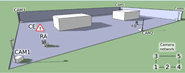
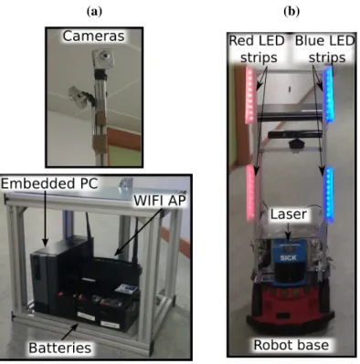
We aim at developing a system that provides a framework for the fast and easy deployment of ubiquitous robots in diverse environments. We propose a multi-agent system such as the one illustrated in Figure1, which consists of two main elements: (a) an intelligent control system formed by camera-agents spread out on the environment (CAM1 to CAM5 in the figure), and (b) autonomous robots navigating on it (RA and RB, in the figure). Each camera-agent consists of an aluminium structure like that of Figure1, which is easy to transport, deploy and pick up. This aluminium structure has two parts: A box and a mast attached to it. As it is shown in Figure2(a), the box contains a processing unit, a WiFi Access Point and power supplies, while the mast holds one or more video cameras (one for each camera-agent). Regarding the robots, we work with Pioneer 3DX robots like the one in Figure2(b). These robots are equipped with a laser scanner, sonar sensors, and a set of colour LED strips, which form patterns that can be recognized from the cameras, as we will explain in Section5.4.
Figure 1. Example of the deployment of the multi-agent system: Camera-agent 3 (CAM3) is detecting a Call Event, while robot-agent A (RA) is being sighted by camera-agent 1 (CAM1) and robot-agent B (RB) by camera 2 (CAM2).
we do not require the existence of a cable network, because the communications amongst our agents are lightweight enough to work with wireless networks.
Figure 2. (a) Camera-agent: camera-agent’s cameras (top), and camera-agent’s box with embedded PC, batteries and WiFi AP (left-bottom). (b) Robot-agent, with its laser range finder and LED strips for identification from the cameras.
(a) (b)
4. System Requirements
Once deployed, our system will detect those situations that require the assistance of our robots, and it will enable our robots to navigate towards the areas where these situations are detected. The camera network will be in charge of detecting such situations (called Call Events, or CEs like in Figure1). This will increase the range of action of our robots.
We would like to point out that the concept of Call Event can be accommodated to a wide range of situations. For example, Call Events may be triggered by users asking explicitly for assistance (e.g., by waving in front of a camera). Even more, Call Events can be activated even if no user triggers them explicitly, for instance taking into account the behaviour of the people in the environment. This is very interesting, because it would enable the robots to anticipate to the users’ needs [27]. For example, in the context of a museum tour-guide robot, our cameras could detect groups of people that are staying still at the entrance of the museum, infer that they may need assistance, and send the robot towards them. This will indeed be perceived by the users as a pro-active behaviour.
5. System Tasks
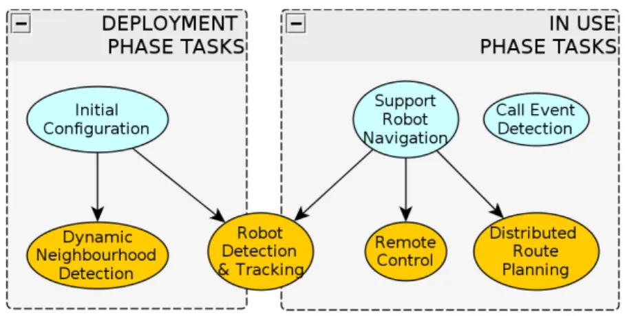
To set our system working and accomplishing the requirements described in Section 4, we need to consider two separate and important phases: the “deployment” phase and the “in use” phase. Each phase requires different tasks, represented in Figure 3. All the tasks of the system are coordinated in a self-organized manner [28]. We must bear in mind that there are several definitions of self-organization, some of which imply the existence of emergence, while some others do not [29]. We consider our system self-organized because coordination arises from local interactions among independent agents. Moreover, the system is fully distributed, since there is no hierarchy or centralization in either control or knowledge storage. However, we would like to point out that there are no emergent processes in our system.
Figure 3. Camera tasks during the deployment and in use phases.
these cameras will be always monitoring their neighbourhood relationships to account for changes in their pose.
At the “in use” phase, the cameras will be monitoring the environment in order to detect situations that require the presence of the robots (Call Event detection). Since the robots do not have maps of the environment, the cameras will plan routes through which the robot will navigate to get to the Call Events (distributed route planning), using their neighbourhood knowledge. Finally, the cameras will be responsible for supporting the movement of the robots along these navigation routes (remote control), for which they need to be able to detect and track the robots (robot detection and tracking). On the other hand, the robots’ tasks are restricted to navigating safely towards the Call Events detected from the cameras and to provide assistance. In the next subsections, we will describe all the tasks previously mentioned.
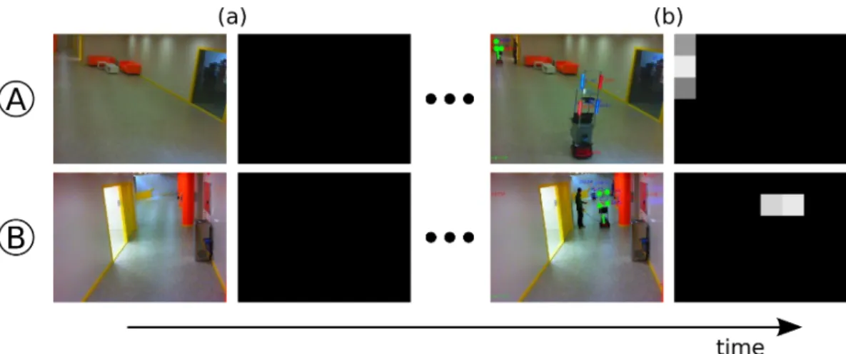
Figure 4. Evolution of the Neighbourhood Probability of two cameras A and B through time. Black represents a probability equal to zero, and white a probability equal to one. (a) Initially, the cameras assume no neighbourhood relationships. (b) Nevertheless, as the robot is moved around and the time elapses, the simultaneous detections allow the establishment of non-null neighbourhood values between both cameras.
5.1. Dynamic Neighbourhood Detection
Our system must guarantee the correct robot navigation towards the areas where their presence is required. We want to favour self-configuration over manual tuning, and avoid the use of prior knowledge of the environment where the robot will move. To this end, each camera of the system is capable of determining automatically which other cameras are its neighbours. This will enable the calculation of routes as sequences of cameras through which the robots will have to navigate to reach a specific area, as we will see in Sections5.2and5.3.
To establish neighbourhood relationships amongst them, the cameras detect parts of their FOV that overlap with the FOV of other cameras (these overlapping areas in the FOV will be called Neighbourhood Regions from now on). Specifically, each camera divides its FOV in squared regions, and calculates the Neighbourhood Probability of each region with all the remaining cameras, i.e., for a specific camerai, the Neighbourhood Probability of each region of the FOV of camera i, with respect to each camera j,
These Neighbourhood Probabilities will be computed by detecting simultaneous events from the cameras. Whenever a camera detects a robot, it stores the region where the robot was detected and broadcasts the detection of the robot to all the other cameras. Periodically, each camera checks whether the detection of the robot is taking place simultaneously with the detection of the same robot but from any other camera. When two cameras detect a robot simultaneously, they increase the Neighbourhood Probability of the region where the robot was detected. On the contrary, when this detection does not take place simultaneously, they decrease this probability. We compute all the probability updates using a Bayesian binary filter [30].
Figure4represents the evolution of the Neighbourhood Probabilities between two cameras, A and B. Initially (Figure4(a)), there were no simultaneous robot detections among them, so the Neighbourhood Probability was zero for all the regions. After a few common robot detections (Figure 4(b)), both cameras recognised their common regions with probability close to one. Therefore, they established a neighbourhood link, and tagged those regions as Neighbourhood Regions.
This dynamic neighbourhood detection is not only carried out during the “deployment” stage, but also during the “in use” phase, since the neighbourhood relationships can change dynamically (e.g., if some camera is moved or if it stops working). Therefore, the cameras are continuously updating this neighbourhood information to adapt to eventual changes.
5.2. Distributed Route Planning
A route is an ordered list of cameras through which the robot can navigate. Basically, the robot will go from the FOV of one of the cameras to the FOV of the next camera on the route, without needing metric maps of the environment. These routes will be generated as a result of local interactions amongst the cameras, without the intervention of any central agent.
Figure 5. Distributed route planning procedure. Cameras (1–5) established their neighbourhood relationships, forming a network altogether. (a) Call event detection and call for robots. (b) Back-propagation process for route formation. See Section 5.2 for a detailed explanation.
(a) (b)
It is clear after this description that the route planning does not emerge from a globally coordinated process, but from a self-organized process coming from multiple local interactions among neighbouring agents, which only handle local information.
5.3. Remote Control and Robot Navigation
A route is a sequence of cameras. Any robot following a route must traverse the FOVs of those cameras involved in it: each camera on the route helps the robot to move towards the next Neighbourhood Region, so that the robot reaches the FOV of the next camera in the route. This remote control process is illustrated in Figure6. First of all, if a camera sees a robot, it enquires the robot whether it is following a route, and if that is the case, for the sequence of cameras that form part of it. Then, the camera informs the robot about the direction that it should follow to get to the Neighbourhood Region shared with the next camera on the route. The camera will repeat this process (e.g., each few seconds) until the robot arrives at the next camera, which will continue guiding the robot by the same process, and so on. The control of the robot is purely reactive, updated with each new camera command. Unlike most proposals [10,11,23,31,32], we do not require our cameras to calculate the robot position in the world coordinates (just its orientation or movement direction), and hence we do not need to calibrate the cameras.
For the robot navigation, we use the classic but robust Potential Fields Method [33]: The robot moves towards the goal position commanded by the camera, which exerts an attractive force on it, while the obstacles detected by the laser scanner exert repulsive forces, so that the robot avoids colliding with them.
5.4. Robot Detection and Tracking
As we outline in Figure3, the robot control and navigation and the dynamic neighbourhood detection amongst the cameras depend on the robust detection and tracking of the robots. For several reasons, we propose to mount on the robots patterns of light emitting markers (active markers) that are easy to recognize from the cameras. First of all, according to our experience, it is not possible to extract reliable features at the distances that we want our system to work (up to 20 or 30 meters), neither from the robot itself nor from passive markers mounted on it. On the other hand, we require our system to work in various illumination conditions, which can range from over illuminated spots to semi-dark places. In our experiments, we observed that neither the robot natural features nor passive markers were robust enough to cope with this (similar problems were reported by [32,34]). Moreover, regarding the task of rigid object tracking, using artificial markers tends to provide higher accuracy rates than the use of natural features [35]. Finally, the use of markers of different colours enables our system to differ among multiple robots, and thus increases the scalability of the system. Hence, we assume that the use of active markers of different colours is a very reasonable solution for our problem.
in our experience, the users find the light of high illumination active markers unpleasant. We also considered the use of IR LEDs [15], but their performance is very bad under natural illumination.
Figure 7. Robot detection and tracking algorithm. Continuous arrows indicate flow of execution. Dashed arrows indicate influence relationships. Dotted arrows indicate data input/output.
We would like to point out that our algorithm allows us to use more than one robot simultaneously: It is sufficient that each robot carries a marker with a different colour pattern (see the experiment in Section 6.2). However, for the sake of clarity, we will describe the algorithm with the example of the detection and tracking of a single robot that carries the marker shown in Figure2(b).
5.4.1. Stage 1: Blob Detection and Tracking
Figure8shows the blob detection and tracking stage of our algorithm. In our context, a blob is a set of connected pixels of the same colour. The first step of this stage (step A, Figure8) filters out the pixels whose colour does not match up with any of the colours of the LED strips (red and blue in this case, as in Figure 2(b)). Two kinds of pixels, and therefore blobs, will pass this filtering process: the robot blobs, and spurious blobs (pixels that match the colours of the LED strips, but are due to artificial lights, reflections of the light coming out from the robot active markers,etc.).
After this filtering, we assign a Kalman Filter to each blob (step B, Figure8). Thus, we can assign an identity to each blob and track it over consecutive frames (B1, B2, B3,etc., in Figure8).
Figure 8. Stage 1: Blob detection and tracking.
5.4.2. Stage 2: Robot’s marker recognition
In this stage, represented in Figure 9, we identify the groups of blobs that may correspond to the robot’s marker LED strips. For example, in Figure 8, these blobs would be B6, B7, B8, and B9. To do this, we carry out the three stage process described in the next subsections, aimed to calculate the degree of similarity (likelihood) between each group of detected blobs and the robot marker.
Shape Analysis of Each Blob
First of all, we evaluate whether or not the aspect ratio (height-width ratio) of each blob is approximately equal to the aspect ratio of the LED strips of the marker (this value is six in our case). From this evaluation, we assign a likelihood to each individual blob, and only those with a non-zero likelihood will be considered in the next step (eligible blobs).
Pattern Construction and Matching
can construct groups ofeligible blobs, calculate their respective colour patterns (step D, Figure9), and match them against the known colour pattern of the group of LEDs (step E, Figure9). To this extent, we have chosen a pattern representation that captures (a) the blobs that form the pattern, (b) their colours, and (c) their geometrical disposition (chain codes).
Figure 9. Stage 2: Robot’s Marker Recognition.
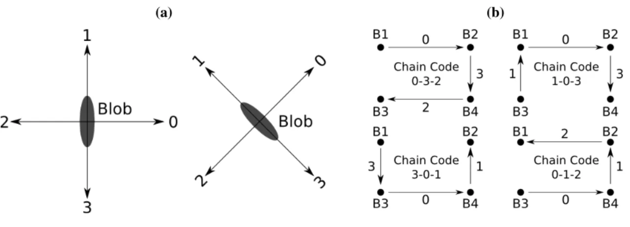
not to the image coordinates (Figure 10(a)): This makes our chain codes invariant to rotations lower than±90◦. Clearly, the points of Figure10(b) accept several representations, depending on the election of the initial blob and on the rotation sense of the displacements (clockwise or counter-clockwise): 0-3-2, 3-0-1, 1-0-3, 0-1-2,etc.
Figure 10. (a) Displacement codes of the chain code. We calculate the displacements with respect to the blob coordinates: invariance on rotations lower than ±90◦. (b) Examples of chain codes of a set of four points. Not all possible chain codes are included.
(a) (b)
At this point, we are able to construct the pattern of each group of blobs, based on the properties previously described. For instance, to construct the marker model patterns (Figure9), we start calculating all the possible sequences of 2, 3, and 4 blobs of the model (B1-B2, B1-B2-B3, B1-B2-B3-B4, etc.). Then, we calculate the chain code of each sequence. For example, the sequence B1-B2-B4-B3 would be associated with the chain code 0-3-2. Finally, we construct the sequence of colours of the blob sequence. In the same example, since B1 and B3 are red, and B2 and B4 are blue, the colours for B1-B2-B4-B3 will be R-B-B-R. This codification may seem redundant, but we are just codifying all the possible colours and geometrical dispositions of the blobs, in the absence of a mechanism to identify them univocally.
We follow a similar process to construct the patterns that form the groups of eligible blobs (step D, Figure 9). In the following, we match these patterns (detected patterns in Figure 9) with the marker model patterns (step E, Figure 9). This matching process results in a list of selected patterns, which contains the patterns that form the robot groups and coincide with any of the robot marker model patterns.
Geometry Analysis of Each Pattern
each individual blob (from the eligible blobs list, Figure9). To calculate the likelihood of each pair of blobs, we measure the degree of compliance with the following criteria:
1. The blobs must be similar in height, width, and orientation with respect to the horizontal axis (represented asH,W andθin Figure11(a), respectively).
2. The blobs must respect certain distances among them. If the blobs are collinear (up or down displacement, like among blobs 1 and 2 in Figure 11(a)), the distance in x (Dx in Figure 11(a))
must be approximately zero, and the distance in y (Dy in Figure 11(a)) approximately twice the
height of one of the blobs. On the contrary, if the blobs are not collinear (left or right displacement, like among blobs 1 and 3 in Figure 11(a)), Dy must be approximately zero, and Dx less or
approximately equal to the height of one of the blobs.
Like in the case of the chain codes (Figure 10), all the criteria are calculated with respect to the coordinates of the blob, not with respect to the coordinates of the image (except for the blob’s orientation). Hence, this likelihood measurement will be invariant to rotations.
Figure 11. (a) Geometric properties taken into account in the pattern matching process: Blob width W, height H, and angle with respect to the horizontal axis θ, to measure parallelism among blobs, and horizontal (Dx) and vertical (Dy) distance among blobs. (b)
Robot position and orientation estimation.
(a) (b)
5.4.3. Stage 3: Robot Detection
to the robot that carries the marker, our algorithm discards those that do not persist over a minimum time interval (persistence time interval). Next, the algorithm calculates the average likelihood over the mentioned interval of the remaining blob groups. The persistence time interval was introduced to increase the robustness of the algorithm against spurious noises: Reflections of the marker or ambient lights, objects moving around, spurious noise that passes the colour filter, etc. While the robot blob groups are usually stable (high average likelihood rates over long time intervals), noise blobs are rather erratic in persistence, shape, and position (possible instantaneous likelihood peaks, but low average likelihood rates in general). On the other hand, this interval smoothens the impact of momentary drops on the likelihood of the robot blob groups.
At this point, the algorithm is able to decide whether there is a robot present in the camera images. The decision process varies depending on whether the algorithm has previously detected a robot or not. In case that the robot was detected in the previous iteration, the algorithm checks if its previously detected blob group exists in the current list of eligible patterns. If that is the case, the algorithm selects the same blob group as in the previous iteration, provided that its likelihood is higher than zero. It may also occur that some of the blobs of this group do not exist anymore. In this case, the algorithm selects the eligible pattern with the highest number of blobs in common with the group selected in the previous iteration. In following iterations, the algorithm will seek to extend this group with new blobs, to recover from the loss of the missing blobs. This ensures the stability of the robot tracking and its robustness against temporary occlusions. On the other hand, if the detected blob group detected in previous iterations disappears completely, or if the robot was not detected in the previous iteration, the algorithm simply selects the eligible pattern with the highest number of blobs. In case of a tie among two or more groups, the algorithm selects the one with the highest average likelihood over the persistence time interval.
5.4.4. Stage 4: Pose Estimation
The last stage of the algorithm calculates the pose of the robot (step I, Figure7). The robot position is calculated by projecting the centre of masses of its blobs onto the ground plane (star in Figure11(b)). We know the real dimensions of the LED lights and their height with respect to the ground, so the projection is straightforward. With regard to the robot orientation, the algorithm first decides whether the robot is giving its front or its back to the camera, considering the chain code and the colours of its blobs. Then, the orientation direction, represented as an arrow in Figure 11(a), is calculated from the lines connecting parallel blobs. Although this does not give a high precision, it is more than enough for robot control, as we will show in our experimental results (Section6).
6. Implementation and Experimental Results
was implemented using the Player(v-3.0.2)-Stage(v.4.0.0) platform, and for image processing (camera software) we used the OpenCV 2.2 library [38]. Regarding communications, messages were passed over an IEEE 802.11g local wireless network via UDP.
Figure 12. (a) Camera network deployed in the experiments. Each camera is represented by a letter (from A to G), and each FOV is represented by a coloured region. The trajectory represented is the same as in (b). (b) Robot trajectory through the route B-C-D-E-F-G (70 m long). (c) Robot trajectory through the route A-B-C-D-E (60 m long). (d) Robot trajectory through the route E-D-C-B ( 50 m long). We provide explanations of each trajectory in the text.
(a) (b)
(c) (d)
We deployed the multi-agent system shown in Figure12(a), which consists of seven camera-agents (A to G) and a robot-agent (R). Each camera covered one corridor, and each had two neighbours at most (their FOVs can be seen both in Figures 12 and 13). For instance, cameras B and C covered two perpendicular corridors, being A and C the neighbours of B, and B and D the neighbours of C. Note that this is not the only distribution that our system allows (e.g., cameras may have more than two neighbours), but the most natural one given the topology of the environment. After the deployment of the system, the cameras recognised their camera neighbours correctly. This completed the validation of the dynamic neighbourhood detection task (Section5.1).
Finally, the robot moved through this route supported by the cameras. We show three of the most representative robot trajectories from these experiments in Figure 12(b,c,d). In all the experiments, the robot moved at the maximum possible speed considering its weight (0.5m/s). As an example, in Figure14we show the linear speed of the robot during the trajectory in Figure12(c). The speed of the robot varies depending upon the environment and the camera commands. We obtained all these data from the robot’s odometry and laser logs using the PMAP SLAM library, compatible with Player-Stage. The maps and trajectories were obtained off-line just for visualization purposes: As we have explained before, our system does not need maps of the environment.
Figure 13. Example of camera captures from the experiment in Figure 12(c): (a) camera A, (b) camera C, (c) camera D, (d) camera E. The detected marker is rounded by a convex polygon, and each of its blobs is tagged with a circle.
(a) (b)
(c) (d)
In the second experiment (Figure 12(c)) camera D sighted the call event, and the robot navigated through the route A-B-C-E-D, starting from camera A. The trajectory was 60 m long, and as in the previous experiment, the result was satisfactory. Figure14represents the linear speed of the robot during this trajectory.
In both experiments, the robot movement was counter-clockwise. In the last experiment (Figure 12(d)), we tested a clockwise movement. In this case, camera B detected the call event, and the robot moved towards it through the route E-D-C-B, starting from camera E. The trajectory length was 50 m long approximately. Although the trajectories were satisfactory, we observed two kinds of
Figure 14. Linear speed of the robot during the experiment represented in Figure12(c).
do not cover. This would allow us to eliminate the need of FOV overlap among neighbouring cameras (Section5.1). In this sense, we are already analysing the performance of different systems on this task [26].
We have performed many of these experiments varying the initial position of the robot and of the call event. The system proved to be robust, because the robot always arrived within a circle of 2 m around the call event area. We believe that this is sufficient for most real world applications where our system could be used. For example, this would suffice if the robot is meant to approach groups of people to offer them information, or to navigate towards areas where an anomaly is detected. On the other hand, in all the experiments that we have carried out, the success of the robot was 100%. This success rate depends on the number of the cameras and the dimensions of the space they cover. For this reason, in the next section we perform a careful analysis of the maximum recommended working range of each camera, and some other aspects that are relevant to guarantee such a high success rate. In future works, we plan to measure how this success rate varies according to factors such as the number of the people in the environment, the length of the trajectory,etc.
6.1. Robot Detection and Tracking
The robot detection and tracking algorithm is a critical part of the system, and has been explained thoroughly in Section5.4. We have considered it appropriate to undertake a quantitative analysis of its performance, which we detail in this section. To this extent, we have constructed a dataset from the video recorded by each of the five cameras of the experiment in Figure13(c). In this experiment, camera B recorded the robot at a distance up to 4 m (approximately), E up to 15 m, A and C up to 30 m, and D up to 50 m. The cameras recorded video at 15 fps during 14 minutes, making a total of 12564 frames in our dataset.
We have executed our algorithm on this dataset with different parameter variations to test their impact on the performance of the algorithm. Particularly, we have considered variations on:
• Colour Filters. To detect the marker of the robot, we need to detect its colours first (see Section 5.4.1). We define each colour that has to be detected as an interval in the HSV colour space. To detect the colours of the marker, we filter out every pixel whose colour is out of the desired intervals. We observed that the illumination conditions affect the S and V colour components very strongly, thus their corresponding intervals have to be adjusted for each environment. A careful adjustment is prohibitive if we want to deploy our robots quickly, but a coarse one may let undesired colours pass the filtering stage. For these reasons, we assessed the performance of the algorithm with two colour filters: (1) one with carefully adjusted intervals, and (2) another with coarsely adjusted intervals.
For each frame, our algorithm tells us whether it detected the robot, and if that is the case, its position. To analyse the results, we classified each frame into one of the following five classes (confusion matrix in Table1):
• True Positive (T P): If there was a robot in the scene and the camera detected it. The higher the better.
• False Positive—Robot in Scene(F PRS): If there was a robot in the scene and the camera detected
another element. The lower the better.
• False Negative(F N): If there was a robot in the scene and the camera did not detect it. The lower the better.
• False Positive—No Robot in Scene (F PN RS): If there was no robot in the scene but the camera
detected one. The lower the better.
• True Negative (T N): If there was no robot in the scene and the camera did not detect any robot. The higher the better.
We divided the False Positives in two different groups to have a separate measure of the noise caused by the markers’ lights reflections (which commonly causes the F PRS rate) from the rest of the noise
(which commonly causes theF PN RSrate).
Table 1. Confusion matrix used to classify the robot detection and tracking algorithm results.
Is there a robot?
Yes No
Detects
Robot
The robot is the same as the real robot T P
F PN RS
The robot is different than the real robot F PRS
Nothing F N T N
According to our experience, the accuracy of the remote control of the robot from the cameras drops significantly at distances higher than 20 or 30 m. Moreover, at this distance, the marker is too small to be detected accurately. Therefore, we usually restrict the effective coverage of the cameras to distances below this range. For this reason, to analyse the results, we considered two different levels of requirement regarding the maximum distance at which our algorithm must detect the robot: (1) arbitrarily large distances, and (2) distances below 20 m. We are mostly interested in this last case.
column, we see that the averageT P and F N rates are not ideal, but acceptable for our purposes: If a camera fails to detect a robot occasionally, our system will still be able to support the robot navigation, because the acquisition rate of each camera is high with respect to the speed of the robot. In fact, it is enough if the cameras are able to detect and send a command to the robot every few seconds. On the other hand, we observe that the results of the algorithm are the best when we use carefully adjusted colour filters. However, to tune them in every camera at deployment time would be prohibitive. Fortunately, we also observe that we obtain similar results if we use a persistence time interval of 10 frames, even with coarsely adjusted colour filters. Specifically, this improves the F P andT N rates, which are the most important for us. Therefore, we can adjust the colours filters coarsely, which can be done very quickly, and still achieve a great robustness on the detection and tracking of the robot. Finally, as it was expected, the overall results of the algorithm improve when we do not require the algorithm to detect the robot at distances greater than 20 m. The most typical scenario in real deployments (like experiments in Section6) is remarked in boldface.
Table 2. Classification results of the detection and tracking algorithm. We have analysed eight different scenarios by varying: MaxDist (maximum distance at which we require the cameras to detect the robot), ColFilt (whether the colour filters have been coarsely or carefully adjusted), and Int (time persistence interval). The typical configuration that we use on robot control experiments (like those on Section 6) is remarked in boldface. The acronyms are: TP(True Positives),TN (True Negatives),FP-RS(False Positive—Robot in Scene),FP-NRS(False Positive—Not Robot in Scene),FN(False Negatives),PPV(Positive Predictive Value or Precision), Negative Predictive Value (NPV),TPR(True Positive Rate or Recall),MCC(Matthews Correlation Coefficient).
MaxDist =∞ MaxDist =20m
ColFilt = Coarse ColFilt = Careful ColFilt = Coarse ColFilt = Careful
Int =0 Int =10 Int =0 Int =10 Int =0 Int =10 Int =0 Int =10 Avg T P 0.528 0.451 0.609 0.516 0.760 0.614 0.872 0.764 0.639 T N 0.958 0.999 1.000 1.000 0.946 0.999 1.000 1.000 0.988 F PRS 0.238 0.007 0.018 0.006 0.132 0.003 0.028 0.009 0.055
F PN RS 0.042 0.001 0.000 0.000 0.054 0.001 0.000 0.000 0.012
F N 0.234 0.543 0.373 0.479 0.108 0.383 0.101 0.228 0.306
P P V 0.627 0.983 0.971 0.989 0.725 0.992 0.969 0.989 0.906 N P V 0.881 0.769 0.829 0.790 0.962 0.893 0.966 0.926 0.877 T P R 0.693 0.454 0.620 0.519 0.876 0.616 0.897 0.770 0.680 M CC 0.485 0.632 0.700 0.666 0.713 0.717 0.879 0.804 0.699
the Matthews Correlation Coefficient (M CC) ranges in [–1, 1] (−1 representing an inverse prediction, 0 an average random prediction and +1 a perfect prediction).
P P V = T P
For the reasons already mentioned, the robot control problem requires to maximize the P P V rate (proportion of frames where the robot is detected and the detection is correct), and maintain to an acceptable rate the N P V (proportion of frames where the robot is not detected and there is no robot) and theT P Rvalues (proportion of frames where there is a robot and is correctly detected). The results in Table2confirm that our algorithm is very well suited to this problem. Moreover, the M CC values, which measure the quality of the classifications, confirm the good performance of the proposed classifier. Summarizing, we conclude that our algorithm is very robust to be used in the context of robot control. We have also observed that the use of the persistence time interval ensures the robustness of the algorithm even with coarsely adjusted colour filters. This guarantees that we will be able to deploy our system in different environments in a fast and easy manner. Considering these results, we think that it is important to highlight that in all the experiments of Section 6 we have used the same colour filters (coarsely adjusted), for all the cameras, and regardless of the illumination conditions.
6.2. Scalability with the Number of Robots
The architecture of our system allows the management of multiple robots naturally. Each agent has a unique ID, which allows it to communicate and coordinate with the rest of agents. Obviously, the cameras must identify each robot univocally to assign it an ID, so our robots carry active markers with unique colour patterns. Considering this, the weakest part of our system concerning scalability lies in the proper identification of each robot from the cameras.
We have performed an experiment to test our robot detection and tracking algorithm with more than one robot. To this extent, we have deployed four cameras, and we moved two robots around (Figure15(a)). Figure15(b) shows both robots seen from one of the cameras.
Table3shows the results of the experiment. On the one hand, theT P,T N,F PRS,F PN RS, andF N
Figure 15. Deployment of our self-organised multi-agent network with two robots working in the environment. (a) FOV of each camera, and trajectory of one of the robots. (b) Snapshot of both robots taken from camera C.
(a) (b)
Table 3. Classification results of the detection and tracking algorithm with two robots. M ISCL(misclassification rate) is the percentage of frames where the algorithm confuses one robot with the other. The rest of the acronyms have been defined in Section6.1.
T P T N F PRS F PN RS F N M ISCL
Robot1 0.781 0.995 0.031 0.005 0.18 0.004 Robot2 0.821 0.996 0.283 0.004 0.151 0.009
Table 4. Execution times of the robot detection and tracking algorithm. µ is the average processing time per image (in milliseconds), and σ is the standard deviation (in milliseconds). NumRobots refers to the number of different robots that the algorithm tries to detect. NumCams refers to the number of camera-agents executed on a single computer (concurrently).
NumRobots = 1 NumRobots = 2
NumCams = 1 NumCams = 2 NumCams = 1 NumCams = 2
Cam1 Cam1 Cam2 Cam1 Cam1 Cam2
µ(ms) 15.66 16.60 16.31 32.57 32.63 32.57 σ(ms) 1.37 1.49 1.67 3.27 3.24 3.27
more than one camera concurrently, as expected of a multi-core processor. Finally, the processing time scales linearly with the number of robots to be detected, each robot increasing this time in16ms (e.g., 2 robots require32ms). We would like to point out that the current processing time is good enough for our requirements, but there is still a lot of room for improvement: code optimization, parallelization, use of GPU, etc. For example, right now each camera computes the detection of all the robots in the same CPU core, but it could instead compute the detection of each robot in a different core.
All in all, our system is able to handle more than one robot, because: (1) the software architecture allows it, (2) the cameras can identify each robot univocally, and (3) in the worst case, the computational time required scales linearly with the number of robots.
7. Summary, Conclusions, and Future Work
In this paper, we described a robotic system intended to deal with two problems that are preventing cutting edge service robots to work out of the research centres: The cost of their deployment in new environments, and the poor perception of the users on the quality of their services. On the one hand, to be cost-effective, the deployment of the robotic systems should be automatic, fast and easy, but in practice it usually requires several days of adaptation to the environment conditions. On the other hand, the perception of the users on the quality of the robot services is tightly related to the ability of the robots to perceive their needs and to show initiative to attend them, regardless of where they happen in the environment. To tackle these problems, we have combined robotics, ambient intelligence and ubiquitous computing technologies to propose a system fast and easy to deploy, which enables our robots to perceive and attend users’ needs anywhere in the environment.
Our system consists of a distributed multi-agent network formed by two kinds of agents: intelligent cameras that can be easily spread out on the environment, and autonomous robots navigating in it. Each camera can discover its camera neighbours by detecting simultaneous events in their Field of View. This is a self-organized and decentralized process that automatizes the deployment and speeds up the start-up of the system. The cameras serve two main purposes. On one side, they detect situations that require the presence of the robots. This increases the range of perception of the robots and enhances the opinion of the people on their pro-activity. On the other, the cameras support the robot navigation in absence of a map of the environment. This is done by means of two self-organized processes: (1) the cameras calculate the routes of cameras through which the robot can move, and (2) each camera helps the robot to get to the next camera on the route. All of this results in a robust, flexible and scalable system.
We demonstrated in real world experiments that our robots are able to attend to events detected by the cameras, regardless of the positions of the robots and the events. Given its importance for the performance of our system, we have also proposed a method for the detection and tracking of our robots. Experimental results showed its robustness in the context of robot control, even in the presence of noise and under different illumination conditions.
we are working on the recognition of scenes that require the presence of our robots: groups of people standing still for long periods of time, people waving at the cameras,etc.
Acknowledgements
This work was supported by the research projects TIN2009-07737, INCITE08PXIB262202PR, and TIN2012-32262, the grant BES-2010-040813 FPI-MICINN, and by the grant “Consolidation of Competitive Research Groups, Xunta de Galicia ref. 2010/6”.
References
1. International Federation of Robotics Statistical Department, World Robotics 2011; VDMA Robotics + Automation: Frankfurt, Germany, 2011.
2. Kim, J.; Lee, K.; Kim, Y.; Kuppuswamy, N.; Jo, J. Ubiquitous Robot: A New Paradigm for Integrated Services. In Proceedings of the IEEE International Conference on Robotics and Automation, Roma, Italy, 10–14 April 2007; pp. 2853–2858.
3. Buhmann, J.; Burgard, W.; Cremers, A.; Fox, D.; Hofmann, T.; Schneider, F.; Strikos, J.; Thrun, S. The mobile robot rhino. AI Magazine1995,16, 31–38.
4. Thrun, S.; Bennewitz, M.; Burgard, W.; Cremers, A.; Dellaert, F.; Fox, D.; Hahnel, D.; Rosenberg, C.; Roy, N.; Schulte, J. MINERVA: A Second-Generation Museum Tour-Guide Robot. In Proceedings of the IEEE International Conference on Robotics and Automation, Detroit, MI, USA, 10–15 May 1999; pp. 1999–2005.
5. Siegwart, R.; Arras, K.; Bouabdallah, S.; Burnier, D.; Froidevaux, G.; Greppin, X.; Jensen, B.; Lorotte, A.; Mayor, L.; Meisser, M.; et al. Robox at Expo.02: A large-scale installation of personal robots. Robot. Auton. Syst. 2003,42, 203–222.
6. Trahanias, P.; Burgard, W.; Argyros, A.; Hahnel, D.; Baltzakis, H.; Pfaff, P.; Stachniss, C. TOURBOT and WebFAIR: Web-Operated mobile robots for tele-presence in populated exhibitions. IEEE Robot. Autom. Mag.2005,12, 77–89.
7. Rodriguez-Losada, D.; Matia, F.; Galan, R.; Hernando, M.; Montero, J.; Lucas, J. Urbano, an interactive mobile tour-guide robot. In Advances in Service Robotics; Seok Ahn, H., Ed.; InTech: Rijeka, Croatia, 2008; pp. 229–252.
8. Lee, J.; Hashimoto, H. Intelligent space concept and contents. Adv. Robot.2002,16, 265–280. 9. Lee, J.; Morioka, K.; Ando, N.; Hashimoto, H. Cooperation of distributed intelligent sensors in
intelligent environment. IEEE/ASME Trans. Mechatron. 2004,9, 535–543.
10. Lee, J.; Hashimoto, H. Controlling mobile robots in distributed intelligent sensor network. IEEE Trans. Ind. Electron. 2003,50, 890–902.
11. Steinhaus, P.; Strand, M.; Dillmann, R. Autonomous robot navigation in human-centered environments based on 3D data fusion. EURASIP J. Appl. Signal Process. 2007, doi:10.1155/2007/86831.
13. Pizarro, D.; Mazo, M.; Santiso, E.; Marron, M.; Jimenez, D.; Cobreces, S.; Losada, C. Localization of mobile robots using odometry and an external vision sensor. Sensors 2010, 10, 3655–3680.
14. Losada, C.; Mazo, M.; Palazuelos, S.; Pizarro, D.; Marr´on, M. Multi-Camera sensor system for 3D segmentation and localization of multiple mobile robots. Sensors2010,10, 3261–3279. 15. Fern´andez, I.; Mazo, M.; L´azaro, J.; Pizarro, D.; Santiso, E.; Mart´ın, P.; Losada, C. Guidance of
a mobile robot using an array of static cameras located in the environment. Auton. Robots2007, 23, 305–324.
16. Saffiotti, A.; Broxvall, M. PEIS Ecologies: Ambient Intelligence Meets Autonomous Robotics. In Proceedings of the 2005 Joint Conference on Smart Objects and Ambient Intelligence: Innovative Context-Aware Services: Usages and Technologies, Grenoble, France, 12–14 October 2005; pp. 277–281.
17. Saffiotti, A.; Broxvall, M.; Gritti, M.; LeBlanc, K.; Lundh, R.; Rashid, J.; Seo, B.; Cho, Y. The PEIS-Ecology Project: Vision and Results. In Proceedings of the IEEE/RSJ International Conference on Intelligent Robots and Systems, Nice, France, 22–26 September 2008; pp. 2329–2335.
18. Lundh, R.; Karlsson, L.; Saffiotti, A. Autonomous functional configuration of a network robot system. Robot. Auton. Syst.2008,56, 819–830.
19. Shiomi, M.; Kanda, T.; Ishiguro, H.; Hagita, N. Interactive Humanoid Robots for a Science Museum. In Proceedings of the 1st ACM SIGCHI/SIGART Conference on Human-Robot Interaction, Salt Lake City, UT, USA, 2–4 March 2006; pp. 305–312.
20. Shiomi, M.; Kanda, T.; Glas, D.; Satake, S.; Ishiguro, H.; Hagita, N. Field Trial of Networked Social Robots in a Shopping Mall. InProceedings of the IEEE/RSJ International Conference on Intelligent Robots and Systems, St. Louis, MO, USA, 10–15 October 2009; pp. 2846–2853. 21. Shiomi, M.; Sakamoto, D.; Kanda, T.; Ishi, C.; Ishiguro, H.; Hagita, N. Field trial of a networked
robot at a train station. Int. J. Soc. Robot.2011,3, 27–40.
22. Sanfeliu, A.; Andrade-Cetto, J. Ubiquitous Networking Robotics in Urban Settings. In Proceedings of the IEEE/RSJ IROS Workshop on Network Robot Systems, Beijing, China, 9–15 October 2006.
23. Sanfeliu, A.; Andrade-Cetto, J.; Barbosa, M.; Bowden, R.; Capit´an, J.; Corominas, A.; Gilbert, A.; Illingworth, J.; Merino, L.; Mirats, J. Decentralized sensor fusion for ubiquitous networking robotics in urban areas. Sensors2010,10, 2274–2314.
24. Barbosa, M.; Bernardino, A.; Figueira, D.; Gaspar, J.; Gonc¸alves, N.; Lima, P.; Moreno, P.; Pahliani, A.; Santos-Victor, J.; Spaan, M.; et al. ISRobotNet: A testbed for sensor and robot network systems. IROS2009, doi:10.1109/IROS.2009.5354231.
25. Sanfeliu, A.; Hagita, N.; Saffiotti, A. Network robot systems. Robot. Auton. Syst. 2008, 56, 793–797.
27. Kanda, T.; Glas, D.; Shiomi, M.; Ishiguro, H.; Hagita, N. Who will be the Customer?: A Social Robot that Anticipates People’s Behavior from Their Trajectories. InProceedings of the 10th International Conference on Ubiquitous Computing, Seoul, Korea, 21–24 September 2008; pp. 380–389.
28. Canedo-Rodriguez, A.; Iglesias, R.; Regueiro, C.; Alvarez-Santos, V.; Pardo, X. Self-organized multi-agent system for robot deployment in unknown environments. Lect. Note. Comput. Sci. 2011,6686, 165–174.
29. De Wolf, T.; Holvoet, T. Emergence versus self-organisation: Different concepts but promising when combined. Lect. Note. Comput. Sci. 2005,3464, 77–91.
30. Thrun, S.; Burgard, W.; Fox, D. Probabilistic Robotics; MIT Press: Cambridge, MA, USA, 2005.
31. Rekleitis, I.; Meger, D.; Dudek, G. Simultaneous planning, localization, and mapping in a camera sensor network. Robot. Auton. Syst. 2006,54, 921–932.
32. Cassinis, R.; Tampalini, F. AMIRoLoS an active marker internet-based robot localization system. Robot. Auton. Syst. 2007,55, 306–315.
33. Choset, H.; Lynch, K.; Hutchinson, S.; Kantor, G.; Burgard, W.; Kavraki, L.; Thrun, S.Principles of Robot Motion: Theory, Algorithms, and Implementation; MIT Press: Cambridge, MA, USA, 2005; pp. 77–85.
34. Mayer, G.; Utz, H.; Kraetzschmar, G. Playing robot soccer under natural light: A case study. Lect. Note. Comput. Sci. 2004,3020, 238–249.
35. Lepetit, V.; Fua, P. Monocular Model-Based 3D Tracking of Rigid Objects; Now Publishers Inc.: Hanover, MA, USA, 2005; pp. 1–89.
36. Kim, D.; Choi, J.; Park, M. Detection of Multi-Active Markers and Pose for Formation Control. In Proceedings of the 2010 International Conference on Control Automation and Systems, Gyeonggi-do, Korea, 27–30 October 2010; pp. 943–946.
37. Freeman, H. On the encoding of arbitrary geometric configurations. IRE Trans. Electron. Comput. 1961,EC-10, 260–268.
38. Bradski, G.; Kaehler, A. Learning OpenCV: Computer vision with the OpenCV library; O’Reilly Media: Sebastopol, CA, USA, 2008.
39. Baldi, P.; Brunak, S.; Chauvin, Y.; Andersen, C.A.F.; Nielsen, H. Assessing the accuracy of prediction algorithms for classification: An overview. Bioinformatics2000,16, 412–424.
40. Makris, D.; Ellis, T.; Black, J. Bridging the Gaps between Cameras. InProceedings of the IEEE Computer Society Conference on Computer Vision and Pattern Recognition, Washington, DC, USA, 27 June–2 July 2004; pp. II-205–II-210.
41. Ben Shitrit, H.; Berclaz, J.; Fleuret, F.; Fua, P. Tracking Multiple People under Global Appearance Constraints. In Proceedings of the IEEE International Conference on Computer Vision, Barcelona, Spain, 6–13 November 2011; pp. 137–144.
c