YOUNG STELLAR CLUSTERS CONTAINING MASSIVE YOUNG STELLAR OBJECTS IN THE VVV SURVEY

YOUNG STELLAR CLUSTERS CONTAINING MASSIVE YOUNG

Instituto de Física y Astronomía, Universidad de Valparaíso, Av. Gran Bretaña 1111, Playa Ancha, Casilla 5030, Chile;[email protected] 2

Millennium Institute of Astrophysics(MAS), Santiago, Chile

3_{Instituto de Astrofísica, Facultad de Física, Pontificia Universidad Católica de Chile, Casilla 306, Santiago 22, Chile} 4

Centre for Astrophysics Research, Science and Technology Research Institute, University of Hertfordshire, Hatfield AL10 9AB, UK 5

Gemini Observatory, Northern Operations Center, 670 N. A’ohoku Place, Hilo, HI 96720, USA 6

Departamento de Ciencias Físicas, Universidad Andres Bello, Republica 220, Santiago, Chile 7

Vatican Observatory, V00120 Vatican City State, Italy 8

Max-Planck-Institute for Astronomy, Germany

Received 2015 May 23; revised 2016 June 7; accepted 2016 June 17; published 2016 September 6

ABSTRACT

The purpose of this research is to study the connections of the global properties of eight young stellar clusters projected in the Vista Variables in the Via Lactea (VVV)ESO Large Public Survey disk area and their young stellar object (YSO) populations. The analysis is based on the combination of spectroscopic parallax-based reddening and distance determinations with main-sequence and pre-main-sequence ishochronefitting to determine the basic parameters(reddening, age, distance)of the sample clusters. The lower mass limit estimations show that all clusters are low or intermediate mass(between 110 and 1800Me), the slopeΓof the obtained present-day mass functions of the clusters is close to the Kroupa initial mass function. The YSOs in the cluster’s surroundingfields are classified using low resolution spectra, spectral energy distribution fits with theoretical predictions, and variability, taking advantage of multi-epoch VVV observations. All spectroscopically confirmed YSOs(except one)are found to be massive(more than 8Me). Using VVV and GLIMPSE color–color cuts we have selected a large number of new YSO candidates, which are checked for variability and 57% are found to show at least low-amplitude variations. In few cases it was possible to distinguish between YSO and AGB classifications on the basis of light curves.

Key words:infrared: stars–open clusters and associations: individual (VVV CL010, VVV CL012, VVV CL013,

VVV CL059, [DBS20,[DBS2003]93,[DBS2003]100,[DBS2003]130)– stars: pre-main sequence– stars: variables: general

1. INTRODUCTION

The Vista Variables in the Vía Láctea(VVV)Survey is one of the six ESO Public Surveys using the 4 m VISTA telescope (Arnaboldi et al. 2007), which scans the Galactic Bulge and southern Disk using five near-IR (NIR) filters (Minniti et al. 2010; Saito et al. 2010, 2012). The VVV data are publicly available through the VISTA Science Archive (VSA; Cross et al. 2012). Technical information about the survey can be found in Saito et al.(2012)and Soto et al.(2013). A primary goal of the VVV is to describe the numerous star clusters in its coverage area in detail, which is made possible by the infrared nature of the VVV survey, its small pixel size, and its depth, which reduce the influence of dust absorption and nebulosity in the crowded regions of the Galactic Plane. In Borissova et al. (2011), we presented a catalog of 96 new cluster candidates in the disk area covered by the VVV survey. In Chené et al. (2012) we described the methodology employed to establish cluster parameters by analyzing four known young clusters: Danks 1, Danks 2, RCW 79, and [DBS2003]132. In Chené et al.(2013,2015)we presented thefirst study of seven clusters from the Borissova et al.(2011)catalog, which contains at least one newly discovered Wolf–Rayet(WR)star member of these clusters. Later, we used the radiative transfer code CMFGEN to analyze the K-band spectra of these stars and to derive the stellar parameters and surface abundances for a subset of them (Hervé et al. 2016). In Ramírez Alegría et al. (2014) we

presented the physical characterization of VVV CL086, a new massive cluster, found at the far end of the Milky Way bar at a distance of 11±6 kpc, andfinally in Borissova et al.(2014) we reported the results of our search for new star cluster candidates projected on the inner disk and bulge area covered by the VVV survey.

In this paper we continue our analysis of star clusters using the VVV database. We present eight Galactic young clusters, which contain young stellar objects(YSOs)and/or stars with emission lines in their spectra. The main goal of this investigation is to combine photometric data for the clusters with spectroscopy of individual YSOs to better determine the properties of both the clusters and the individual YSOs.

2. THE SAMPLE

Four of the clusters in our sample are selected from the Borissova et al.(2011)catalog and the rest of the clusters are selected from the Dutra et al.(2003)catalog. All of them are in the VVV disk area(Minniti et al.2010; Saito et al.2012), and theJ,H,KSNIR images are used to construct the three-color images (Figure 1) and for photometric analysis. The coordi-nates of the clusters are given in Table1. For the VVV clusters, this is the first time that their photometric and spectroscopic analysis is presented. The[DBS2003]130 was investigated by Baume et al.(2009)and anE(B−V)of 2.3 mag and an age of 1–2 Myr were determined using the combination between

The Astronomical Journal,_152:74(_23pp)_{, 2016 September doi:10.3847}/_0004-6256/₁₅₂/₃/₇₄

optical and NIR photometry. The cluster [DBS2003]93 was described as a small embedded cluster inside the GAL322.16

+00.62 HIIregion by Moisés et al.(2011), but no deep color–

magnitude diagram (CMD) was reported. The clusters

[DBS2003]75, [DBS2003]93, and [DBS2003]100 were analyzed by Kharchenko et al. (2013) using 2MASS Figure 1.VVVJHKS composite color images of VVV CL010, VVV CL012, VVV CL013, VVV CL059,[DBS2003]75, [DBS2003]93,[DBS2003]100, and [DBS2003]130. North is up, east to the left. The stars with emission lines in their spectra are marked.

Table 1

Main Parameters of The Clusters in The Sample

Name R.A. Decl. l b E J( -K) (M−m)0 Age(Myr) Mass(Me) Γ Radius′

VVV CL010a 12:11:47 −61:46:24 298.261 +0.738 2.14±0.2 14.55±1.3 2.7±1.5 (1.8±0.5)×103 −0.88±0.15 30±9 VVV CL012 12:20:14 −62:53:06 299.385 −0.228 2.0±0.3 14.1±0.7 10.0±2.5 (1.1±0.4)×102 _{−1.31±0.25 37±3}

VVV CL013 12:28:37 −62:58:24 300.343 −0.216 2.1±0.3 13.2±1.1 3.0±2.0 (1.3±0.3)×102 _{−1.33±0.08 30±3}

VVV CL059 16:05:52 −50:47:48 331.243 +1.067 3.0±0.2 15.3±1.4 20.0±3.2 (8.3±2.1)×102 _{−1.09±0.24 55±8}

[DBS2003]75 12:09:02 −63:15:54 298.184 −0.785 1.5±0.2 13.6±1.3 2.0±1.0 (8.6±1.8)×102 _{−1.00±0.12 72±3}

[DBS2003]93 15:18:37 −56:38:42 322.160 +0.629 2.6±0.3 11.6±0.9 20.0±5.0 (2.5±0.8)×102 _{−0.95±0.09 36±4}

[DBS2003]100 16:20:26 −50:54:24 332.840 −0.590 1.1±0.1 12.78±0.8 12.0±2.5 (5.2±1.1)×102 _{−1.18±0.09 80±12}

[DBS2003]130 13:11:54 −62:47:00 305.269 −0.004 2.5±0.2 13.1±1.2 3.0±1.0 (2.2±0.9)×102 −1.13±0.34 41±11

Note. a

The distances derived by different methods yield very discrepant results, thus the value reported in the table is uncertain.

Table 2

Main Parameters of the Observed Stars in the Sample

Table 3

Main Parameters of the Observed Stars in the Sample and Log of Observations

Name S70(Jy) S160(Jy) S250(Jy) S350(Jy) S500(Jy) Sp.type Mk (J–K)0 Log

(1) (15) (16) (17) (18) (19) (20) (21) (22) (23)

CL010 Obj1 K K 247.61±6.83 86.34±1.96 39.42±1.03 K K K 2012-05-05T00:33:57.1361, SofI

CL010 Obj2 K K K K K O6-8 −3.86 −0.21 2012-05-05T00:33:57.1361, SofI

CL012 Obj1 K K K K K B1-2 −2.25 −0.13 2010-05-03T23:50:21.175, SOAR

CL012 Obj2 K K K K K K K K no spectra, literature YSO cand.

CL013 Obj1 136.16±10.04 72.81±6.01 20.31±7.39 14.17±7.43 0.00±K O8-B0 −3.28 −0.21 2010-05-03T00:20:35.271, SOAR

CL013 Obj2 K K K K K Be K K 2012-05-06T03:21:08.2385, SofI

CL013 Obj3 K K K K K B2-3 V −1.66 −0.11 2012-05-06T03:21:08.2385, SofI

CL013 Obj4 K K K K K K K K no spectra, literature YSO cand.

CL059 Obj1 129.37±2.05 125.44±11.58 151.72±6.60 62.34±3.58 29.34±2.76 K K 2011-04-11T06:46:40.0196, ISAAC

CL059 Obj2 K K K K K K K K no spectra, literature YSO cand.

DBS75 Obj1 693.44±33.09 0.00: K K K O7-B0 −3.86 −0.21 2011-04-17T00:20:50.0068, SofI

DBS75 Obj2 K K K K K K K K no spectra, literature YSO cand.

DBS75 Obj3 K K K K K K K K no spectra, literature YSO cand.

DBS93 Obj1 K K K K K K K K 2011-04-15T03:35:36.6140, SofI

DBS93 Obj2 844.40±28.34 975.70: K K K K K K 2011-04-15T03:35:36.6140, SofI

DBS100 Obj1 K K K K K O4-5 −4.68 −0.21 2011-04-17T08:52:41.0839, SofI

DBS100 Obj2 K K K K K O7-8 −3.86 −0.21 2011-04-17T08:52:41.0839, SofI

DBS100 Obj3 K K K K K O6-7 −4.13 −0.21 2011-04-17T08:52:41.0839, SofI

DBS100 Obj4 K K K K K G2-3 −1.18 0.35 2011-04-17T08:52:41.0839, SofI

DBS130 Obj1 418.99±25.94 0.00: K K K K K K 2011-04-18T02:36:44.5824,SofI

DBS130 Obj2 K K K K K K K K 2011-04-18T02:36:44.5824,SofI

4

The

Astronomical

Journal,

152:74

(

23pp

)

,

2016

September

Borissov

a

e

t

photometry (which has a limiting magnitude of around 14 in theKS-band).

3. THE CMDS AND FUNDAMENTAL PARAMETERS OF THE CLUSTERS

The procedure employed for determining the fundamental cluster parameters such as age, reddening, and distance is described in Borissova et al. (2011, 2014) and Chené et al. (2012,2013). Briefly, to construct the CMD we perform point-spread function(PSF)photometry of 10×10 arcminJ,H, and KSfields surrounding the selected candidate. Each image was taken with an 80 s exposure time. We used the VVV-SkZ pipeline, which is an automatic PSF-fitting photometric pipeline for the VVV survey (Mauro et al.2013)and Dophot (Alonso-García et al. 2015). The saturated stars (usually KS

„11.5 mag, depending on the crowding) were replaced by 2MASS stars (Point Source Catalog). Since 2MASS has a

much lower angular resolution than the VVV, when replacing stars we carefully examined each cluster to avoid contamina-tion effects of crowding, using the Point Source Catalog Quality Flags given in the 2MASS catalog. To separate the

field stars from probable cluster members, we used the latest version of thefield-star decontamination algorithm of Bonatto & Bica(2010). The algorithm divides theKS,(H–KS), and(J – KS)ranges into a grid of cells. In each cell, it estimates the expected number density of cluster stars by subtracting the respective field-star number density and, summing over all cells, it obtains a total number of member stars. Grid shifts of

±1/3 of the cell size are applied in each axis. The average of these is the limit for considering a star as a possible cluster member. Only the stars with the highest survival frequencies after all tests werefinally considered as cluster members.

We have collected spectra of 16 stars(Table2)using the IR spectrograph and imaging camera SofI in the long-slit mode, Figure 2.Radial density profiles as a function of radius of the clusters in our sample. The solid line stands for the bestfit, the arrow marks the obtained radius of the cluster.

mounted on the ESO New Technology Telescope, the Infrared Spectrometer and Array Camera (ISAAC) mounted on the Very Large Telescope (VLT), and the Ohio State InfraRed Imager/Spectrometer (OSIRIS) mounted on the Southern Observatory for Astrophysical Research (SOAR) telescope.9 The instrument set-ups give resolutions of R=2200 for SofI; 3000 for ISAAC; and 3000 for OSIRIS. Total exposure times were typically 200–400 s for the brightest stars and 1200 s for the faintest. The reduction procedure for the spectra is described in Chené et al. (2012,2013). Spectral classification was performed using atlases of K-band spectra that feature spectral types stemming from optical studies (Hanson et al. 1996, 2005; Rayner et al. 2009) in concert with the spectral atlases of Martins & Coelho (2007), Crowther et al. (2006), Liermann et al. (2009), Mauerhan et al. (2011), Meyer et al. (1998), and Wallace & Hinkle (1997). The equivalent widths (EWs)were measured from the continuum-normalized spectra using the IRAF10 task splot. When the signal-to-noise ratio (S/N)was high enough, the luminosity class of the star was determined using the EW of the CO line and the Davies et al. (2007)calibration. However, for spectroscopic targets display-ing low S/N it was difficult to distinguish luminosity ClassI objects from their ClassIII counterparts. Individual extinction and distance were estimated using the spectral classifications of the objects and the intrinsic colors and luminosities cited by Martins & Plez (2006) for O type stars and by Straižys & Lazauskaitė(2009)for the rest of the spectral types(tabulated in Table 3). The uncertainties are calculated by quadratically adding the uncertainties of the photometry and the spectral classification(e.g., two subtypes).

The projected radius of the clusters in our sample is non-homogeneously determined in the literature. Based on the much deeper VVV CMDs with respect to the previous studies, we determine the visual radius of the clusters by performing direct star counting in the KS-band with a 10″ space radius, assuming spherical symmetry. That number is then divided by the area of the rings to determine the stellar density. The projected star number density as a function of radius is shown in Figure2. The cluster boundary was determined byfitting the Elson et al. (1987) theoretical profile, which represents the young clusters well. The obtained values are tabulated in Table1, where the errors are errors from thefit.

3.1. VVV CL010

VVV CL010 was selected from the star cluster list of Borissova et al. (2011), where it is described as a reddened stellar group, superposed on the strong nebulosity of the HII

region GAL 298.26+00.74. The region contains several infrared, maser, and millimeter sources, summarized in the recent paper of Caratti o Garatti et al. (2015) as follows: the infrared source [HSL2000] IRS 1, coincident with IRAS 12091-6129, was first identified by Henning et al. (2000) at mid-IR (MIR) wavelengths, together with a second source

[HSL2000] IRS 2, located ∼28″ westwards. The HII region G298.2622+00.7391 is the dominant source at 8μm. Lbol

values from the literature range form 1.6 to 5.2×104L☉ (Walsh et al.1997; Henning et al.2000; Lumsden et al.2013), depending on the adopted distance(3.8–5.8 kpc). According to these estimates, the source spectral type ranges from B0.5 (Henning et al. 2000) to O8.5(Walsh et al. 1997). Both CH3OH(at 6.67 GHz)and OH maser(at 1.665 GHz)emissions

are detected toward the source(Walsh et al.2001). Very close to [HSL2000] IRS 1, Cyganowski et al. (2008) observed extended green object(EGO)emission, namely EGO G298.26

+0.74. Outflow emission from CO (2–1) and CS (2–1) has been reported by Osterloh et al. (1997). The H2 images of

Figure 3.KS-band composed image of[HSL2000]IRS 1(Obj1). Right: a GLIMPSE three-color image overlaid with ATLASGAL contours of continumm emission at 870μm from Urquhart et al.(2013).

9

Based on observations gathered with VIRCAM, VISTA of the ESO as part of observing programs 179.B-2002; ESO programs 087.D-0341(A); 087.D-0490(A); and 089.D-0462(A).

10

IRAF is distributed by the National Optical Astronomy Observatory, which is operated by the Association of Universities for Research in Astronomy

(AURA)under a cooperative agreement with the National Science Foundation.

Caratti o Garatti et al.(2015), do not show any H2emission at

the EGO position, but a well collimated jet is identified, possibly due to the presence of a multiple system. We tried to identify this multiple system on theKS-band image composed from 49 VVV images(each with a 16 s exposure time). A plot of[HSL2000]IRS 1(hereafter Obj 1)is shown in Figure3. As can be seen, it was not possible to resolve the object, because of the relatively large pixel size (0.339 arcsec) of the VISTA/ VIRCAM detector, but the plotted contours clearly show a non-stellar image profile. This may be due to a close companion or scattered light. For comparison, on the same plot we show a GLIMPSE three-color image overlaid with ATLASGAL contours of continumm emission at 870 μm from Urquhart et al.(2013), when similar elongation can be seen.

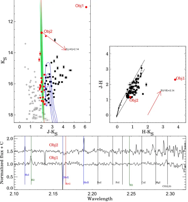
We observed Obj 1 during our SofI 2012 run, together with 2MASSJ12114653-6146070(hereafter Obj 2, Figure4, lower panel). Both objects exhibit emission lines. In Obj 1, the COv

=2–0 first-overtone bandhead appears in weak emission; we also detected strong H2emission as in Caratti o Garatti et al.

(2015), the HeIlines are in absorption, and the Brγline is not detected. Following Bik et al.(2006)thefirst-overtone line CO emission is most probably produced by a circumstellar disk. Obj 2 shows HeI/NIIIand HeIIin emission and weak Brγin absorption, and tacking into account its position on the CMD can be classified as O6-8e. The(J−KS)versusKSdiagram of the region is shown in Figure 4. The statistically decontami-nated most probable cluster members form poorly populated main-sequence(MS)and pre-MS(PMS)branches. The group of stars between(J−KS)of 3.5 and 5 mag andKSbetween 13 Figure 4.Top-left:(J−KS)vs.KSCMD for VVV CL010. Gray circles are comparisonfield stars(selected to have the same as a cluster area), red and dark circles are the most probable MS and PMS+IR-excess cluster members, after statistical decontamination. Stars with spectra are denoted by red circles and are labeled. The best

fit of 2.7 Myr(z=0.020)Geneva isochrone is a solid red line; the green area shows the age interval between 1 and 5 Myr; while the blue solid lines stands for PMS Bell et al.(2014)isochrones for 1.0, 2.0, 4.0, and 8.0 Myr, respectively. The red arrow shows the reddening vector. The top-right panel gives the(J−H)vs.

(H−KS)color–color diagram. The continuous and dashed lines represent the sequence of the zero-reddening stars of luminosity Class I(Koornneef1983)and Class V(Schmidt-Kaler1982), the reddening vectors correspond to the best-fit determination. Bottom: SofI low resolution spectra of Obj 1 and Obj 2.

and 16 mag can be dusty objects along the line of sight or NIR excess sources, which can be expected for the star-forming regions affected by high levels of differential extinction. Unfortunately, only two of the possible IR-excess sources identified from the color–color diagram(G298.2584+00.7406 and G298.2663+00.7354)have GLIMPSE measurements and can be classified as YSO candidates (see Section 5). The spectroscopically calculated values ofE(J−K)=2.24±0.13 and (M−m)0 = 15.4±0.8 (12±4 kpc) of Obj 2 were

adopted as afirst guess for establishing the cluster’s reddening and distance via isochrone fitting, and improved estimates of these parameters were obtained through iterative isochrone

fitting on the(J−KS)versusKSCMD. The MS isochrones for solar metallicity(nearly vertical in this mass range)were taken from the Geneva library (Lejeune & Schaerer 2001) and the PMS isochrones are taken from the Pisa models (Bell et al. 2014). Starting with the spectroscopic reddening and distance estimates, isochrones were shifted along the reddening

vector from their intrinsic positions until the best agreement with the observations was achieved. The stars with KS-band excesses and with large uncertainties are removed before doing thefit. The iterations were stopped when the parameters did not change. Uncertainties tied to the cluster reddening and distance were calculated by accounting for the errors of the bestfit, with quadratically added photometric errors, and errors of isochrone degeneracy in theKS-band for very young clusters. The green area plotted in Figure 4 (left) shows the isochrone intervals from 1 to 5 Myr, which are practically identical. For VVV CL010, a reddening and distance modulus of E (J−K) = 2.14±0.24 and (M−m)0 = 14.55±1.3

(8.13±4.8 kpc)and age of 2.7±1.5 Myr were then adopted. This distance is very different from the kinematic distance of 3.8–5.8kpc obtained for Obj 1 (G298.2620+00.7394) from radial velocity measurements of CO lines (Wu et al. 2004). Following Messineo et al.(2014)we determined the red clump (RC)position in the 10×10 arcmin field around the cluster Figure 5.Top:(J−KS)vs.KSCMD and(J−H)vs.(H−KS)color–color diagram for VVV CL012. The symbols are the same as in Figure4. The red solid line shows the bestfit of the 12 Myr Geneva isochrone. Bottom: OSIRIS low resolution spectra of Obj 1.

center and calculated an RC reddening and distance modulus of 1.4 mag and 13.7(5.56 kpc), respectively, which is close to the kinematic distance of Obj 1. Two explanations of this discrepancy are possible: since our distance was calculated using only one spectroscopic parallax, a nearly vertical MS isochrone, and a poorly populated PMS branch, this leads to large uncertainty; another possibility is that Obj 1 is not a cluster member. More spectroscopic observations are necessary to clarify this point.

3.2. VVV CL012

VVV CL012 was selected from the Borissova et al.(2011) list, where it was described as a small, embedded group containing IR source IRAS 12175-6236. The CMD shows stars following MS and PMS stars, and a few stars with IR-excess (Figure5), four of them are measured by GLIMPSE and satisfy the criteria of Class I/II objects. (see Section 5). The OSIRIS instrument was used to obtain a spectrum of Obj 1. As can be seen in Figure5, no HeIIline is identified in the low resolution

spectra. The Paβ and Brγ lines, as well as HeI, are in absorption, which indicates a spectral class not earlier than B2. In the H-band of the spectrum, the Brackett series hydrogen lines (HI (4–13), (4–12), (4–11), and (4–10)) show weak emission, which can be formed in the surrounding circumstellar material. The EW of the Paβand Brγlines are consistent with the B1-2 V spectral type. The combination of spectroscopic parallax values(E(J−K)=2.1 and(M−m)0=13.55)with

the MS + PMS isochrone fitting yields a reddening and distance modulus for the cluster ofE(J−K)=2.0±0.3 and (M−m)0=14.1±0.7 (6.6±2.1 kpc)and an age between

10 and 12 Myr. The RC distance for thisfield is calculated to be (M−m)0 = 13.96±0.9 (6.2±2.7 kpc), which in this

case is in good agreement with the spectro-photometric distance estimate of VVV CL012.

3.3. VVV CL013

VVV CL013 was selected from the Borissova et al.(2011) list, where it is described as a small, embedded cluster, which Figure 6.(J−KS)vs.KSCMD and and(J−H)vs.(H−KS)color–color diagram for VVV CL013. The symbols are the same as in Figure4, the best-fit isochrone is 3 Myr. Bottom: SOAR and SofI low resolution spectra of Objs 1, 2, and 3.

contains the YSO candidate [MHL2007] G300.3412-00.2190 (hereafter Obj 1; Mottram et al. 2007). The CMD shows a relatively well populated MS and some PMS and IR-excess stars(Figure6). The OSIRIS and SofI instruments were used to obtain spectra of Objs 1, 2 and 3. The spectrum of Obj 1, shown in Figure6, was classified by Mottram et al.(2007)as a YSO candidate on the basis of 10.4 μm imaging MIR observations. G300.3412-00.2190 is bright, with KS = 8.68±0.03 mag and very red with (J − KS) = 4.61 mag. Our spectrum shows numerous hydrogen lines in emission of which Paβ and Brγ(2.17 μm)are the most prominent. Some HeI lines can be identified in absorption. These atmospheric spectral features suggest for the central star a spectral type O8-B0 V. Obj 2 shows only Brγ in emission, no other lines are identified in this region, and the object can be classified as a Be star. Obj 3 shows Brγ and HeI in absorption and is most probably a B2-3 V star. Following the procedures described earlier, we calculate the reddening and distance modulus to the

cluster asE(J−K)=2.1±0.3 and(m−M)0=13.2±1.1

(4.4 ± 2.2 kpc), respectively. The RC distance was not calculated because of very few RC stars in thefield. The best-fit isochrone gives an age of 2–4 Myr. Additionally, we found in the literature a candidate YSO 2MASS J12201528-6253269 (hereafter Obj 4; Robitaille et al. 2008). Fifteen stars were selected from our color–color diagram as stars with a possible IR-excess. Nine of them have GLIMPSE measurements and satisfy the criterion for Class I/II objects(Section5).

3.4. VVV CL059

VVV CL059 was selected from the Borissova et al.(2011) list, where the high reddening of AV≈20 mag and age between 20 and 30 Myr were determined using only photometry and isochronefitting. Later, Morales et al.(2013) pointed out that the cluster must be much younger than 20 Myr and determined a distance of 5.05 kpc, based on a comparison Figure 7.(J−KS)vs.KSCMD,(J−H)vs.(H−KS)color–color diagram, and ISAAC, VLT medium resolution spectra for VVV CL059. The symbols are the same as in Figure4. The bestfits are for 20 Myr(blue)and 316 Myr(red).

with ATLASGAL images. During our ISAAC 2011 run we observed four stars—Objs 1, 3, 4, and 5—selected from the CMD as possible cluster members. Objs 1, 3, and 5 show well defined metal lines of CaI(2.26μm), MgI(2.28μm), and CO-bands, which are similar to late-K/early-M giant spectral types and, thus, these stars are classified as M0 III, K3-5 III, and K0-2 III, respectively (Figure7). However, we cannot exclude a luminosity Class I classification outright for Objs 1 and 3, which is supported by the Messineo et al. (2014)Q1 and Q2 indices. For Obj 4, on the other hand, Brγshows emission, no HI and HeII lines are detected, and a CaI (2.26 μm) triplet shows weak emission. Given the lack of helium lines, this Obj 4 may be a B-star in formation. The statistically decontami-nated CMD contains 73 possible cluster members and shows two evolved giant/supergiant stars (Obj 1 and 3), a well defined MS, and a couple of stars with IR-excess. Thirteen sources with IR-excess are identified and 12 of them are identified as YSO candidates(see Section5). Obj 5 is probably

afield star based on its position on the CMD. Additionally, one high amplitude IR variable from the Contreras Pena(2015)list is found in the field of VVV CL059. We calculated the reddening and distance modulus for the cluster as E(J−K) = 3.0±0.2 and (m–M)0 = 13.3±1.2 mag

(4.6± 2.5 kpc), using red giant branch classification of Obj 1 and 3. The RC distance for the field gives the same value. The best-fit isochrone gives an age of 316±38 Myr. The supergiant classification of these objects puts the cluster much farther at distance of 11.3±2.8 kpc, with an age of 20 Myr. According to Morales et al.(2013)CL059 is classified as still being associated with the parent molecular gas, and thus even the age of 20 Myr might be too old for this stage of evolution, considering that stellar feedback could remove the residual gas in a few Myr. Moreover, Obj 1 has diffuse warm dust/PAH emission in GLIMPSE and is associated with ATLASGAL cold dust emission, which is typical of YSOs. Our low resolution spectra, however, clearly shows the metal lines in Figure 8. (J−KS) vs.KS CMD, (J−H) vs.(H−KS) color–color diagram, and SofI low resolution spectra for Obj 1 (2MASS J12090127-6315597) of [DBS2003]75. The symbols are the same as in Figure4, the best-fit isochrone is 2 Myr.

absorption typical for evolved stars. Unfortunately, there are not sufficient data(e.g., radial velocities, proper motions, high resolution spectra)to verify cluster memberships of the YSOs, to clarify the nature of Objs 1 and 3, and reveal the nature of this unusual cluster.

3.5.[DBS2003]75

The[DBS2003]75 cluster was selected from the Dutra et al. (2003) catalog and is associated with the ESO 95-1 star-forming region and the ultra-compact HIIregion IRAS 12063-6256. The region was first classified as a possible planetary nebulae (Henize 1967), but latter Cohen & Barlow (1980) suggested that it is an HIIregion. Obj1(2MASS J12090127-6315597)was observed during our SofI 2011 run, and shows strong Brγand HI2.06 μm emissions, but weak emission in HeI 2.12 μm. CO could also show weak emission, but it is difficult to say because this feature is at the end of the spectral range(Figure8). Our low resolution spectra do not allow us to

determine the origin of these emission lines. Thus, it is possible that Brγand HI2.06μm arise in the surrounding HIIregion, which is also supported by the relatively flat continuum. As pointed out by Cooper et al. (2013) the HII regions have relatively flat continua, strong HI emission produced in an optically thin ionized region, and often HeIemission. If these emission lines arise from the HIIregion, then the only visible photosphere line from the YSO will be the weak emission in HeI2.12μm, which indicates an early O7-B0 spectral type.

Two stars in thefield are classified as YSO candidates in the literature: 2MASS J12090156-6315429 and [MHL2007] G298.1829-00.7860 (Mottram et al. 2007, hereafter Objs 2 and 3). The statistically decontaminated CMD (Figure 8) contains 71 possible cluster members, nine of which were identified in the Kharchenko et al. (2013) catalog as high probability members. The MS is poorly populated (only 21 members), and few PMS stars and stars with IR-excess are identified. Thus, despite the relatively large cluster radius, most Figure 9.(J−KS)vs.KSCMD,(J−H)vs.(H−KS)color–color diagram, and SofI low resolution spectra for[DBS2003]93. The symbols are the same as in Figure4, blue circles show common stars with the Kharchenko et al.(2013)catalog; the bestfit is 20 Myr.

probably we have a very young, small stellar group, still embedded in dust and gas, rather than an evolved stellar cluster. The kinematic distance to the IRAS 12063-6256 is calculated as 10.5 kpc (Urquhart et al.2013), the RC distance to the field is (m−M)0 = 13.88 (5.9 kpc), while the

spectroscopic distance using the spectral classification of Obj 1 gives 1.94±0.9 kpc. The Kharchenko et al. (2013)

calculated a reddening of 1.05 mag and a distance of 4.6 kpc. The best isochrone fit favors reddening and distance modulus of E(J−K) = 1.5±0.1 and (m−M)0 =

13.5±1.0 (5.0 ± 2.3 kpc), respectively. Thus, we adopted as the distance to the cluster a weighted mean of all measurements, 5.6±3.0 kpc. The stellar group is young, with an age around 2 Myr.

Figure 10.(J−KS)vs.KSCMD,(J−H)vs.(H−KS)color–color diagram and SofI low resolution spectra for[DBS2003]100. The symbols are the same as in Figure4, the blue circles represent stars in common with Kharchenko et al.(2013); the best-fit isochrone is 15 Myr.

3.6.[DBS2003]93

The[DBS2003]93 cluster was selected from the Dutra et al. (2003)catalog and is associated with the RCW 92 star-forming region. The CMD shows a couple of red giant branch stars, MS stars, and some stars with IR-excess(Figure9). Two stars were observed during our SofI 2011 run, named Obj 1 and Obj 2. As can be seen from our low resolution spectra, Obj 1 does not show Brγ; MgIis in weak emission, and CO shows a inverse PCygni profile. The continuum declines toward the red end of the spectrum. Based on this, we conclude that this is a late M-star in formation. In contrast, Obj 2 shows shallow and broad Brγ, the metallic lines are less deep than in Obj 1, and CO also has a PCygni profile. Thus, the star could be a K-dwarf in formation. Both stars are identified in the Kharchenko et al.(2013)catalog and according to their proper motion analysis are cluster members. Of the cluster members identified by our decontamination, ten MS stars and two YSO candidates (DBS93 3 and DBS93 7)are also identified in the Kharchenko et al. (2013) catalog as high probability cluster

members (blue circles in Figure 9). Kharchenko et al. (2013) determined a much larger cluster radius, older age, and smaller reddening. Based on our 2 mag deeper CMD, we determined the visual diameter of the cluster to be 0.72 arcmin. Wefind the reddening and distance modulus of the cluster to be E (J−K) = 2.6±0.3 and (m−M)0=11.62±0.9

(2.1±0.87 kpc), respectively. The best-fit isochrone gives an age of 20±0.5 Myr.

3.7.[DBS2003]100

The [DBS2003]100 cluster was selected from Dutra et al. (2003) and is associated with the RCW 106 star-forming region. The CMD of the cluster is shown in Figure10. It shows a well populated MS and a large number of PMS stars. Some stars with IR-excess can be identified in the color–color diagram(discussed in Section5); two of them, DBS100 ysoc9 and DBS100 ysoc10, are identified in the Kharchenko et al. (2013)catalog with high membership probability. Three stars (Objs 1, 2, and 3)were observed with SofI during the 2011 run. Figure 11.(J−KS)vs.KSCMD,(J−H)vs.(H−KS)color–color diagram, and SofI low resolution spectra for[DBS2003]130. The symbols are the same as in Figure4; the best-fit isochrone is 3 Myr.

All of them show a ratherflat continuum shape, Brγ, HeI, and HeIIin absorption. Objs 1, 2, and 3 are classified as being of O4, O6, and O7 V spectral type, respectively. Despite their very early spectral type all three stars show a CO line in emission, which can be associated with a circumstellar disk or envelope. As in the case of DBS 93 the cluster is part of the Milky Way Star Cluster project(Kharchenko et al.2013), with fundamental parameters as follows: E(J−K) = 0.52; a distance modulus of 2.2 kpc; and an age of 300 Myr. Our spectroscopically calculated reddening and distance modulus give E(J−K) = 1.1±0.1 and (m−M)0 = 12.78±0.8

(3.59±1.3), respectively. The best-fit isochrone confirm the derived spectroscopic distance and reddening and gives an age of 10–15 Myr. As in the case of[DBS2003]93, based on our much deeper CMD, we determine this cluster to be much younger, smaller, and redder than indicated in the Kharchenko catalog.

3.8.[DBS2003]130

The [DBS2003]130 cluster was selected from the Dutra et al. (2003) catalog and is associated with the G305 star-forming region. The CMD of the cluster is shown in Figure11 Figure 12.PDMF of clusters from our sample: from left to right VVV CL010, VVV CL012, VVV CL013, VVV CL059, and[DBS2003]75,[DBS2003]93, and [DBS2003]100. The points show the central position in the mass ranges indicated above them, and the red line corresponds to the Kroupa IMF, while the blue one stands for the bestfit of the data. Bar sizes indicate the mass bin equivalent to each magnitude bin(from the luminosity function)of 1 mag inKS. The lastfigure gives the summary of the slopes.

Table 4. (Continued)

Name GLIMPSE Id. R.A. Decl. J H Ks 3.6 4.5 5.8 8.0

(1) (2) (3) (4) (5) (6) (7) (8) (9) (10) (11)

DBS130 ysoc4 G305.2845-00.0122 198.010098 −62.78972 15.33±0.05 13.63±0.07 11.65±0.03 10.30±0.07 10.09±0.08 9.59±0.07 K K DBS130 ysoc5 G305.2641+00.0009 197.963330 −62.77818 18.33±0.04 16.33±0.01 14.73±0.03 12.69±0.12 11.85±0.26 K K K K

17

The

Astronomical

Journal,

152:74

(

23pp

)

,

2016

September

Borissov

a

e

t

and shows a well populated MS, some PMS stars, and stars with IR-excess(see Section5). Two stars(Objs 1 and 2)were observed with SofI during the 2011 run. As can be seen, Obj 1 shows Brγand HeI(2.06μm)in strong emission, however, the absence of HeIIwould imply an spectral type not earlier than O8. Thus, we assign B0Ie for the spectral type of this star. The spectrum of Obj 2 is similar, but Brγand HeIare less strong, suggesting the B0 Ve spectral type. The combination of spectral parallax and isochrone fit gives a reddening and distance modulus to the cluster ofE(J−K)=2.5±0.2 and (m−M)0=13.1±1.2(4.17±2.3 kpc), which are consistent

with the G305 region distance. The best-fit isochrone gives an age of 3–5 Myr.

4. STELLAR MASS OF THE CLUSTERS

To estimate the total cluster masses, wefirst constructed the cluster present-day mass function(PDMF)using the CMD and then integrated the initial mass function (IMF) fitted to the cluster PDMF. We obtained the cluster PDMF by projecting the MS most probable cluster members, following the reddening vector, to the MS located at the corresponding distance. The MS is defined by the colors and magnitudes given by Cox (2000). The slope Γof the obtained PDMFs of the clusters is given in Table1. As can be seen, theΓvalues are close to the Kroupa IMF (Kroupa2001). After deriving the cluster present-day luminosity function, using 1 KSmag bins, we converted the KSmagnitudes to solar masses using values from Martins et al. (2005) for O-type stars and from Cox (2000) for stars later than O9.5 V. The PDMFs, shown in Figure 12, are fitted and integrated between 0.1Me and the most massive member candidate in each cluster. The

corresponding masses are given in Table 1, where the errors corresponds to thefitting of the IMF to the data, and includes also reddening and distance errors. All clusters in the sample are low or intermediate mass, showing masses between 110 and 1800Me.

5. SEARCH FOR YSO CANDIDATES, VARIABILITY, AND SPECTRAL ENERGY DISTRIBUTION(SED)

To select new YSO candidates in the studied regions we used photometric and variability criteria. First, from the NIR

(J-H) (H-K) color–color diagram of each cluster we selected all stars which are at least 3σ distant from the reddening line that marks the colors of dwarf stars. The list thereby obtained of 90 stars in all clusters was cross-matched with GLIMPSE measurements. Forty-eight of them have photometry from GLIMPSE, and only these objects are proceeded for further inspection. Their coordinates and magnitudes are listed in Table 4 and Figure 13 shows their

[KS−[3.6]], [[3.6]–[4.5]] colors. The objects with

[KS−[3.6]]>0.5 or[[3.6]–[4.5]]>0.5 mag are considered as the most probable Class I and Class II YSOs. These limits are set in order to avoid selecting objects that are more likely Class III objects or normal stars(dashed red line in Figure13). All availableKS magnitude in VSA Data Release 4 (DR4, four year database, up to 30 September 2013,http://horus.roe. ac.uk/vsa/index.html) with grades A and B (e.g., observed within optimal sky conditions) are retrieved to check the variability of the above selected YSO candidates, together with spectroscopically confirmed candidates. The level of variability seen in normal, non-variable stars is estimated to be below 0.1 mag at 12<K_S<16 using apermag3(2″diameter aperture)in the tile catalogs, but we put a 0.2 mag conservative limit marking the errors of the photometry and transformation to the standard system. The saturated stars, the objects with close companions (blending), and those with large photometric errors, ten in total, are removed. To analyze the rest of them we compute a set of variability indexes, namely the StetsonJand K indices(Stetson 1996), the η index (von Newmann 1941), the chi square testχ2(Rebull et al.2015), the small kurtosisκ (Richards et al. 2011), and m

s (e.g., the ratio between the

average KS magnitude from the light curve over the standard deviation of the data). Then we used an unsupervised clustering algorithm, which identify patterns among the values of these indices, separating populations of objects with similar features. Thus, two groups of objects are defined, one with significant amplitudes (in general, greater than 0.2 mag in KS) which shows long and short term variability in the time domain, and another group of sources for which the variability is not very significant, can be confused with noise, and thus is uncertain.

Figures14–16show examples of MJD versusKSmagnitudes for the non-variable and variable stars, respectively. According to our analysis 57% of the YSO candidates show signatures of IR variability. Most of the variable stars in our sample show amplitude variations between 0.2 and 0.5 mag, and only six stars have higher amplitudes. Actually, CL059 Obj2 was taken from the Contreras Pena (2015) list of high amplitude variables, and according to SIMBAD the object CL013 ysoc6 (2MASS J12282798-6257139)is a YSO candi-date; DBS100 ysoc2(2MASS J16202975-5053343)is an AGB candidate; and DBS100 ysoc4 (2MASS J16203226-5052584) is a YSO candidate in the list of intrinsically red stars in the Figure 13. Upper panel: theKS−[3.6],[3.6]−[4.5]color–color plot of 48

variable stars that are detected in GLIMPSE I. The red dashed lines represent the limits used to select Class I and Class II YSOs. The YSO in the clusters are color-coded as follow: VVV CL 010: black; Cl 012: green; CL 013: blue; Cl 059: magenta; DBS 93: pink; DBS 100: red; DBS 130: gray. Lower panel: The(J−H)vs.(H−KS)color–color diagram of the sample. The continuous and dashed lines represent the sequence of the zero-reddening stars of luminosity Class I(Koornneef1983)and Class V(Schmidt-Kaler1982).

Robitaille et al.(2008)paper. We try to determine some periods using different statistic methods, unfortunately, this was not possible on the basis of the existing epochs. Nevertheless, according to the light curves and the position in the CMDs, we consider that the stars CL013 ysoc6, DBS100 ysoc2, DBS100 ysoc4, and DBS130 ysoc5 are most probably semi-regular asymptotic variable stars. It is well known (Robitaille et al.2008)that color-cut photometric selections alone can not distinguish between YSO and AGB stars. However, as we show above, the combination with IR variability analysis can help to solve this problem.

To model the SEDs of the YSO candidates we use the SED models of YSOs developed by Robitaille et al.(2008). We have collected the existing measurements of these objects, from the VVV, 2MASS, GLIMPSE,WISE, and HIGAL catalogs. The respective reddenings and distances of each object are determined by photometry and spectroscopy in Section 3, however due to their large uncertainties, we considered all models that lie within 5σ of the respective errors. The Robitaille models never give a single result, rather, they give a range of models and a chi-squared parameter, an example is shown in Figure17for CL 012 Obj2. The range of models that Figure 14.Examples ofKSmagnitude vs. MJD of non-variable YSO candidates. The solid and dashed red lines mark the 2σand 3σdispersions of the light curve, respectively.

Figure 15.Examples ofKSmagnitude vs. MJD of variable YSO candidates. The symbols are the same as in Figure14.

Figure 16.Examples ofKSmagnitude vs. MJD of variable YSO candidates. The symbols are the same as in Figure14.

give an acceptable chi-squared is usually up to five models starting from the best-fit model in our case, since the HIGAL magnitudes constrains the longer wavelength range. Thus, we calculate the means and standard deviations of the stellar ages, masses, temperatures, and luminosities of the YSOs from the adopted models, which are tabulated in Table 5. Only seven stars are fitted, the rest of the objects do not have enough measurements to construct reliable SEDs. As can be seen from Table5, six of our sources can be classified as massive YSOs, with masses greater that 8 Me, only DBS100 Obj1 is an intermediate-mass objects. All of the objects are very young. The stellar temperatures of the sources range from 4400 to 37000 K. Every SED model shows the presence of an envelope. Only for DBS100 Obj1 the presence of a disk is not detected. It is interesting that Cl010 Obj1 is very massive and has a relatively large amplitude of variability(0.49 mag in KS). Such high variability has rarely been seen in mas-sive YSOs.

6. SUMMARY

In this paper we are reporting some follow-up spectroscopic observations and photometric analysis of eight young stellar clusters projected in the VVV disk area. Using the combination of spectroscopic parallax-based reddening and distance deter-minations with MS and PMS ishochronefitting, we determine the basic parameters (reddening, age, distance)of the sample clusters. The lower mass limit estimations show that all clusters are low or intermediate mass(between 110 and 1800Me), the slope Γof the obtained PDMFs of the clusters is close to the Kroupa IMF. Using VVV and GLIMPSE color–color cuts we have selected a large number of YSO candidates, which are checked for variability, taking advantage of multi-epoch VVV observations. 57% of the YSO candidates are found to show at least low-amplitude variability. In a few cases it was possible to distinguish between YSO and AGB classification on the basis of the light curves. The SEDs of the spectroscopically confirmed YSOs are determined, showing that in general these objects are massive.

We gratefully acknowledge use of data from the ESO Public Survey program ID 179.B-2002 taken with the VISTA telescope, and data products from the Cambridge Astronomical Survey Unit. Support for JB, SRA, RK, MK, MG, GR, MAF, CA-G, DM, CN, NM, PA, JA, and MC is provided by the Ministry of Economy, Development, and Tourism’s Millen-nium Science Initiative through grant IC120009, awarded to The Millennium Institute of Astrophysics, MAS. RK is supported by Fondecyt Reg. No. 1130140, SRA by Fondecyt No. 3140605. MK acknowledges the support by GEMINI-CONICYT project number No. 32130012. MG acknowledges support from Joined Committee ESO and Government of Chile 2014. This publication makes use of data products from the Two Micron All Sky Survey, which is a joint project of the University of Massachusetts and the Infrared Processing and Analysis Center/California Institute of Technology, funded by the National Aeronautics and Space Administration and the National Science Foundation. This publication makes use of data products from the Wide-field Infrared Survey Explorer, which is a joint project of the University of California, Los Angeles, and the Jet Propulsion Laboratory/California Institute of Technology, funded by the National Aeronautics and Space Administration. This work is based in part on observations made with the Spitzer Space Telescope, which is operated by the Jet Propulsion Laboratory, California Institute of Technol-ogy under a contract with NASA.

REFERENCES

Alonso-García, J., Dékány, I., Catelan, M., et al. 2015,AJ,149, 99 Arnaboldi, M., Neeser, M. J., Parker, L. C., et al. 2007, Msngr,127, 28 Baume, G., Carraro, G., & Momany, Y. 2009,MNRAS,398, 221 Bell, C. P. M., Rees, J. M., Naylor, T., et al. 2014,MNRAS,445, 3496 Bik, A., Kaper, L., & Waters, L. B. F. M. 2006,A&A,455, 561 Bonatto, C., & Bica, E. 2010,A&A,516, A81

Borissova, J., Bonatto, C., Kurtev, R., et al. 2011,A&A,532, AA131 Borissova, J., Chené, A.-N., Ramírez Alegría, S., et al. 2014,A&A,569, A24 Caratti o Garatti, A., Stecklum, B., Linz, H., Garcia Lopez, R., & Sanna, A.

2015,A&A,573, AA82

Chené, A.-N., Borissova, J., Bonatto, C., et al. 2013,A&A,549, AA98 Chené, A.-N., Borissova, J., Clarke, J. R. A., et al. 2012,A&A,545, AA54 Figure 17.Four different SEDs models(solid lines)for CL 012 Obj2. The dashed line plots the best-fit photometric model.

Table 5

The Stellar Ages, Masses, Temperatures, and Luminosities of YSOs

Object log(Age) log(Mass) (Me) log(T) (K) log(Disk Mass) (Me) log(Ltot) (Le) log(Env. Mass) (Me)

Note.Note that the errors are also in logarithmic scale.

Chené, A.-N., Ramírez Alegría, S., Borissova, J., et al. 2015,A&A,584, 31C Cohen, M., & Barlow, M. J. 1980,ApJ,238, 585

Contreras Pena, C. 2015, PhD thesis, Univ. Hertfordshire

Cooper, H. D. B., Lumsden, S. L., Oudmaijer, R. D., et al. 2013,MNRAS, 430, 1125

Cox, A. N. 2000, Allen’s Astrophysical Quantities (4th edn.; New York: Springer)

Cross, N. J. G., Collins, R. S., Mann, R. G., et al. 2012,A&A,548, AA119 Crowther, P. A., Hadfield, L. J., Clark, J. S., Negueruela, I., & Vacca, W. D.

2006,MNRAS,372, 1407

Cyganowski, C. J., Whitney, B. A., Holden, E., et al. 2008,AJ,136, 2391 Davies, B., Figer, D. F., Kudritzki, R.-P., et al. 2007,ApJ,671, 781 Dutra, C. M., Bica, E., Soares, J., & Barbuy, B. 2003,A&A,400, 533 Elson, R. A. W., Fall, S. M., & Freeman, K. C. 1987,ApJ,323, 54 Hanson, M. M., Conti, P. S., & Rieke, M. J. 1996,ApJS,107, 281 Hanson, M. M., Kudritzki, R.-P., Kenworthy, M. A., Puls, J., &

Tokunaga, A. T. 2005,ApJS,161, 154 Henize, K. G. 1967,ApJS,14, 125

Henning, T., Schreyer, K., Launhardt, R., & Burkert, A. 2000, A&A,353, 211 Hervé, A., Martins, F., Chené, A.-N., Bouret, J.-C., & Borissova, J. 2016,

NewA,45, 84

Kharchenko, N. V., Piskunov, A. E., Schilbach, E., Röser, S., & Scholz, R.-D. 2013,A&A,558, A53

Koornneef, J. 1983, A&A,128, 84 Kroupa, P. 2001,MNRAS,322, 231

Lejeune, T., & Schaerer, D. 2001,A&A,366, 538

Liermann, A., Hamann, W.-R., & Oskinova, L. M. 2009,A&A,494, 1137 Lumsden, S. L., Hoare, M. G., Urquhart, J. S., et al. 2013,ApJS,208, 11 Martins, F., & Plez, B. 2006,A&A,457, 637

Martins, F., Schaerer, D., & Hillier, D. J. 2005,A&A,436, 1049

Martins, L. P., & Coelho, P. 2007,MNRAS,381, 1329 Mauerhan, J., Van Dyk, S., & Morris, P. 2011,AJ,142, 40

Mauro, F., Moni Bidin, C., Chené, A.-N., et al. 2013, RMxAA,49, 189 Messineo, M., Zhu, Q., Ivanov, V. D., et al. 2014,A&A,571, A43 Meyer, M. R., Edwards, S., Hinkle, K. H., & Strom, S. E. 1998,ApJ,508, 397 Minniti, D., Lucas, P. W., Emerson, J. P., et al. 2010,New A,15, 433 Moisés, A. P., Damineli, A., Figuerêdo, E., et al. 2011,MNRAS,411, 705 Morales, E. F. E., Wyrowski, F., Schuller, F., & Menten, K. M. 2013,A&A,

560, A76

Mottram, J. C., Hoare, M. G., Lumsden, S. L., et al. 2007,A&A,476, 1019 Osterloh, M., Henning, T., & Launhardt, R. 1997,ApJS,110, 71

Ramírez Alegría, S., Borissova, J., Chené, A. N., et al. 2014,A&A,564, LL9 Rayner, J. T., Cushing, M. C., & Vacca, W. D. 2009,ApJS,185, 289 Rebull, L. M., Stauffer, J. R., Cody, A. M., et al. 2015,AJ,150, 175 Richards, J. W., Starr, D. L., Brink, H., et al. 2011,ApJ,744, 192 Robitaille, T. P., Meade, M. R., Babler, B. L., et al. 2008,AJ,136, 2413 Saito, R., Hempel, M., Alonso-García, J., et al. 2010, Msngr,141, 24 Saito, R. K., Hempel, M., Minniti, D., et al. 2012,A&A,537, AA107 Schmidt-Kaler, T. 1982, in Landolt-Borstein, Group VI, Vol. 2 ed.

K. Schaifers & H. H. Voigt(Berlin: Springer), 1

Soto, M., Barbá, R., Gunthardt, G., et al. 2013,A&A,552, AA101 Stetson, P. B. 1996,PASP,108, 851

Straižys, V., & Lazauskaitė, R. 2009, BaltA,18, 19

Urquhart, J. S., Moore, T. J. T., Schuller, F., et al. 2013,MNRAS,431, 1752 von Newmann 1941, The Annals of Mathematical Statistics, 4, 67

Wallace, L., & Hinkle, K. 1997,ApJS,111, 445

Walsh, A. J., Bertoldi, F., Burton, M. G., & Nikola, T. 2001,MNRAS,326, 36 Walsh, A. J., Hyland, A. R., Robinson, G., & Burton, M. G. 1997,MNRAS,

291, 261

Wu, Y., Wei, Y., Zhao, M., et al. 2004,A&A,426, 503