TítuloCoupled thermo hydro chemical mechanical models for the bentonite barrier in a radioactive waste repository

Texto completo

(1)Coupled thermo-hydro-chemicalmechanical models for the bentonite barrier in a radioactive waste repository Author: Alba Mon López. Doctoral Thesis UDC 2017. Advisor: Francisco Javier Samper Calvete. Civil Engineering Ph.D. Program Civil Engineering School.

(2)

(3) Modelos acoplados termo-hidroquímico-mecánicos de la barrera de bentonita de un almacenamiento de residuos radiactivos Autora: Alba Mon López. Tesis Doctoral UDC 2017. Director: Francisco Javier Samper Calvete. Programa de doctorado de Ingeniería Civil E.T.S. Ingenieros de Caminos, Canales y Puertos.

(4)

(5) Dr. Francisco Javier Samper Calvete, Ph.D. from University of Arizona (USA) and the Polytechnical University of Madrid (Spain), Full Professor, certifies that this doctoral thesis, entitled Coupled thermo-hydro-chemical-mechanical models for the bentonite barrier in a radioactive waste repository, has been performed by Alba Mon López under his supervision in order to obtain the Doctor of Philosophy degree with the International Mention by the University of A Coruña. Dr. Francisco Javier Samper Calvete, Doctor por la Universidad de Arizona (EEUU) y por la Universidad Politécnica de Madrid (España), Catedrático de Universidad, certifica que la tesis doctoral con título, Coupled thermo-hydro-chemical-mechanical models for the bentonite barrier in a radioactive waste repository, ha sido desarrollada por Alba Mon López bajo su supervisión para obtener el grado de Doctor y con Mención Internacional por la Universidad de A Coruña.. A Coruña, April 2017 A Coruña, Abril 2017. Alba Mon López. Dr. F. Javier Samper Calvete. PhD. Student. Advisor. Doctorando. Director.

(6)

(7) Acknowledgements I would like to thank Professor Javier Samper for the opportunity to join his research group and performing this dissertation under his supervision. It would have been impossible to complete this dissertation without his inspiration, encouragement, patience and support throughout my graduate research. Most of the research presented in this dissertation has been performed within the framework of the PEBS Project funded by the European Atomic Energy Community's Seventh Framework Programme (FP7/2007-2011) under grant agreement #232598; the CEBAMA Project funded by the European Atomic Energy Community's (Euratom) Horizon 2020 Programme (NFRP-2014/2015) under grant agreement #662147; and the FEBEX-DP Project (Grimsel Phase VI) funded by the FEBEX-DP Consortium. This work has been also supported by ENRESA (Spain), the Spanish Ministry of Economy and Competitiveness (Projects CGL2012-36560 and CGL2016-78281), FEDER funds and the Galician Regional Government (Project 10MDS118028PR and Fund 2012/181 from “Consolidación e estruturación de unidades de investigación competitivas”, Grupos de referencia competitiva). I have also enjoyed a research pre-doctoral contract from the University of A Coruña. I would like to recognize Peter Eriksson from SKB (Sweden) and Georg Kosakowski from PSI (Switzerland) who gave me the opportunity to spend 1 and 3 months, respectively, and brought me the chance to enjoy their research institutions and had very enriching experiences. The stay at SKB was funded by a training scholarship from the LUCOEX project. The research stay at PSI was funded by an INDITEX-UDC scholarship. The models that I performed in my dissertation have relied on measured data from the FEEBX in situ test and the experiments carried out by CIEMAT and UAM. I would like to thank Pedro Luis Martín, Mariví Villar, Ana María Fernández, María Jesús Turrero and Elena Torres from CIEMAT and Jaime Cuevas from UAM for providing these data. I would like to thank also all my colleagues of the research group Agua y Suelo, especially to Luis Montenegro who encouraged and supported me during my research work, Bruno Pisani, Jesús Fernández, Acacia Naves and Yanmei Li. Finally, I would like to dedicate this dissertation to my friends, to my parents and to my husband, Abel, without his confidence and support it would not have been possible to achieve it..

(8)

(9) Agradecimientos Me gustaría agradecer a Javier Samper la oportunidad de trabajar en su grupo de investigación y poder realizar la tesis doctoral bajo su supervisión. Habría sido imposible realizarla sin su inspiración, paciencia y apoyo durante la etapa de realización de la tesis. La mayor parte de este trabajo ha sido desarrollado dentro del marco de proyecto europeo PEBS Project financiado por el “European Atomic Energy Community's Seventh Framework Programme” (FP7/2007-2011) bajo el contrato Nº 232598; el proyecto CEBAMA financiado por “European Atomic Energy Community's (Euratom) Horizon 2020 Programme (NFRP-2014/2015)” bajo el contrato Nº 662147; y el proyecto FEBEX-DP (Grimsel Fase VI) financiado por el Consorcio del Proyecto FEBEX-DP. Este trabajo también ha sido apoyado por ENRESA (España), Ministerio de Economía y Competencia (Proyecto CGL2012-36560 y CGL2016-78281), fondeos FEDER y fondos de la Xunta de Galicia (Proyecto 10MDS118028PR y fondos: 2012/181 de “Consolidación e estructuración de unidades de investigación competitivas”, Grupos de referencia competitiva). También he disfrutado de una un contrato pre-doctoral financiado por la Universidad de A Coruña. Me gustaría agradecerle a Peter Eriksson de SKB (Suecia) y a Georg Kosakowski de PSI (Suiza) la oportunidad de pasar 1 y 3 meses con ellos respectivamente, de participar en sus centros de investigación y llevarme experiencias enriquecedoras. La estancia en SKB fue financiada por una beca del Proyecto LUCOEX, y la estancia en PSI fue financiada por la beca INDITEX-UDC. Los modelos llevados a cabo durante esta tesis han dependido de los datos medidos en el ensayo in situ del proyecto FEBEX y de experimentos de laboratorio de CIEMAT y UAM. Me gustaría agradecerles la aportación de los datos que he necesitado a Pedro Luis Martín, Mariví Villar, Ana María Fernández, María Jesús Turrero, Elena Torres de CIEMAT y a Jaime Cuevas de la UAM. Me gustaría también agradecer la colaboración de mis compañeros del grupo de Agua y Suelo, especialmente a Luis Montenegro quien me ha alentado y apoyado durante el trabajo de investigación, Bruno Pisani, Jesús Fernández, Acacia Naves y Yanmei Li. Finalmente, me gustaría dedicar la tesis a mis amigas, mi padres y a mi marido, Abel, sin su confianza y su apoyo esto no habría sido posible..

(10)

(11) Coupled THCM models of the bentonite barrier in a HLW repository. Coupled thermo-hydro-chemical-mechanical models for the bentonite barrier in a radioactive waste repository. Abstract Compacted bentonite is foreseen in several countries as a backfill and sealing material for high-level radioactive waste (HLW) disposal. The long-term performance assessment and the evaluation of the safety of a HLW repository requires the use of numerical models dealing with the thermal (T), hydrodynamic (H), chemical (C) and mechanical (M) processes and their interplays. This dissertation presents coupled THCM models of the bentonite barrier of HLW repositories in clay and granite. The models account for the geochemical processes taking place within the bentonite as well as the interactions of the bentonite with the concrete liner and the corrosion products of the metallic canister. The THCM code INVERSE-FADES-CORE has been updated, extended to deal with reactive gaseous phases, verified and benchmarked against other codes. Coupled THCM numerical models have been applied to: 1) Small-scale heating and hydration laboratory tests performed by CIEMAT on compacted FEBEX (Full-scale Engineer Barrier Experiment) bentonite and its interactions with corrosion products and concrete; 2) FEBEX mock-up and in situ tests; 3) Long-term reactive transport model predictions of HLW repositories in granite and clay rocks. The results of the numerical models of the lab and in situ tests show a good agreement with the measured data. .. i.

(12)

(13) Coupled THCM models of the bentonite barrier in a HLW repository. Modelos acoplados termo-hidro-químico-mecánicos de la barrera de bentonita de un almacenamiento de residuos radiactivos. Resumen La bentonita compactada es el material previsto para el relleno y sellado de los residuos radioactivos de alta actividad (RAA) en un almacenamiento geológico profundo (AGP). La evaluación del comportamiento y de la seguridad de un AGP requiere utilizar modelos numéricos acoplados térmicos (T), hidrodinámicos (H), químicos (Q) y mecánicos (M). En esta tesis se han desarrollado modelos acoplados THQM de la barrera de bentonita para el AGP en granito y en arcilla. Los modelos tienen en cuenta los procesos geoquímicos que tienen lugar en la bentonita y sus interacciones con el hormigón y con los productos de corrosión del contenedor metálico. Los modelos se han realizado con una versión del código THQM INVERSE-FADES-CORE que se ha mejorado para tener en cuenta el transporte reactivo de gases en la fase gaseosa y se ha verificado y comparado con otros códigos. Se han realizado modelos numéricos THQM de: 1) Ensayos de laboratorio; 2) Ensayos FEBEX (Full-scale Engineer Barrier Experiment) en maqueta e in situ; 3) Predicciones de la evolución geoquímica a largo plazo de la barrera de bentonita en un AGP en granito y en arcilla. Los resultados de los modelos numéricos muestran un buen ajuste a los datos medidos.. iii.

(14)

(15) Coupled THCM models of the bentonite barrier in a HLW repository. Modelos acoplados termo-hidro-químico-mecánicos da barreira de bentonita dun almacenamento de residuos radioactivos. Resumo A bentonita compactada é o material previsto para o recheo e selado dos residuos radioactivos de alta actividade (RAA) nun almacenamento xeolóxico profundo (AXP). A avaliación do comportamento e da seguridade dun AXP precisa de modelos numéricos acoplados térmicos (T), hidrodinámicos (H), químicos (Q) e mecánicos (M). Nesta tese desenroláronse modelos acoplados THQM da barreira de bentonita para o AXP en granito e arxila. Os modelos teñen en conta os procesos xeoquímicos que teñen lugar na bentonita e a súas interaccións co formigón e cos produtos de corrosión do contenedor metálico. Os modelos fixéronse con unha versión do código THQM INVERSE-FADES-CORE que se mellorou para ter en conta o transporte reactivo de gases na fase gaseosa e que se verificou e comparou con outros códigos. Fixéronse modelos numéricos THQM de: 1) Ensaios de laboratorio de hidratación e quecemento de mostras de bentonita FEBEX (Full-scale Engineer Barrier Experiment) compactada e a súas interaccións con produtos de corrosión e formigón; 2) Ensaios FEBEX en maqueta e in situ; 3) Predicións da evolución xeoquímica a longo prazo da barreira de bentonita nun AXP en granito e arxila. Os resultados dos modelos numéricos amosan un bo axuste aos datos medidos.. v.

(16)

(17) Coupled THCM models of the bentonite barrier in a HLW repository. Preface The storage of high-level radioactive waste (HLW) in deep geological repositories (DGR) is based on a multibarrier concept, which includes natural and engineered barriers. The natural barrier is the host rock while the engineered barriers include the waste form, the canister, and the bentonite buffer. Significant research has been performed during the last decades to improve the knowledge, characterize the key parameters and constitutive equations and develop numerical models for the HLW repository barriers. FEBEX (Full-scale Engineered Barrier Experiment) is a demonstration and research project for the engineered bentonite barrier of a HLW repository. FEBEX is based on the Spanish reference concept for radioactive waste disposal in crystalline rock, which consists on the disposal of spent fuel in carbon steel canisters in long horizontal disposal drifts excavated in granite. The main physical, thermal, hydrodynamic, mechanical and geochemical properties of the bentonite were extensively studied during the project. This research has been tackled within the framework of projects funded by the EURATOM Program of the European Commission. Significant parts of this dissertation have been developed within the PEBS (Long-term Performance of Engineered Barrier Systems), CEBAMA (Cement-based materials, properties, evolution, barrier functions) and FEBEX-DP Projects (Full-scale Engineered Barrier Experiment Dismantling Project). The main objective of this dissertation is the updating and the testing of coupled thermal, hydrodynamic, chemical and mechanical (THCM) models for the compacted bentonite barrier in a high-level radioactive waste repository including the following activities: 1) Updating and improving the conceptual and numerical THCM model ; 2) Improving the THCM code INVERSE-FADES-CORE; 3) Modeling laboratory tests; 4) Testing THCM models with data from the FEBEX mock-up and in situ tests; and 5) Evaluation of the long-term geochemical evolution of HLW repositories in granite and clay with reactive transport models.. vii.

(18)

(19) Coupled THCM models of the bentonite barrier in a radioactive waste repository. Contents Coupled thermo-hydro-chemical-mechanical models for the bentonite barrier in a radioactive waste repository .................................................................................................. i Modelos acoplados termo-hidro-químico-mecánicos de la barrera de bentonita de un almacenamiento de residuos radiactivos ........................................................................... iii Modelos acoplados termo-hidro-químico-mecánicos da barreira de bentonita dun almacenamento de residuos radioactivos ........................................................................... v Preface .................................................................................................................................. vii Contents ................................................................................................................................. ix List of Figures.................................................................................................................... xviii List of Tables ................................................................................................................... xxxiii List of terms and abbreviations .................................................................................... xxxvii Chapter 1. Introduction .......................................................................................................... 1 1.1. Motivation and objectives ............................................................................................ 1 1.2. State-of-the-art ............................................................................................................ 2 1.2.1. Bentonite barrier in a radioactive waste repository ...................................................... 2 1.2.2. Bentonite and iron interactions ..................................................................................... 3 1.2.3. Bentonite and concrete interactions ............................................................................. 4 1.2.4. Coupled THCM processes, codes and models ............................................................ 6. 1.3. Scope .......................................................................................................................... 7 Chapter 2. Mathematical formulation of THCM models ...................................................... 9 2.1. Introduction ................................................................................................................. 9 2.2. Coupled THCM processes in a bentonite barrier in a HLW repository ....................... 9 2.3. Mathematical formulation .......................................................................................... 11 2.3.1. Reactive gas transport mathematical formulation ...................................................... 15. Chapter 3. THCM code INVERSE-FADES-CORE ............................................................... 17 3.1. Introduction ............................................................................................................... 17 ix.

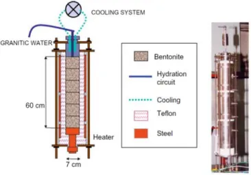
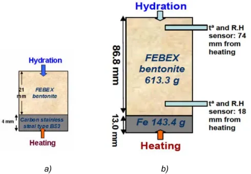
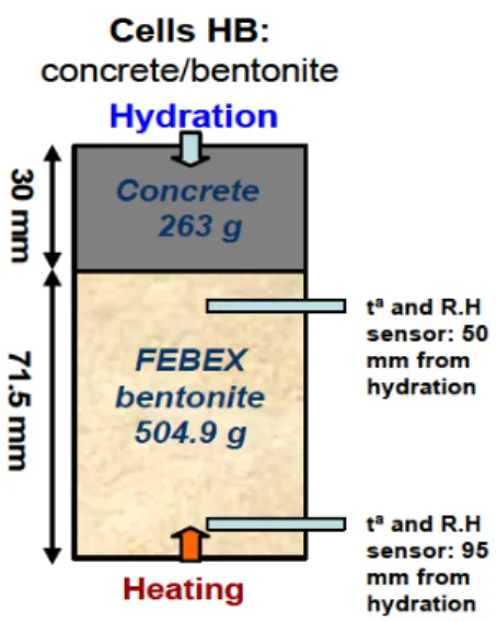
(20) Contents. 3.2. Main features of INVERSE-FADES-CORE ............................................................... 17 3.3. Update of INVERSE-FADES-CORE ......................................................................... 18 3.4. Benchmarking of INVERSE-FADES-CORE V2 ........................................................ 20 Chapter 4. Integrated analysis of thermal, hydrodynamic and chemical data of compacted FEBEX bentonite .............................................................................................. 21 4.1. Introduction ............................................................................................................... 21 4.2. Green-Ampt analytical solutions for water intake ...................................................... 22 4.3. Dimensionless variables ........................................................................................... 23 4.4. Integrated analysis of cumulative water intake data ................................................. 24 4.5. Integrated analysis of water content data ................................................................. 25 4.6. Integrated analysis of temperature data.................................................................... 25 4.7. Integrated analysis of chemical data ......................................................................... 26 4.8. Conclusions............................................................................................................... 26 Chapter 5. Coupled THCM model of the heating and hydration tests on 60 cm long cells ............................................................................................................................................... 29 5.1. Introduction ............................................................................................................... 29 5.2. Test description ......................................................................................................... 29 5.3. Model calibration and results .................................................................................... 31 5.4. Conclusions............................................................................................................... 35 Chapter 6. Coupled THCM models of heating and hydration tests to study the interactions of Fe corrosion products and bentonite ....................................................... 37 6.1. Introduction ............................................................................................................... 37 6.2. Tests description ....................................................................................................... 37 6.3. Model results ............................................................................................................. 38 6.4. Sensitivity analysis .................................................................................................... 41 6.5. Conclusions............................................................................................................... 41 Chapter 7. Coupled THCM model of the heating and hydration concrete-bentonite interactions in the HB4 cell ................................................................................................. 43 7.1. Introduction ............................................................................................................... 43 x.

(21) Coupled THCM models of the bentonite barrier in a radioactive waste repository. 7.2. Test description ......................................................................................................... 43 7.3. Model results ............................................................................................................. 44 7.4. Conclusions............................................................................................................... 46 Chapter 8. Coupled THCM model of the mortar-bentonite interactions in the double interface cells ....................................................................................................................... 49 8.1. Introduction ............................................................................................................... 49 8.2. Test description ......................................................................................................... 49 8.3. Model description ...................................................................................................... 50 8.4. Model results ............................................................................................................. 50 8.5. Sensitivity analysis .................................................................................................... 52 8.6. Conclusions............................................................................................................... 53 Chapter 9. THCM models of the FEBEX mock-up and in situ test ................................... 55 9.1. Introduction ............................................................................................................... 55 9.2. Model testing with data from the FEBEX mock-up test ............................................. 56 9.3. THCM models of the FEBEX in situ test ................................................................... 58 9.3.1. Introduction ................................................................................................................. 58 9.3.2. Testing and updating of the THCM model of the FEBEX in situ test ......................... 59 9.3.3. Pre-dismantling THCM model predictions of the geochemical conditions of the FEBEX in situ test .................................................................................................................................... 62 9.3.4. Predictions of the tracers migration in the FEBEX in situ test.................................... 64 9.3.5. Predictions of the interactions of the bentonite with the concrete plug of the FEBEX in situ test ........................................................................................................................................ 65. 9.4. Conclusions............................................................................................................... 66 Chapter 10. Reactive transport modelling of the long-term interactions of corrosion products and compacted bentonite in a HLW repository in granite ............................... 69 10.1. Introduction ............................................................................................................. 69 10.2. Conceptual and numerical model............................................................................ 69 10.3. Model results ........................................................................................................... 70 10.4. Sensitivity analysis .................................................................................................. 71 10.5. Conclusions............................................................................................................. 72 xi.

(22) Contents. Chapter 11. Long-term non-isothermal reactive transport model of compacted bentonite, concrete and corrosion products in a HLW repository in clay ...................... 73 11.1. Introduction ............................................................................................................. 73 11.2. Conceptual and numerical model............................................................................ 74 11.3. Model results ........................................................................................................... 75 11.4. Sensitivity analysis .................................................................................................. 75 11.5. Conclusions............................................................................................................. 76 Chapter 12. Conclusions and future work ......................................................................... 77 12.1. Improvements in the THCM model and the THCM code ........................................ 77 12.2. Integrated analysis of thermal, hydrodynamic and chemical data of compacted FEBEX bentonite .................................................................................................................... 77 12.3. Coupled THCM models of laboratory test ............................................................... 79 12.4. THCM models the FEBEX mock-up and in situ tests .............................................. 81 12.5. Long-term reactive transport models of the geochemical interactions of the compacted bentonite with concrete and corrosion products in HLW repositories .................. 83 12.5.1. Reactive transport modelling of the long-term interactions of corrosion products and compacted bentonite in a HLW repository in granite .................................................................. 83 12.5.2. Long-term non-isothermal reactive transport model of compacted bentonite, concrete and corrosion products in a HLW repository in clay.................................................................... 83. 12.6. Recommendation for future work ............................................................................ 84 Chapter 13. References ....................................................................................................... 87. APPENDIX. 1.. INVERSE-FADES-CORE. code. improvements,. verification. and. benchmarking ....................................................................................................................... 97 A1.1. Main capabilities of INVERSE-FADES-CORE ........................................................... 98 A1.2. Code improvements ................................................................................................... 99 A1.3. Implementation of the reactive gas transport ........................................................ 100 A1.3.1. Mathematical description of the gas transport equation .................................... 100 A1.3.2. Chemical reactions involving the gaseous and liquid phases ............................ 103 A1.3.3. Code verification ................................................................................................ 104 xii.

(23) Coupled THCM models of the bentonite barrier in a radioactive waste repository. A1.4. Benchmark cases ..................................................................................................... 111 A1.4.1. Non-isothermal geochemical interactions of concrete, bentonite and clay ........ 111 A1.4.2. Atmospheric concrete carbonation .................................................................... 113 A1.5. Description of the changes in the input files ......................................................... 115 A1.6. References ................................................................................................................ 116 APPENDIX 2. Integrated analysis of thermal, hydrodynamic and chemical data of compacted FEBEX bentonite ............................................................................................ 119 A2.1. Introduction ............................................................................................................... 120 A2.2. Heating and hydration experiments on FEBEX bentonite .................................... 122 A2.2.1. FEBEX in situ test .............................................................................................. 122 A2.2.2. FEBEX mock-up test ......................................................................................... 123 A2.2.3. Laboratory experiments ..................................................................................... 123 A2.2.4. Water content data ............................................................................................ 125 A2.2.5. Chemical data .................................................................................................... 126 A2.3. Dimensional analysis ............................................................................................... 127 A2.3.1. Dimensionless variables .................................................................................... 127 A2.3.2. Green-Ampt analytical solutions for water inflow ............................................... 128 A2.4. Results of the dimensional analysis ....................................................................... 131 A2.4.1. Integrated analysis of temperature data ............................................................ 131 A2.4.2. Integrated analysis of cumulative water intake data .......................................... 132 A2.4.3. Integrated analysis of water content data .......................................................... 134 A2.4.4. Integrated analysis of chemical data ................................................................. 137 A2.5. Discussion of results ............................................................................................... 138 A2.6. Conclusions .............................................................................................................. 140 A2.7. References ................................................................................................................ 141 APPENDIX 3. Coupled THCM model of the heating and hydration tests on 60 cm long cells ..................................................................................................................................... 145 A3.1. Introduction ............................................................................................................... 146 A3.2. Test description ........................................................................................................ 146 xiii.

(24) Contents. A3.3. Available data............................................................................................................ 147 A3.4. Model description ..................................................................................................... 150 A3.5. Model calibration ...................................................................................................... 155 A3.6. Model results............................................................................................................. 159 A3.6.1. Thermo-hydro-mechanical results ..................................................................... 159 A3.6.2. Chemical results ................................................................................................ 169 A3.7. Discussion and conclusions ................................................................................... 183 A3.8. References ................................................................................................................ 187 APPENDIX 4. Coupled THCM models of heating and hydration tests to study the interactions of Fe corrosion products and bentonite ..................................................... 189 A4.1. Introduction ............................................................................................................... 190 A4.2. Corrosion tests on small cells................................................................................. 191 A4.2.1. Introduction ........................................................................................................ 191 A4.2.2. Test description ................................................................................................. 191 A4.2.3. Analysis of available data .................................................................................. 192 A4.2.4. Model description............................................................................................... 193 A4.2.5. Model results ..................................................................................................... 199 A4.3. Corrosion tests on medium-size cells .................................................................... 217 A4.3.1. Introduction ........................................................................................................ 217 A4.3.2. Test description ................................................................................................. 217 A4.3.3. Available data .................................................................................................... 219 A4.3.4. Model description............................................................................................... 219 A4.3.5. Model results ..................................................................................................... 220 A4.4. Summary and discussion of results ....................................................................... 229 A4.5. Conclusions .............................................................................................................. 232 A4.6. References ................................................................................................................ 233 APPENDIX 5. Coupled THCM model of the heating and hydration concrete-bentonite interactions in the HB4 cell ............................................................................................... 237 A5.1. Introduction ............................................................................................................... 239 xiv.

(25) Coupled THCM models of the bentonite barrier in a radioactive waste repository. A5.2. Test description and available data ........................................................................ 241 A5.3. Numerical model ....................................................................................................... 243 A5.3.1. Conceptual model .............................................................................................. 243 A5.3.2. Numerical model ................................................................................................ 247 A5.4. Model results............................................................................................................. 250 A5.4.1. Thermo-hydro-mechanical results ..................................................................... 250 A5.4.2. Chemical results ................................................................................................ 252 A5.5. Summary and discussion of results ....................................................................... 262 A5.6. Conclusions and future works ................................................................................ 263 A5.7. References ................................................................................................................ 265 APPENDIX 6. Coupled THCM model of the mortar-bentonite interactions in the double interface cells ..................................................................................................................... 273 A6.1. Introduction ............................................................................................................... 274 A6.2. Test description ........................................................................................................ 274 A6.3. Model description ..................................................................................................... 277 A6.4. Model results............................................................................................................. 284 A6.4.1. Thermo-hydro-mechanical results ..................................................................... 284 A6.4.2. Chemical results ................................................................................................ 285 A6.4.3. Comparison of the results of the double interface test on 2I 3 and 2I 4 cell ...... 298 A6.5. Summary and discussion of results ....................................................................... 300 A6.6. Conclusions .............................................................................................................. 302 A6.7. References ................................................................................................................ 303 APPENDIX 7. Testing and updating of the THCM model of the FEBEX in situ test ..... 307 A7.1. Introduction ............................................................................................................... 308 A7.2. Sensitivity analyses and solute back diffusion analysis ...................................... 310 A7.2.1. Sensitivity analyses ........................................................................................... 311 A7.2.2. Solute back diffusion from the bentonite into the granite ................................... 317 A7.3. 2-D axisymmetric model .......................................................................................... 320 A7.3.1. Model description............................................................................................... 320 xv.

(26) Contents. A7.3.2. Thermal and hydrodynamic results.................................................................... 321 A7.3.3. Cl- concentration results .................................................................................... 338 A7.3.4. Comparison of the results of the 2-D and 1-D axisymmetric models ................. 339 A7.3.5. Sensitivity runs................................................................................................... 343 A7.4. Updated THCM model .............................................................................................. 347 A7.4.1. Improvements and updates of the THCM model ............................................... 347 A7.4.2. Updated model calculations in a hot section ..................................................... 348 A7.4.3. Sensitivity analyses of the updated THCM model ............................................. 352 A7.5. Model testing with measured thermal and hydraulic data collected from 2002 to 2015 ..................................................................................................................................... 355 A7.5.1. Temperatures .................................................................................................... 355 A7.5.2. Relative humidity and water content .................................................................. 359 A7.5.3. Pore water pressures......................................................................................... 363 A7.5.4. Water content and dry density after dismantling ................................................ 364 A7.6. Conclusions .............................................................................................................. 367 A7.7. References ................................................................................................................ 371 APPENDIX 8. Pre-dismantling THCM model predictions of the geochemical conditions of the FEBEX in situ test.................................................................................................... 373 A8.1. Introduction ............................................................................................................... 374 A8.2. Geochemical predictions for the hot section ......................................................... 374 A8.3. Geochemical predictions for the cold section ....................................................... 380 A8.4. Sensitivity of the predictions to the diffusion coefficients ................................... 385 A8.4.2. Hot section ......................................................................................................... 386 A8.4.3. Cold section ....................................................................................................... 386 A8.5. Transport of conservative species from the granite into the bentonite .............. 389 A8.6. Conclusions .............................................................................................................. 390 A8.7. References ................................................................................................................ 392 APPENDIX 9. Predictions of the tracer migration of the FEBEX in situ test................. 393 A9.1. Introduction ............................................................................................................... 394 xvi.

(27) Coupled THCM models of the bentonite barrier in a radioactive waste repository. A9.2. Tracers used in the FEBEX in situ test ................................................................... 394 A9.2.1. Types of tracers ................................................................................................. 394 A9.2.2. Tracer location ................................................................................................... 395 A9.2.3. Tracer sampling plans ....................................................................................... 397 A9.3. Predictions of iodide migration ............................................................................... 401 A9.3.1. Previous iodide migration modelling .................................................................. 401 A9.3.2. Updated iodide migration ................................................................................... 401 A9.3.3. Sensitivity analyses ........................................................................................... 403 A9.4. Predictions of the migration of point tracers ......................................................... 406 A9.4.1. Numerical model ................................................................................................ 406 A9.4.2. Tracer parameters ............................................................................................. 408 A9.4.3. Numerical model results .................................................................................... 408 A9.5. Summary and conclusions ...................................................................................... 414 A9.6. References ................................................................................................................ 416 APENDIX 10. Predictions of the interactions of the bentonite with the concrete plug of the FEBEX in situ test ........................................................................................................ 419 A10.1. Introduction ............................................................................................................. 420 A10.2. Methodology ........................................................................................................... 420 A10.3. Detailed 2-D axisymmetric model ......................................................................... 422 A10.4. 1-D model of the geochemical interactions ......................................................... 425 A10.4.1. 1-D model description ...................................................................................... 425 A10.4.2. 1-D THCM model results ................................................................................. 427 A10.5. Conclusions ............................................................................................................ 439 A10.6. References .............................................................................................................. 441 APPENDIX 11. Reactive transport modelling of the long-term interactions of corrosion products and compacted bentonite in a HLW repository in granite ............................. 443 APPENDIX 12. Long-term non-isothermal reactive transport model of compacted bentonite, concrete and corrosion products in a HLW repository in clay .................... 455 APPENDIX 13. Resumen .................................................................................................... 473 xvii.

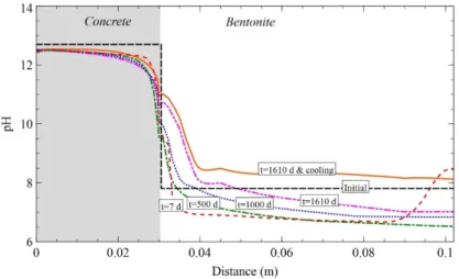
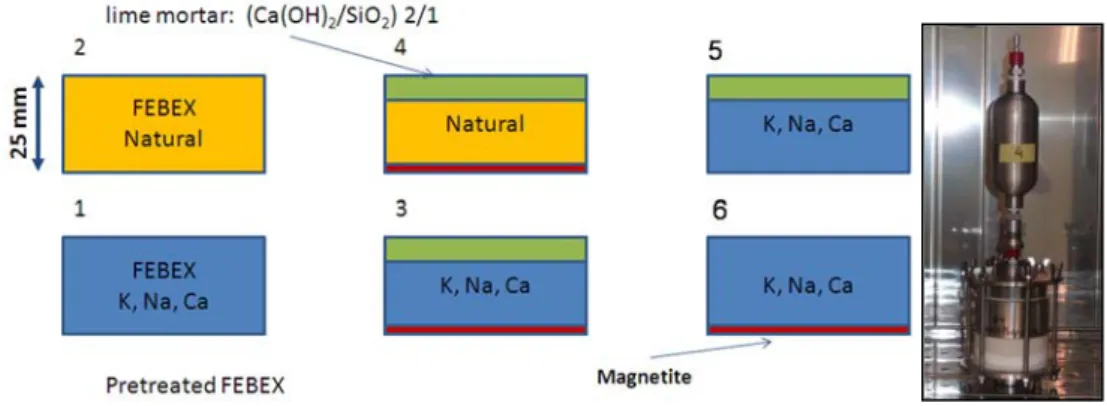
(28) Contents. List of Figures Figure 2.1. Scheme of the couplings between thermal (T), hydrodynamic (H), chemical (C) and mechanical (M) processes..................................................................................................................... 11 Figure 3.1. Computed partial pressure (bar) of CO2(g) at 1 day with INVERSE-FADES-CORE (line) and TOUGHREACT (symbols) for the Case 1. ..................................................................................... 19 Figure 3.2. Calcite volume fractions computed with INVERSE-FADES-CORE (line) and TOUGHREACT (symbols) for the verification Case 4. .......................................................................... 19 Figure 4.1. Schematic design of the in situ test (ENRESA, 2000) (top left), the mock-up test (Martín et al., 2006) (top right), the CT cells (Fernández et al., 1999) (bottom left), and the CG cells (Villar et al., 2008a) (bottom right). ............................................................................................................................ 22 Figure 4.2. Time evolution of the dimensionless cumulative water intake versus dimensionless time for the CT (Fernández et al., 1999) and the CG cells (Fernández and Villar, 2010) and the mock-up test (ENRESA, 2006a)........................................................................................................................... 24 Figure 5.1. Experimental setup of the CG tests (Villar et al., 2008a). .................................................. 30 Figure 5.2. Spatial distribution of the measured (symbols) and computed (line) gravimetric water content at the end of the CG0.5, CG0.5b, CG1, CG1b, CG2, CG2b and CG7.6 tests. ........................ 33 Figure 5.3. Spatial distribution of the measured aqueous extract (symbols) and the computed (lines) Cl- concentrations at the end of the CG0.5, CG0.5b, CG1, CG1b, CG2 and CG2b tests. And comparison of the Cl- concentrations reported by Fernández and Villar (2010) (symbols) and the computed (lines) Cl- concentrations at the end of the CG7.6 test. ........................................................ 33 Figure 6.1. Scheme of the corrosion tests on small cells (left) (Torres et al., 2008) and of the corrosion tests on medium-size cells (right) (Turrero et al., 2011). ....................................................................... 38 Figure 6.2. Spatial distribution of the computed cumulative magnetite precipitation at selected times in the corrosion test on small cell at 100ºC (left) and in the medium-size corrosion test on FB3 cell (right). ............................................................................................................................................................... 40 Figure 6.3. Measured (symbol) and computed (line) weight of precipitated iron hydroxide at the end of in the corrosion test on small cell at 100ºC (t = 180 days) and after cooling. ....................................... 40 Figure 7.1. Scheme of the concrete-bentonite test on HB4 cell (Turrero et al., 2011). ........................ 44 Figure 7.2. Spatial distribution of the computed pH in the HB4 cell at selected times. ........................ 46 Figure 8.1. Scheme of the six double interface tests (Cuevas et al., 2016). ........................................ 50 Figure 8.2. Spatial distribution the computed pH in the double interface 2I3 test at selected times. ... 52 Figure 9.1. Computed (line) and measured (symbols) water intake for the FEBEX mock-up test....... 57 Figure 9.2. Computed (line) and measured (symbols) relative humidity in the sensors located at 0.22 m from the heater for the FEBEX mock-up test. ........................................................................... 57 Figure 9.3. Computed (lines) and measured (symbols) relative humidity in the sensors located at 0.37 m from the heater for the FEBEX mock-up test. ........................................................................... 57 Figure 9.4. Computed (lines) and measured (symbols) relative humidity in the sensors located at 0.55 m from the heater for the FEBEX mock-up test. ........................................................................... 58 Figure 9.5. Computed (lines) and measured (symbols) relative humidity in the sensors located at 0.70 m from the heater for the FEBEX mock-up test. ........................................................................... 58 Figure 9.6. Comparison of the predicted gravimetric water content (lines) in a hot section (left) and a cold section (right) and the measured gravimetric water content data (symbols) in sections S22, S27, S45, S49, S52, S9, S15 and S58 at the times of dismantling of heater 1 (year 2002) and heater 2 (year 2015). The plots at the bottom show the location of the sections where water contents were measured. .............................................................................................................................................. 62 Figure 9.7. Pre-dismantling predictions of Cl- and Ca2+ concentrations (lines) in 2002 and 2015 in a hot section. The graph also shows the inferred Cl- concentrations in sections 19 and 29 in 2002 (symbols). .............................................................................................................................................. 63 Figure 9.8. Pre-dismantling predictions of Cl- and Ca2+concentrations (lines) in 2002 and 2015 in a cold section. The graph also shows the inferred Cl- concentrations in section 12 in 2002 (symbols). . 63. xviii.

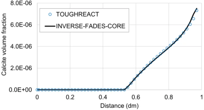
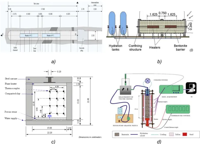
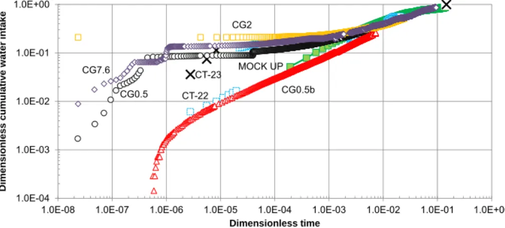
(29) Coupled THCM models of the bentonite barrier in a radioactive waste repository. Figure 9.9. Computed concentrations of dissolved borate (top left), selenate (top right), europium (bottom left) and cesium (bottom right) (mol/L) at 18 years with the 2-D numerical model in a vertical plane normal to the axis of the gallery................................................................................................... 65 Figure 9.10. Predicted pH (left) and changes in porosity caused by dissolution/precipitation reactions (right) in the bentonite and the concrete at selected times. .................................................................. 66 Figure 10.1. Scheme of the engineered barrier system and 1-D finite element grid of the axisymmetric model (Samper et al., 2016). ................................................................................................................. 70 Figure 10.2. Radial distribution of the computed bentonite porosity which changes due to mineral dissolution/precipitation at selected times (Samper et al., 2016). ......................................................... 71 Figure 11.1. 1-D finite element grid which accounts for the canister, the bentonite barrier, the concrete liner and the clay formation (Mon et al., 2017). ..................................................................................... 74 Figure 11.2. Radial distribution of the computed porosity which changes due to mineral dissolution/precipitation at selected times. ............................................................................................ 75. Figure A1.1. 1-D finite element grid used for Case 1 and prescribed partial gas pressures at the boundaries. .......................................................................................................................................... 104 Figure A1.2. Computed partial pressure (bar) of CO2(g) at 1 day with INVERSE-FADES-CORE (line) and TOUGHREACT (symbols). ........................................................................................................... 105 Figure A1.3. Computed time evolution of the partial pressure (bar) of CO2(g) with INVERSE-FADESCORE (line) and TOUGHREACT (symbols) at x = 0.19 dm. .............................................................. 105 Figure A1.4. 1-D finite element grid used for Case 2 and fixed pressure at the left boundary. ......... 106 Figure A1.5. Computed partial pressure (bar) of CO2(g) at t = 0.1 and 1 days with INVERSE-FADESCORE (line) and TOUGHREACT (symbols). ...................................................................................... 106 Figure A1.6. Computed time evolution of the partial pressure (bar) of CO2(g) with INVERSE-FADESCORE (line) and TOUGHREACT (symbols) at x = 0.19 dm. .............................................................. 106 Figure A1.7. 1-D finite element grid used in Case 3 and prescribed pressure profile. ...................... 107 Figure A1.8. Computed calcite volume fraction with INVERSE-FADES-CORE (line) and TOUGHREACT (symbols). .................................................................................................................. 108 Figure A1.9. Computed pH with INVERSE-FADES-CORE (line) and TOUGHREACT (symbols). ... 108 Figure A1.10. Computed Ca2+ concentration with INVERSE-FADES-CORE (line) and TOUGHREACT (symbols). ............................................................................................................................................ 108 Figure A1.11. Computed partial pressure with INVERSE-FADES-CORE (line) and TOUGHREACT (symbols) at t = 0.1 and 1 days. .......................................................................................................... 109 Figure A1.12. Computed calcite volume fraction with INVERSE-FADES-CORE (line) and TOUGHREACT (symbols) at t = 0.1 and 1 days. ................................................................................ 110 Figure A1.13. Computed pH with INVERSE-FADES-CORE (line) and TOUGHREACT (symbols) at t = 0.1 and 1 days. .................................................................................................................................... 110 Figure A1.14. Computed Ca2+ concentration with INVERSE-FADES-CORE (line) and TOUGHREACT (symbols) at t = 0.1 and 1 days. .......................................................................................................... 110 Figure A1.15. Scheme of the near-field geometry and the 1-D axisymmetric conceptual model for the benchmark of the interactions of concrete, bentonite and clay (Berner et al., 2013). ......................... 111 Figure A1.16. Comparison of the mineral volumetric fractions computed with OpenGeos-GEMS and CORE2DV5 at 1 year for the isothermal benchmark case at 25ºC. ..................................................... 112 Figure A1.17. Evolution of liquid saturation during concrete drying computed with TOUGH2 (line), HYTEC (triangles) and INVERSE-FADES-CORE (circles) at selected times..................................... 114 Figure A1.18. Dissolved tracer concentration profiles computed with TOUGHREACT (lines), CRUNCHFLOW (solid squares), MIN3P (crosses), HYTEC (triangles) and INVERSE-FADES-CORE (circles) at selected times. ................................................................................................................... 114 Figure A2.1. Scheme of FEBEX in situ test (ENRESA, 2006a). Vertical lines show the location of the sampling sections (dimensions in meters). ......................................................................................... 121 Figure A2.2. Scheme of the FEBEX mock-up test (Martín et al., 2006). ........................................... 121 Figure A2.3. Scheme of the CG cells (Villar et al., 2008a)................................................................. 124 Figure A2.4. Scheme of the CT cells (Fernández et al., 1999). ......................................................... 124 Figure A2.5. Scheme for parallel flow (left) and radial flow (right). .................................................... 129 Figure A2.6. Comparison of the Green-Ampt analytical solution and the measured cumulative water intake for the mock-up test (Samper et al., 2011b). ............................................................................ 130. xix.

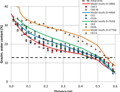
(30) Contents. Figure A2.7. Dimensionless cumulative water intake versus dimensionless time for radial and parallel flow calculated for the same volume and thickness, hydration surface and thickness, volume and hydration surface and calibrated volume, thickness and hydration surface........................................ 131 Figure A2.8. Steady-state dimensionless temperatures versus dimensionless distance for the CT and CG cells and the mock-up and the in situ tests. The error bars show the maximum and minimum temperature fluctuations. ..................................................................................................................... 132 Figure A2.9. Cumulative water intake data for the CT (Fernández et al., 1999) and CG cells (Fernández and Villar, 2010) and the mock-up test (ENRESA, 2006a).............................................. 134 Figure A2.10. Time evolution of the dimensionless cumulative water intake versus dimensionless time for the CT (Fernández et al., 1999) and CG cells (Fernández and Villar, 2010) and the mock-up test (ENRESA, 2006a). .............................................................................................................................. 134 Figure A2.11. Dimensionless gravimetric water content versus dimensionless distance for the CT and CG cells and the mock-up and the in situ tests for dimensionless times ranging from 0.0064 to 0.095. The dimensionless times, tD, are arranged in four figures, a) tD = 0.005, b) tD = 0.01, c) tD = 0.025 and d) tD from 0.071 to 0.095. .................................................................................................................... 136 Figure A2.12. Time evolution of the dimensionless average gravimetric water content for the CT and the CG cells and the mock-up and the in situ tests. ............................................................................ 136 Figure A2.13. Dimensionless Cl- concentration data versus dimensionless distance from the CT and CG cells and the in situ test for selected dimensionless times. .......................................................... 137 Figure A2.14. Minimum, maximum and average pH of the aqueous extracts of the bentonite samples taken from the dismantled of the CT and CG cells and the in situ test versus dimensionless time.... 138 Figure A3.1. Experimental setup of CG tests (Villar et al., 2008a)..................................................... 147 Figure A3.2. Raw data (symbols) and corrected data (discontinuous lines) of cumulative water intake for CG cells. ......................................................................................................................................... 148 Figure A3.3. One dimensional finite element mesh used for the numerical model of the 60 cm long CG cells. .............................................................................................................................................. 151 Figure A3.4. Spatial distribution of the mean measured (symbols) and the computed (lines) temperatures at the end of the CG1 and CG1b tests with the previous and the revised models. ...... 156 Figure A3.5. Spatial distribution of the measured (symbols) and the computed (line) saturation degree at the end of the CG1 and CG1b tests with the previous and the revised models. ............................ 156 Figure A3.6. Spatial distribution of the measured (symbols) and the computed (lines) concentrations of the exchanged Na+, K+, Ca2+ and Mg2+ at the end of the CG0.5b test with the previous and the revised model. ..................................................................................................................................... 158 Figure A3.7. Time evolution of the measured water intake (symbols) for the CG7.6 test and the computed cumulative water intake (lines) for the previous and the revised models. .......................... 159 Figure A3.8. Comparison of the Cl- concentrations of the GMFV reported by Fernández and Villar (2010) (symbols) and the Cl- concentrations at the end of the CG7.6 test computed with the previous and the revised models (lines). ........................................................................................................... 159 Figure A3.9. Spatial distribution of the measured (symbols) and the computed (line) porosity at the end of the CG0.5 and CG0.5b tests. ................................................................................................... 160 Figure A3.10. Spatial distribution of the measured (symbols) and the computed (line) gravimetric water content at the end of the CG0.5 and CG0.5b tests. .................................................................. 160 Figure A3.11. Spatial distribution of the measured (symbols) and the computed (line) saturation degree at the end of the CG0.5 and CG0.5b tests. ............................................................................. 161 Figure A3.12. Time evolution of the measured (symbols) and the computed (line) cumulative water intake of the CG0.5 and CG0.5b tests. ............................................................................................... 161 Figure A3.13. Spatial distribution of the mean measured (symbols) and the computed (lines) temperatures at the end of the CG0.5 and CG0.5b tests.................................................................... 162 Figure A3.14. Time evolution of the measured (discontinuous lines) and the computed (continuous lines) temperatures at the sensors located at x = 0.1, 0.2, 0.3, 0.4 and 0.5 m (from the heaters) of the CG0.5 and CG0.5b tests. .................................................................................................................... 162 Figure A3.15. Spatial distribution of the measured (symbols) and the computed (line) porosity at the end of the CG1 and CG1b tests. ......................................................................................................... 163 Figure A3.16. Spatial distribution of the measured (symbols) and the computed (line) gravimetric water content at the end of the CG1 and CG1b tests. ........................................................................ 163 Figure A3.17. Spatial distribution of the measured (symbols) and the computed (line) saturation degree at the end of the CG1 and CG1b tests. ................................................................................... 164 Figure A3.18. Time evolution of the measured (symbols) cumulative water intake for the CG0.5 test and the computed (lines) water intake of the CG0.5, CG1 and CG1b tests. ...................................... 164. xx.

(31) Coupled THCM models of the bentonite barrier in a radioactive waste repository. Figure A3.19. Spatial distribution of the maximum, the minimum and the mean measured (symbols) and computed (lines) temperatures at the end of the CG1 and CG1b tests. ...................................... 164 Figure A3.20. Time evolution of the measured (discontinuous lines) and the computed (continuous lines) temperatures at the sensors located at x = 0.1, 0.2, 0.3, 0.4 and 0.5 m (from the heaters) of the CG1 and CG1b tests. .......................................................................................................................... 165 Figure A3.21. Spatial distribution of the measured (symbols) and the computed (line) porosity at the end of the CG2 and CG2b tests. ......................................................................................................... 165 Figure A3.22. Spatial distribution of the measured (symbols) and the computed (line) gravimetric water content at the end of the CG2 and CG2b tests. ........................................................................ 166 Figure A3.23. Spatial distribution of the measured (symbols) and the computed (line) saturation degree at the end of the CG2 and CG2b tests. ................................................................................... 166 Figure A3.24. Time evolution of the measured water intake (symbols) for the CG0.5 and CG2 tests and the computed water intake (lines) for the CG0.5, CG1 and CG2 tests. ....................................... 166 Figure A3.25. Spatial distribution of the maximum, the minimum and the mean measured (symbols) and the computed (lines) temperatures at the end of the CG2 and CG2b tests. ................................ 167 Figure A3.26. Time evolution of the measured (discontinuous lines) and the computed (continuous lines) temperatures at the sensors located at x = 0.1, 0.2, 0.3, 0.4 and 0.5 m (from the heaters) of the CG2 and CG2b tests. .......................................................................................................................... 167 Figure A3.27. Spatial distribution of the measured (symbols) and the computed (line) porosity at the end of the CG7.6 test. ......................................................................................................................... 168 Figure A3.28. Spatial distribution of the measured (symbols) and the computed (line) gravimetric water content at the end of the CG7.6 test.......................................................................................... 168 Figure A3.29. Spatial distribution of the measured (symbols) and the computed (line) saturation degree at the end of the CG7.6 test. ................................................................................................... 168 Figure A3.30. Time evolution of the measured water intake (symbols) for the CG0.5, CG2 and CG7.6 tests and the computed cumulative water intake (lines) of the CG0.5, CG1, CG2 and CG7.6 tests. . 169 Figure A3.31. Spatial distribution of the computed temperature at the end of the CG7.6 test. ......... 169 Figure A3.32. Spatial distribution of the measured (symbols) and the computed (lines) Clconcentrations at the end of the CG0.5 and CG0.5b tests. Measured data include aqueous extract and squeezing data (logarithmic scale, top, and natural scale, bottom, for Cl- concentrations). ............... 170 Figure A3.33. Spatial distribution of the measured (symbols) and the computed (line) concentrations of the exchanged Na+, K+, Ca2+ and Mg2+ at the end of the CG0.5b test. ........................................... 171 Figure A3.34. Spatial distribution of the measured (symbols) and the computed (lines) Clconcentrations at the end of the CG1 and CG1b tests. Measured data include aqueous extract and squeezing data (logarithmic scale, top, and natural scale, bottom, for Cl- concentrations). ............... 172 Figure A3.35. Spatial distribution of the measured (symbols) and the computed (line) concentrations of the exchanged Na+, K+, Ca2+ and Mg2+ at the end of the CG1b test. .............................................. 173 Figure A3.36. Spatial distribution of the measured (symbols) and the computed (lines) Clconcentrations at the end of the CG2 and CG2b tests. Measured data include aqueous extract and squeezing data (logarithmic scale, top, and natural scale, bottom, for Cl- concentrations). ............... 174 Figure A3.37. Spatial distribution of the measured (symbols) and the computed (line) concentrations of the exchanged Na+, K+, Ca2+ and Mg2+ at the end of the CG2 and CG2b test. .............................. 175 Figure A3.38. Comparison of the Cl- concentrations of the GMFV reported by Fernández and Villar (2010) (symbols) and the computed (lines) Cl- concentrations at the end of the CG7.6 test (logarithmic scale, top, and natural scale, bottom, for Cl- concentrations). ............................................................ 176 Figure A3.39. Comparison of the Ca2+ concentrations of the GMFV reported by Fernández and Villar (2010) (symbols) and the computed (line) Ca2+ concentrations at the end of the CG7.6 test. .......... 177 Figure A3.40. Comparison of the Mg2+ concentrations of the GMFV reported by Fernández and Villar (2010) (symbols) and the computed (line) Mg2+ concentrations at the end of the CG7.6 test. ........... 177 Figure A3.41. Comparison of the Na+ concentrations of the GMFV reported by Fernández and Villar (2010) (symbols) and the computed (line) Na+ concentrations at the end of the CG7.6 test. ............ 177 Figure A3.42. Comparison of the K+ concentrations of the GMFV reported by Fernández and Villar (2010) (symbols) and the computed (line) K+ concentrations at the end of the CG7.6 test. .............. 178 Figure A3.43. Comparison of the SO42- concentrations of the GMFV reported by Fernández and Villar (2010) (symbols) and the computed (line) SO42- concentrations at the end of the CG7.6 test. ......... 178 Figure A3.44. Comparison of the HCO3- concentrations of the GMFV reported by Fernández and Villar (2010) (symbols) and the computed (line) HCO3- concentrations at the end of the CG7.6 test. ......... 178 Figure A3.45. Spatial distribution of the computed SiO2(aq) concentrations at the end of the CG7.6 test. ...................................................................................................................................................... 179. xxi.

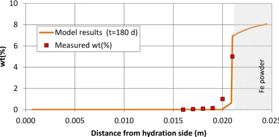
(32) Contents. Figure A3.46. Comparison of the pH of the GMFV reported by Fernández and Villar (2010) (symbols) and the computed (line) pH at the end of the CG7.6 test. ................................................................... 179 Figure A3.47. Spatial distribution of the cumulative dissolution/precipitation of calcite for the CG7.6 test at selected times (positive values for precipitation and negative for dissolution). ........................ 180 Figure A3.48. Spatial distribution of the cumulative dissolution/precipitation of gypsum for the CG7.6 test at selected times (positive values for precipitation and negative for dissolution). ........................ 181 Figure A3.49. Spatial distribution of the cumulative dissolution/precipitation of anhydrite for the CG7.6 test at selected times (positive values for precipitation and negative for dissolution). A zoom of the anhydrite precipitation near the heater is shown on the right.............................................................. 181 Figure A3.50. Spatial distribution of the cumulative dissolution/precipitation of chalcedony for the CG7.6 test at selected times (positive values for precipitation and negative for dissolution). ............ 182 Figure A3.51. Spatial distribution of the measured (symbols) and the computed (line) concentrations of the exchanged Na+, K+, Ca2+ and Mg2+ at the end of the CG7.6 test.............................................. 182 Figure A3.52. Spatial distribution of the concentrations of the sorbed species on the strong, weak #1 and weak #2 sites at the end of the CG7.6 test. ................................................................................. 183 Figure A4.1. Sketch of the corrosion tests on small cells (Torres et al., 2008). ................................. 192 Figure A4.2. Finite element mesh and boundary conditions of the numerical model of the corrosion tests in small cells................................................................................................................................ 194 Figure A4.3. Spatial distribution of the computed (lines) and the measured (symbol) volumetric water content at selected times in the corrosion test on small cell a3 at 100ºC. .......................................... 199 Figure A4.4. Spatial distribution of the computed (lines) and the measured (symbol) saturation degree at selected times in the corrosion test on small cell a3 at 100ºC. ....................................................... 200 Figure A4.5. Spatial distribution of the computed (lines) and the measured (symbol) porosity at selected times in the corrosion test on small cell a3 at 100ºC. ........................................................... 200 Figure A4.6. Spatial distribution of the computed temperature in the corrosion test on small cells at temperatures 25ºC, 50ºC and 100ºC. ................................................................................................. 200 Figure A4.7. Spatial distribution of the computed concentration of dissolved Cl- at selected times in the corrosion test on small cell a3 at 100ºC. ....................................................................................... 201 Figure A4.8. Spatial distribution of the computed concentration of dissolved Na+, K+, Ca2+, Mg2+, HCO3-, SO42- and SiO2(aq) at selected times in the corrosion test on small cell a3 at 100ºC. ........... 203 Figure A4.9. Spatial distribution of the computed concentration of dissolved Fe2+ for 0 < t < 30 days in the corrosion test on small cell a3 at 100ºC. ....................................................................................... 204 Figure A4.10. Spatial distribution of the computed concentration of dissolved Fe2+ for 60 < t < 180 days in the corrosion test on small cell a3 at 100ºC between 60 and 180 days. ................................ 204 Figure A4.11. Spatial distribution of the computed cumulative iron corrosion at selected times in the corrosion test on small cell a3 at 100ºC. (Negative for dissolution and positive for precipitation). ..... 204 Figure A4.12. Spatial distribution of the computed cumulative precipitation/dissolution of magnetite at selected times in the corrosion test on small cell a3 at 100ºC. (Negative for dissolution and positive for precipitation). ....................................................................................................................................... 205 Figure A4.13. Spatial distribution of the computed cumulative precipitation/dissolution of Fe(OH)2(s) at selected times in the corrosion test on small cell a3 at 100ºC. (Negative for dissolution and positive for precipitation). ....................................................................................................................................... 205 Figure A4.14. Measured (symbol) and computed (line) weight of precipitated iron hydroxide at the end of in the corrosion test on small cell a3 at 100ºC (t = 180 days) and after cooling. ............................ 205 Figure A4.15. Spatial distribution of the computed cumulative precipitation/dissolution of goethite at selected times in the corrosion test on small cell a3 at 100ºC. (Negative for dissolution and positive for precipitation). ....................................................................................................................................... 206 Figure A4.16. Spatial distribution the computed cumulative precipitation/dissolution of calcite at selected times in the corrosion test on small cell a3 at 100ºC. (Negative for dissolution and positive for precipitation). ....................................................................................................................................... 206 Figure A4.17. Spatial distribution the computed cumulative precipitation/dissolution of gypsum at selected times in the corrosion test on small cell a3 at 100ºC. (Negative for dissolution and positive for precipitation). ....................................................................................................................................... 206 Figure A4.18. Spatial distribution the computed cumulative precipitation/dissolution of anhydrite at selected times in the corrosion test on small cell a3 at 100ºC. (Negative for dissolution and positive for precipitation). ....................................................................................................................................... 207 Figure A4.19. Spatial distribution the computed cumulative precipitation/dissolution of quartz at selected times in the corrosion test on small cell a3 at 100ºC. (Negative for dissolution and positive for precipitation). ....................................................................................................................................... 207. xxii.