A comparison of wage dynamics in two Latin American countries: different policies, different outcomes

A Comparison of Wage Dynamics in Two Latin American

Countries: Different Policies, Different Outcomes

Luis Carlos Carvajal Osorio∗

This article explores the variations in the wage distribution in two Latin American countries, Bolivia and Colombia, which have had different economic policies in recent years. Using data from household surveys, a decomposition of the wage distribution in each country using Functional Principal Component Analysis is conducted. The results suggest that Bolivia, which has taken left-wing economic policies, has experienced a general increase in wages, especially benefiting the least skilled workers and the

informal sector. On the other hand, the wage distribution in

Colombia, whose economic policy has been focused on free-market principles, has become more concentrated around the median wage, mainly due to changes in the formal sector wages.

JEL: J31; J38; C14

Keywords: Wage dynamics, Functional Principal Component

Analysis, Wage distributions, Wage inequality

Wages are an indicator of the state of the economy and the well-being of the workforce. As economies develop, the structure of the labor market also changes, thereby affecting the wage distribution structure. This paper aims to explore what are the differences in the evolution of the wage distribution in different po-litical contexts by comparing two developing Latin American countries, Bolivia and Colombia, that have taken different political paths. Since 2006, when Evo Morales became president of Bolivia, the country has shifted toward left-wing policies such as an expansion of the public sector and increased levels of social assistance (Canavire-Bacarreza and Rios-Avila, 2015). In contrast, during the same time frame, Colombia has taken policies directed to foster economic growth through free-market principles and the improvement of national security

(Aris-tiz´abal-Ram´ırez et al., 2015).

In spite of the differences in economic policies, Bolivia and Colombia have many similarities. Both countries had a period of fast economic growth in the

∗ _{Escuela de Econom´ıa y Finanzas, Universidad EAFIT, Medell´ın, Colombia.}

late 2000s and early 2010s, mainly driven by the commodites boom of that period. However, both economies are still among the most unequal in the world (World Bank, 2017) and although there have been reductions in the poverty rate in both countries, more than 25% of the population of both Bolivia and Colombia live in poverty (ECLAC, 2016). In addition, the average educational attainment for the population aged 25 or older in Bolivia is 7.8 years, whereas in Colombia it is 8.4 years. In both cases, the educational attainment is below the mean for advanced economies (11 years) (Barro and Lee, 2013). Furthermore, about half of the labor force works in the informal sector (INE, 2017; DANE, 2017). Behrman (1999) notes that low education levels of the workforce and high prevalence of informality are characteristic of labor markets in developing countries. These similarities imply that the effects of the policies on the evolution of wages are more evident, since other possible causes of wage variation like economic growth or labor market composition do not differ by much.

To analyze the evolution of the wage distribution in both countries, I em-ploy a decomposition technique using Functional Principal Component Analysis (FPCA). This method, first developed by Kneip and Utikal (2001) and further extended by Huynh et al. (2011), allows to decompose a family of probability den-sity functions into its mean and a time-specific deviation from the mean. From the FPCA decomposition I obtain a profile of the changes of the wage distribution over time in each country. This allows to compare the dynamics of the distribu-tions and identify the key differences between them. Previous applicadistribu-tions of FPCA decomposition in the context of firm size distribution in the United

King-dom, Canada and Ukraine are found in Huynh and Jacho-Ch´avez (2010), Huynh

et al. (2015) and Huynh et al. (2016) respectively. Chu et al. (2016) use this method to analyze the dynamics of consumer price distributions in the United Kingdom.

This decomposition has a series of interesting characteristics. Since it is a

non-parametric method, there is no a priori restriction about the shape of the

probability density function. Besides, it describes the whole wage distribution, instead of focusing only on the mean wage or certain quantiles. The extension of FPCA proposed by Huynh et al. (2011) to include discrete covariates allows to capture the differences in evolution over time between subsets of the sample, thus providing more information about the changes observed in unconditional probability densities.

The contribution of this article to the literature of wage dynamics is twofold. To the best of my knowledge, this is the first paper to use FPCA decomposition to study the dynamics of wage distributions, thus presenting a novel methodology to study changes in wage distributions over time. Furthermore, I analyze the labor markets in two Latin American economies. By doing so, this article adds to the existing literature on wage distribution and wage dynamics in the region and in developing countries in general (e.g. Atal et al., 2009; Carrillo et al., 2014;

Fern´andez and Messina, 2017).

After applying this technique to data obtained from household surveys in both countries, I found that Bolivia achieved a rather uniform increase in wages during Evo Morales’ presidency, especially benefiting workers with less education and those in the informal sector. On the other hand, between 2008 and 2015 in Colombia, the wage distribution became more concentrated around the median wage. Such change was mostly attributed to changes in the formal sector of the economy. In relation to Bolivia, wage variation in Colombia was distributed more evenly between males and females and between the least and the most educated workers.

This paper is organized as follows: Section II presents some existing litera-ture on wage dynamics and wage determination, while Section III provides some background about labor markets in Bolivia and Colombia. The data are pre-sented along with descriptive statistics for both countries in Section IV. Section V describes the Functional Principal Component Analysis method and its imple-mentation to wage distributions. Results are presented and discussed in Section VI, and Section VII concludes.

II. Review of wage dynamics literature

The literature on wage determinants and wage inequality is very large and the topic has been approached in many different ways. It is generally accepted that individual characteristics like levels of education or work experience imply different wages as they affect labor productivity. However, this is not the only reason behind wage inequality. Labor markets are not perfectly competitive, leading to market failures like considerable market power for certain firms and workers. In addition to these failures, discrimination based on seemingly irrelevant factors such as race or gender also plays an important role in creating wage gaps. Labor market institutions like unions and minimum wages add yet another source of inequality (Blau and Kahn, 1996; Fortin and Lemieux, 1997). This variety of causes explains the interest towards this phenomenon and the wide array of focuses and methods used.

into inequality between the 90th and 50th percentile and inequality between the 50th and 10th percentile. While the 90/50 gap increased during the whole period, the 50/10 gap stabilized after 1987, thus increasing overall inequality, or as the authors describe it, polarizing the labor market even further between skilled and unskilled workers, who have become more prone to be replaced by computers or other machines, further reducing relative demand for unskilled labor.

While SBTC constitutes an important part of the explanation behind wage inequality, the institutional factor cannot be overlooked. Minimum wages, union-ization, labor market regulations and other institutions play an important role in wage determination and equality. For instance, Blau and Kahn (1996) observe that male wage inequality in the United States is higher than in other devel-oped countries, especially at the bottom of the wage distribution. They find that individual characteristics do not fully explain this difference: the low degree of unionization in the United States also contributes towards it as it means that col-lective wage bargaining, which positively affects wages for the least paid workers, is not as common as it is elsewhere. The decline of unionization in the United States in the 1980s had an important effect on wage inequality for males, while the wage gap for females was more affected by the minimum wage (Fortin and Lemieux, 1997). Even and Macpherson (2003) study the effects that minimum wages have on the wage distribution, finding that its effects depend on the pro-portion of the population that earns it and the type of job that pays a minimum wage: if it is an entry-level job, the effect will be on the short run, but it will be more persistent if workers stay in the same job for longer.

This does not mean that technical change and institutions are mutually exclu-sive causes of wage inequality. Weiss and Garloff (2011) reconcile both factors by constructing a model in which technical change affect total productivity, but a transfer mechanism from the most skilled workers to the unskilled workers raises wages for all the workforce. The increase in general wages leads to an excess of supply of unskilled workers creating unemployment, like in the case of continental Europe. The absence of large scale welfare mechanisms means that the differen-tiation of workers by their level of skills is manifested via wage inequality, as it happened in the United States and the United Kingdom in the 1980s and 1990s. Another key component in wage inequality is discrimination based on charac-teristics that have no effect on labor performance. One of the first attempts to measure discrimination were the studies by Blinder (1973) and Oaxaca (1973), who independently developed a method to decompose wage difference into per-sonal attributes and discrimination. Both found high levels of discrimination against women and African Americans. Many authors have explored wage dif-ferences by gender (e.g. Arulampalam et al., 2007; Fang and Sakellariou, 2015; Panizza and Qiang, 2005), usually finding lower wages for women compared to men performing similar jobs. There are two analogous phenomena in female wage distributions: the “glass ceiling,” which is found at the top of the distribution and consists in highly skilled women earning less than comparable men, and the

“sticky floor,” in the bottom of the distribution, consisting in lower wages for the least skilled women in comparison to the least skilled men. Fang and Sakellariou (2015) study wage distribution in the developing world and find that sticky floors are more predominant in Asia and Africa, while glass ceilings are more common in transition economies in Europe (just as discovered by Arulampalam et al., 2007). There is evidence of sticky floors in Latin American countries with low income per capita, like Bolivia and Peru, and glass ceilings in middle income countries, like Uruguay and Brazil (Carrillo et al., 2014).

The difference in wages across sectors has also been the subject of thorough re-search, especially the gap between public and private employers. In general, there is a wage premium for workers in the public sector, and it has been found in both developed countries (e.g. Mueller, 1998 for Canada) and developing economies (e.g. Panizza and Qiang, 2005 and Mizala and Romaguera, 2011, both for Latin America). However, workers at the top of the distribution often have wage penal-ties by working in the public sector (Mueller, 1998; Mizala and Romaguera, 2011). Since the understanding of wage determinants and its dynamics entails many different aspects, the methodological approaches have been just as diverse. Previ-ous studies have used several techniques that consider the wage distribution as a whole in order to examine its evolution over time. For example, Buchinsky (1998) uses quantile regression to estimate wage dynamics for females in the United States. This procedure allows to estimate different rates of return in different points of the wage distribution. DiNardo et al. (1996) develop a semiparametric method to reproduce counterfactual wage distributions by re-weighting distribu-tions based on the population characteristics at the beginning of the period. Melly (2005) combines both methods through a two-step semiparametric approach that allows covariates. First, conditional densities are obtained via quantile regression and then they are integrated to build the unconditional distribution.

Despite the aforementioned differences, labor market in developing countries have been affected by similar shocks to those experienced in developed economies, like SBTC or institutional changes. In India, for example, the returns to higher education increased in the 1990s, particularly benefiting workers who earned the highest wages (Azam, 2012). The author notes that the heterogeneity of returns to education led to an increase in wage inequality in India. An example of the role of institutions in developing labor markets is the study by Bakis and Polat (2015) of the wage changes in Turkey in the 2000s. In that country, wage inequality declined mainly due to a reform in 2004 that increased real minimum wages.

Wage dynamics in Latin America are similar to other developing areas. During the 1980s and 1990s, wage inequality in the region increased, not only because of the technological changes of the time, that had similar effects in developed economies, but also due to some policies implemented during that time frame, like capital market opening, tax reforms or domestic financial sector reforms (Behrman et al., 2000). In recent years, however, the trend has reversed and

some countries have experienced reductions in wage inequality (Fern´andez and

Messina, 2017). These authors found that wage inequality in Argentina, Brazil and Chile declined in the late 1990s and 2000s. They attribute these decreases to changes in the composition of labor markets and to reductions in education and experience premiums. Nevertheless, discrimination is still an important phe-nomenon in Latin America. Atal et al. (2009) analyze the gender and ethnic wage gaps in 18 countries in the region and found that, in average, men are paid 10% more than women and ethnic minorities earn about 13% less than non-minorities. Also, the authors note that there exists great heterogeneity across countries in both gender and ethnic gaps.

III. Background: Labor Markets in Bolivia and Colombia

Bolivia and Colombia have taken different economic policies in the last decade. Under the presidency of Evo Morales, Bolivia’s economic policy has focused on the improvement of the well-being of the population through redistribution and equality, whereas Colombia has taken policies aiming more towards economic

growth and prosperity (Aristiz´abal-Ram´ırez et al., 2015). In spite of the different

approaches in economic policy, both countries have had high rates of economic growth during the last ten years, boosted by the commodities boom during the late 2000s and early 2010s. The average GDP growth rate in Bolivia between 2006 and 2015 was 5.0%, while Colombia’s average GDP growth rate for the same period was 4.6% (World Bank, 2017).

A. Bolivia

Evo Morales was elected in 2005 and in 2006 became the first indigenous and socialist president of Bolivia. During his presidency, Bolivia has distanced itself from the influence of Western institutions and he has passed several economic

reforms like the nationalization of important industrial sectors (e.g. hydrocar-bons, mining), the creation of social welfare programs and the implementation of antidiscrimination law towards indigenous populations. Furthermore, presi-dent Morales increased the royalty taxes for hydrocarbons providing additional revenue used to increase public spending (Hicks et al., 2015; Canavire-Bacarreza and Rios-Avila, 2015).

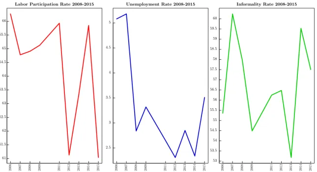
Morales’ presidency has influenced the Bolivian labor market in several ways. Real wages in Bolivia have grown considerably in the last ten years. In 2005, the monthly minimum wage was 440 Bolivianos (US$ 55). By 2015, it had in-creased fourfold, to 1,656 Bolivianos (US$ 238) (Canavire-Bacarreza and Rios-Avila, 2015). In addition, the unemployment rate has been lower than the Latin

American average for the period of study (INE, 2017; ILO, 2017) (see Figure 1).1

However, the job informality rate is over 50% (UDAPE, 2017), and is one of the

highest in the region (ILO, 2017).2

2006 2007 2008 2009 2011 2012 2013 2014 2015

61 61.5 62 62.5 63 63.5 64 64.5 65 65.5 66

Labor Participation Rate 2008-2015

2006 2007 2008 2009 2011 2012 2013 2014 2015

2.5 3 3.5 4 4.5 5

Unemployment Rate 2008-2015

2006 2007 2008 2009 2011 2012 2013 2014 2015

53 53.5 54 54.5 55 55.5 56 56.5 57 57.5 58 58.5 59 59.5 60

Informality Rate 2008-2015

Figure 1. : Labor Market Statistics for Bolivia. Sources: INE (2017); UDAPE (2017)

B. Colombia

The 2000s and 2010s in Colombia have been a period of steady economic growth

and improvement of life conditions. Presidents ´Alvaro Uribe (2002-2010) and

Juan Manuel Santos (since 2010) have managed to significantly reduce the inten-sity of the Colombian armed conflict, thus providing a sense of confidence in the country’s economy. Their economic policies have been targeted to promote

pri-vate investment and free markets (Aristiz´abal-Ram´ırez et al., 2015). Indeed, the

National Development Plan 2010-2014 states that the main goal of the govern-ment is achieving economic prosperity through improvegovern-ments in national security, employment and poverty alleviation (DNP, 2011). Some of the policies that have been carried out in recent years to boost growth and create jobs include the

im-plementation of free trade agreements with Colombia’s main trading partners,3

the privatization of public companies and several reforms to reduce the cost of labor for employers.

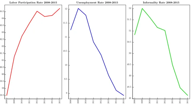
Between 2006 and 2015, the Colombian labor market showed several signs of improvement, in line with the economic situation of this period. Labor partici-pation has had a slight increase, while unemployment and job informality have decreased steadily, although both rates are still above Latin American average (see Figure 2). Real wages in Colombia, however, have not increased much during this time frame. This slow growth in wages has been commonplace in Colombian his-tory, as Urrutia and Ruiz (2010) found after analyzing the behavior of real wages for 170 years. Also, Arango Thomas et al. (2011) discovered that real wages in Colombia are to some extent flexible to changes in labor supply and demand, depending on the economic activity. However, observed rigidities in some sectors and regions may be caused by simultaneous supply and demand shocks. More recently, Morales and Medina (2016) studied the effects on the labor market of a tax reform in 2012 that eliminated 13.5 points of payroll taxes. Such measure was effective in reducing unemployment, but had little effect on wages.

IV. Data

The data used in this paper came from household surveys conducted by the national office of statistics in each country (Bolivia’s Instituto Nacional de tad´ıstica - INE and Colombia’s Departamento Administrativo Nacional de Es-tad´ıstica - DANE). In the case of Bolivia, data encompasses nine years, from

2006, when president Evo Morales took office, to 2015.4 _{On the other hand,}

data from Colombia is available from 2008 to 2015. Household surveys in both countries gather information about sociodemographic characteristics such as gen-der, age, marital status or education, and also contain information regarding the occupation status and the labor conditions of each member of the household.

For this article, I include workers in urban areas in both countries whose ages are between 15 and 65 years old. Following Canavire-Bacarreza and Rios-Avila (2015), I exclude rural workers due to the volatility of rural labor markets. In

3_{Colombia has free trade agreements with the United States, Mexico, the European Union, South} Korea, Chile and the Andean Community of Nations (Bolivia, Ecuador and Peru), among others

4_{Data from 2010 is missing because the INE did not conduct the household survey during that year.}

2008 2009 2010 2011 2012 2013 2014 2015

58.5 59 59.5 60 60.5 61 61.5 62 62.5 63 63.5 64 64.5

Labor Participation Rate 2008-2015

2008 2009 2010 2011 2012 2013 2014 2015

9 9.5 10 10.5 11 11.5 12

Unemployment Rate 2008-2015

2008 2009 2010 2011 2012 2013 2014 2015

48 48.5 49 49.5 50 50.5 51 51.5 52

Informality Rate 2008-2015

Figure 2. : Labor Market Statistics for Colombia. Source: DANE (2017)

total, the dataset contains more than 54,000 observations for Bolivia and over 1.1 million observations for Colombia. In average, there are about 6,000 observations per year for Bolivia, and about 140,000 observations per year for Colombia.

In both Bolivia and Colombia, household surveys inquire about the monthly labor income. To make both measures comparable to each other, I define labor income in the following way: For employed workers, the monthly labor income consists of the net salary, after legal deductions. On the other hand, labor in-come for self-employed workers is the available inin-come for consumption in the household, after discounting the costs related to their occupation.

To account for the differences in income related to differences in hours worked, and to also account for the differences due to full or part time labor, I divide the reported monthly income by the monthly hours worked, thus obtaining hourly wages. Then, I adjust the computed hourly income for inflation using the average annual Consumer Price Index for each country. After obtaining real hourly wages for each country, they are converted to 2010 United States Dollars (USD) using the official exchange rate in each country. Thus, the final wage variable is the logarithm of the real hourly wage, expressed in 2010 USD.

caused by discrepancies in the classification of the workforce.

The education level in this analysis is divided in three levels: the first one, labeled “Primary Education” includes all workers who have no formal education or have only received elementary education. “Secondary Education” gathers those workers that have an education level comparable to high school in the United States (“Secundaria” in Bolivia and “Bachillerato” in Colombia). Finally, the workers who have post-secundary education, either a university degree or technical education, are included in the “Tertiary Education” level. Including education allows to split the workforce by skills, since more education implies higher levels of human capital.

To consider economic sector, I divide the sample into workers in the public and private sectors. A worker belongs to the public sector if he/she works at a public entity of any level (national, regional or local) or if the company where he/she works is owned by the state. Then, I split the private sector into formal

and informal sector using the International Labor Organization definition,5 _that

states that a worker is in the informal sector if he/she is self-employed, a domestic employee, an unpaid employee at family organizations, or works at a firm with five or less employees. If a worker does not fit into any of these criteria, he/she is considered to be working in the formal sector. The distinction of sector is particularly important for developing countries because of the high rates of job informality (see Figures 1 and 2) and because of the differences in rules and institutions between the formal and informal sectors.

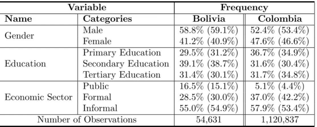
Table 1 shows the composition of the labor market in Bolivia and Colombia respectively. In relation to Colombia, Bolivia has higher participation of males in the workforce and similar levels of education. The rates of informality in both countries are still very high: About half of the workforce in both Bolivia and Colombia work in the informal sector.

Table 1—: Discrete variable categories and relative frequencies. Values in parentheses are corrected for sample weights

Variable Frequency

Name Categories Bolivia Colombia

Gender Male 58.8% (59.1%) 52.4% (53.4%)

Female 41.2% (40.9%) 47.6% (46.6%)

Education

Primary Education 29.5% (31.2%) 36.7% (34.9%)

Secondary Education 39.1% (38.7%) 31.6% (30.4%)

Tertiary Education 31.4% (30.1%) 31.7% (34.8%)

Economic Sector

Public 16.5% (15.1%) 5.1% (4.4%)

Formal 28.5% (30.0%) 37.0% (42.2%)

Informal 55.0% (54.9%) 57.9% (53.4%)

Number of Observations 54,631 1,120,837

5_{See Hussmanns (2004) for a discussion about the definition of informal job and informal sector}

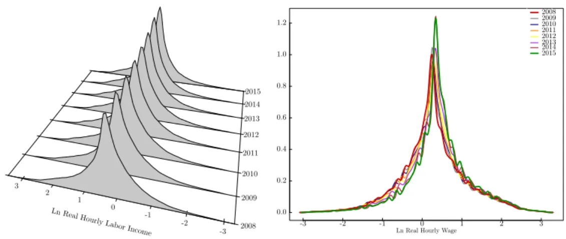
The main descriptive statistics for real hourly wages in each country are in Table 2. Figures 3 and 4 show the wage probability density function by year for Bolivia and Colombia respectively. The graphs on the left of each figure are stacked using the methodology proposed by Hyndman et al. (1996). The graphs on the right show a two-dimensional plot of all the distributions. These figures suggest that real wages in Bolivia have had a steady upward trend during the analyzed period, whereas real wages in Colombia did not increase as much. Instead, the wage distribution in Colombia has compressed around the median, suggesting higher levels of wage concentration. This phenomenon is specially noticed in the last two years of the studied period. In addition, I observe that during the period of study, the mean hourly wage in Colombia was higher than in Bolivia. However, the difference between hourly wages in both countries has narrowed in recent years.

Table 2—: Descriptive Statistics, log Real Hourly Wage in 2010 USD. Numbers in parentheses are corrected for sample weights

(a) Bolivia.

N 54,631

Mean 0.168 (0.120)

Median 0.191 (0.178)

Standard Deviation 0.864 (0.880)

Minimum -5.385

Maximum 5.509

(b) Colombia.

N 1,120,837

Mean 0.344 (0.452)

Median 0.325 (0.315)

Standard Deviation 0.858 (0.862)

Minimum -14.722

Maximum 7.337

It is worth noting that both countries have national minimum wages. However, there are two reasons for which it does not constitute a lower bound for the wage distributions. First, self-employed workers constitute about 40% of the labor force in both countries (INE, 2017; DANE, 2017). Since these workers do not have an employment contract that guarantees the enforcement of minimum wage laws, it is possible for this type of workers to earn less than the minimum wage. Second, the wage distributions used in this article are measured in hours whereas the minimum wage in both countries is expressed in monthly terms for full-time jobs. Legislation in both countries state that no worker can work more than 48 hours a week. Thus, it would be possible to obtain a minimum hourly wage. Nevertheless, data from both countries suggest that this measure is not always enforced. More than 25% of the formal sector workers in the sample in both Bolivia and Colombia work over 48 hours (INE, 2017; DANE, 2017). Therefore, even in companies that comply with minimum wage laws, workers may earn an hourly wage below the equivalent to the minimum hourly wage. Since a lower bound discontinuity point is not present in the data, FPCA can be applied to each family of distributions.

-2 0 2 2006 2007 2008 2009 2011 2012 2013 2014 2015

Ln Real_Hourly

Labor Income -3 -2 -1Ln Real Hourly Wage0 1 2 3

0.0 0.1 0.2 0.3 0.4 0.5

0.6 20062007

2008 2009 2011 2012 2013 2014 2015

Figure 3. : Wage densities by year for Bolivia. Densities were calculated using a second-order Gaussian kernel. The bandwidths were chosen using Silverman’s (1986) rule-of-thumb approximation.

-3 -2 -1 0 1 2 3 2008 2009 2010 2011 2012 2013 2014 2015 Ln Real Hourly

Labor Income -3 -2 -1 Ln Real Hourly Wage0 1 2 3

0.0 0.2 0.4 0.6 0.8 1.0 1.2 2008 2009 2010 2011 2012 2013 2014 2015

Figure 4. : Wage densities by year for Colombia. Densities were calculated using a second-order Gaussian kernel. The bandwidths were chosen using Silverman’s (1986) rule-of-thumb approximation.

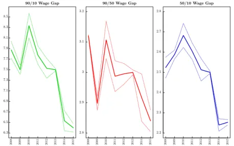
90/10, 90/50 and 50/10 wage gaps across time to examine how has wage inequality changed over time (see Figures 5 and 6). These gaps are calculated by dividing the earnings of the highest percentile by the earnings of the lowest percentile. Measuring these three ratios allows me to assess changes in overall inequality, in the top and in the bottom of the distribution respectively. In both countries wage inequality has decreased significantly. In Bolivia, the main changes in wage inequality are seen in the top of the wage distribution, whereas the reduction in

wage inequality in Colombia is more evident at the lowest wages.

2008 2009 2010 2011 2012 2013 2014 2015 6.8 7 7.2 7.4 7.6 7.8 8 8.2 8.4 8.6 8.8 9 9.2 9.4 9.6 9.8 10 10.2 10.4 10.6 10.8 11 11.2 11.4 11.6 11.8 12 12.2 12.4 12.6

90/10 Wage Gap

2008 2009 2010 2011 2012 2013 2014 2015 2.5 2.6 2.7 2.8 2.9 3 3.1 3.2 3.3 3.4 3.5 3.6 3.7 3.8 3.9 4

90/50 Wage Gap

2008 2009 2010 2011 2012 2013 2014 2015 2.5 2.6 2.7 2.8 2.9 3 3.1 3.2 3.3 3.4

50/10 Wage Gap

Figure 5. : Wage gaps by year - Bolivia. Dotted lines represent the 95% confidence interval

2008 2009 2010 2011 2012 2013 2014 2015 6.3 6.5 6.7 6.9 7.1 7.3 7.5 7.7 7.9 8.1 8.3 8.5

90/10 Wage Gap

2008 2009 2010 2011 2012 2013 2014 2015 2.8

2.9 3 3.1 3.2

90/50 Wage Gap

2008 2009 2010 2011 2012 2013 2014 2015 2.2 2.3 2.4 2.5 2.6 2.7 2.8

50/10 Wage Gap

Figure 6. : Wage gaps by year - Colombia. Dotted lines represent the 95% confidence interval

Table 3—: Mean log Real Hourly Wage (in 2010 USD) by some characteristics - Bolivia

Variable Mean Difference P-Value

Gender Male Female

0.255 0.043 0.212 0.000

Education Tertiary Education Secondary Education or less

0.585 -0.023 0.608 0.000

Sector

Public Formal Private

0.754 0.288 0.466 0.000

Formal Private Informal Private

0.288 -0.070 0.358 0.000

Table 4—: Mean log Real Hourly Wage (in 2010 USD) by some characteristics - Colombia

Variable Mean Difference P-Value

Gender Male Female

0.430 0.250 0.180 0.000

Education Tertiary Education Secondary Education or less

0.913 0.080 0.834 0.000

Sector

Public Formal Private

1.408 0.587 0.820 0.000

Formal Private Informal Private

0.587 0.095 0.492 0.000

V. Functional Principal Component Analysis

A. Overview

Functional Principal Component Analysis (hereafter FPCA) is the adaptation of multivariate Principal Component Analysis (PCA) to functional data. Just as PCA, FPCA is a technique of dimensionality reduction that decomposes data into the most important modes of variation (components). However, as data is functional (each observation is a function defined on a common bounded interval),

components are not random variables defined in Rn, where n is the number of

observations, but random functions defined in the L2 _{space of square-integrable}

functions.

Kneip and Utikal (2001) propose the use of FPCA to characterize the evolution

of a family of probability density functions {ft}Tt=1 over time. Based on the

Karhunen-Lo`eve decomposition, they represent each density of{ft}Tt=1 as follows:

(1) ft=fµ+

L

X

j=1

θtjgj.

Equation (1) states that the FPCA decomposition consists in expressing each

densityft as the sum of the mean of the family of distributions fµ=PTt=1ft/T

and a time-specific deviation from the meanPL_j=1θtjgj. These deviations will be

referred to as deformations, just as in Kneip and Utikal (2001).

In turn, each deformation has two terms: A time-invariant common component

(gj), which corresponds to thej-th eigenfunction from FPCA (Kneip and Utikal,

2001), describing the cross-sectional differences between the distribution in a given year and the common mean distribution, and a time-varying strength coefficient

θtj, that captures the evolution of densities over time, allowing the identification

of the differences and similarities between the distributions (Huynh et al., 2016). The number of components needed to fully characterize the family of probability

density functions is given byL, the number of nonzero eigenvalues of the empirical

covariance operator.

B. Estimation Strategy

As previously described, the FPCA decomposition requires the estimation of the empirical covariance operator. As an alternative, Kneip and Utikal (2001)

propose the following procedure to find gj and θtj. They estimate the T ×T

matrixM, whose elements are defined by

(2) Mts=hft−fµi hfs−fµi ∀t, s,

where the scalar product hξ1, ξ2i is defined byhξ1, ξ2i=

R

ξ1(x)ξ2(x)dx.

The eigenvectors p_r = (pr1, . . . , prT) and corresponding nonzero eigenvalues

λ1 ≥ λ2· · · ≥ λL of the matrix M are related to gj and θtj in equation (1) as follows:

(3) θtr =λ1r/2ptr,

(4) gr=λ−1r /2

T

X

t=1

ptrft=

PT t=1θtrft

PT t=1θ2tr

.

order to account for the heterogeneity of the labor force and assess the differences in wage dynamics across groups.

Let X denote the continuous variable and let Xd _{= {x}d

1, xd2, xd3} be the set

of categorical variables xd

k. The procedure presented by Huynh et al. (2011) to

estimateθtj andgj in (1) has three steps. First, each probability density function

at timetis estimated as follows:

(5) fbt,h =

1

nt

nt

X

i=1

1

hW

x−Xit

h

L_υ,xd_,Xd

it.

In equation (5),W(·) is a univariate kernel estimator for the continuous variable

andL_υ,xd_,Xd

it =

Qr

s=1l(xds, X

ds

it , υ) is the product kernel estimator of the discrete

variables. The bandwidth used in the kernel estimation of the continuous variable

is h, whereas υ is the bandwidth vector used for the kernel estimation of the

discrete variables.

Using these estimations, the elements ofMc, the estimator ofM, are computed

using equation (2).

The eigenvectors p_r = (pr1, . . . , prT) and corresponding nonzero eigenvalues

λ1 ≥λ2· · · ≥λT of the matrix Mc are then calculated. θbtr and bgr are estimated analogously to (3) and (4), but using a different set of kernel estimators with

bandwidthb:

(6) θbtr =λb1r/2pbtr,

(7) _bgr=bλ−1r /2

T

X

t=1 b

ptrfbt,b=

PT t=1θbtrfbt PT

t=1θb2tr

.

Huynh et al. (2011) prove that their method keeps the consistency of θtr and

the asymptotic normality ofgr.

The bandwidth choice strategy is the one adopted by Huynh et al. (2016). First, I use Silverman’s (1986) rule-of-thumb approximation to calculate the bandwidth

for the wage distributions ˜band indicator functions to compute bandwidths for the

discrete variables. These bandwidths are then rate-corrected by settingbh= ˜b5/4

and bb = ˜b×T−1/5 _{respectively, as suggested by Kneip and Utikal (2001) and}

Huynh et al. (2011). To check the robustness of the results to bandwidth selection, I also compute cross-validated maximum likelihood bandwidths and recalculate

the estimations using this new set of bandwidths.6

VI. Results

I present the results from the FPCA decomposition in four parts. First, the dynamic scree plots are shown to select how many components are needed for explaining a good proportion of the total density temporal variability. Second,

I use the dynamic strength components θbtr to analyze the evolution of the wage

distribution over time. Third, the common components_bgr are presented to

iden-tify the points in the distribution where the changes have occurred. Finally, I present total deformations to show the overall movement of the wage distribution and to explore how different groups of the labor force have contributed to total variation.

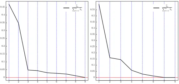
A. Dynamic Scree Plot

The dynamic scree plots (Figure 7) gather the proportion of total change in

the distribution attributable to each component j by plotting the ratio of each

estimated eigenvalueλbj and the total sum of estimated eigenvaluesPTi=1bλi. In

the analysis for Bolivia, the first two components explain an important proportion of total variation (47.2% and 34.5% respectively). For Colombia, the first two components contribute to 59.5% and 16.1% of total variation respectively. In order to explain as much of the variation as possible, the first two components will be used for each country.

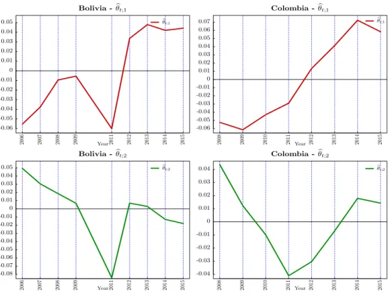
B. Dynamic Score Components

The dynamic score componentsθbtrcapture the evolution over time of the family

of wage distributions. The first two dynamic score components for Bolivia and Colombia are plotted in Figure 8.

The dynamic score components for Bolivia change over time in opposite direc-tions, except for two periods: both of them decrease in 2011 and increase in 2012. The second dynamic score component, while decreasing after 2012, has values closer to zero than first dynamic score component in the same time frame. Then, the net effect is positive and the wage distribution moves toward higher values.

In the case of Colombia,θbt,1 shows an increasing trend across almost the whole

time frame, only starting to decrease after 2014, suggesting a slow but constant

growth in wages. On the other hand,θbt,2 has a downward trend until 2011, when

it begins to recover. The joint movement of both components suggests a sluggish evolution of wages between 2008 and 2013, with moderate growth in 2014 and 2015.

1 2 3 4 5 6 7 8 9 0

0.05 0.1 0.15 0.2 0.25 0.3 0.35 0.4

0.45 _Pbλt

9

t=1bλt

1 2 3 4 5 6 7 8

0 0.05 0.1 0.15 0.2 0.25 0.3 0.35 0.4 0.45 0.5 0.55

bλt

P8

t=1bλt

Figure 7. : Dynamic Scree Plot for Bolivia (left) and Colombia (right)

As dynamic score components measure changes over time for the wage distribu-tion, I contrast them with some macroeconomic series. The correlation coefficients of the first two dynamic score components with select macroeconomic variables are presented in Table 5. These correlations are useful to understand how wages respond to changes in the economic situation of the country.

In Bolivia, the first dynamic score component is correlated negatively with the unemployment and informality rates. Furthermore, the correlation of the first dy-namic strength component with GDP per capita growth is positive, in line with the findings of several authors (e.g. King and Rebelo, 1999; Xu et al., 2015). The correlation with the investment/GDP ratio and the first component is also posi-tive. This points to a raise in wages due to increased labor demand. The second dynamic strength component has negative correlation with occupation rates and GDP per capita growth, while it is positively correlated to unemployment and informality. These signs are consistent with an increase in wages due to reduced labor supply. Nevertheless, considering that the first component explains a higher share of total variation, the demand effect seems stronger.

In Colombia, there is strong positive correlation between the first common com-ponent and occupation rates, coupled with strong negative correlation between wages and unemployment. This points to the transmission of levels of employ-ment to wages. The signs suggest that this change is related to increased labor demand. Contributing to this hypothesis is the high positive correlations between this component and investment/GDP ratio: as investment grows, labor demand increases. This strong relation does not hold with GDP growth. The correlation coefficient is positive but small. Robin (2011) finds that wages in the middle of the distribution are less procyclical than those in the extremes. Since wage

Year

2006 2007 2008 2009 2011 2012 2013 2014 2015 -0.06 -0.05 -0.04 -0.03 -0.02 -0.01 0 0.01 0.02 0.03 0.04

0.05 bθt;1

Bolivia -θbt;1

Year

2006 2007 2008 2009 2011 2012 2013 2014 2015 -0.08 -0.07 -0.06 -0.05 -0.04 -0.03 -0.02 -0.01 0 0.01 0.02 0.03 0.04

0.05 bθt;2

Bolivia -θbt;2

Year

2008 2009 2010 2011 2012 2013 2014 2015 -0.06 -0.05 -0.04 -0.03 -0.02 -0.01 0 0.01 0.02 0.03 0.04 0.05 0.06

0.07 bθt;1

Colombia -bθt;1

Year

2008 2009 2010 2011 2012 2013 2014 2015 -0.04 -0.03 -0.02 -0.01 0 0.01 0.02 0.03

0.04 bθt;2

Colombia -bθt;2

Figure 8. : First two Dynamic Score Componentθbtr evolution: θbt1 (top)θbt2(bottom) for Bolivia (left) and Colombia (right)

tribution in Colombia is very concentrated around the median, total correlation should be smaller than it would be if the distribution had higher standard devi-ation. This might also explain why the correlation of wages and GDP growth is larger in Bolivia. Correlations of the second dynamic strength components with the unemployment and informality rates are negative, as in the case of the first component. Nevertheless, correlations with occupation rate and GDP growth are negative. These facts reinforce the hypothesis that the changes in wages have been due to shifts in labor demand, but also suggest that wages in Colombia are not very sensitive to the economic cycle.

C. Common Components

Common components ˆgr gather the cross-sectional differences between a

distri-bution for a given set of categories and the mean distridistri-bution. From Equation

Table 5—: Correlation coefficient ofθb_t,1andθb_t,2and some macroeconomic variables. Source of

macroe-conomic series: DANE (2017), World Bank (2017), INE (2017)

(a) Bolivia

Variable Correlation with θbt,1 Correlation with θbt,2

Unemployment Rate -0.555 0.585

Occupation Rate -0.477 -0.214

Informality Rate -0.419 0.250

GDP per capita growth 0.389 -0.131

Inflation Rate -0.371 -0.158

Investment/GDP ratio 0.573 -0.758

(b) Colombia

Variable Correlation with θbt,1 Correlation with θbt,2

Unemployment Rate -0.972 -0.051

Occupation Rate 0.871 -0.451

Informality Rate -0.917 -0.297

GDP per capita growth 0.261 -0.615

Inflation Rate -0.319 0.657

Investment/GDP ratio 0.855 0.214

values for the categorical variables.7 _{In this case, there are 2·3·3 = 18 different}

combinations. To summarize the behavior of all the bgr, they are summed and

gathered in theTotal Common Components (TCC) ˜gr:

˜

gr =

X

xd i∈Xd

b

gr.

The first two TCC for Bolivia and Colombia are displayed in Figure 9. In the case of Bolivia, both common components shows the change from low levels of wage toward higher levels, as seen in the evolution of the wage distribution across time (Figure 3). On the other hand, the first common component for Colombia shows little deviation in the extreme values and a large movement around the median of the distribution, consistent with the concentration of wages around the median. The second common component for Colombia shows volatility in the center of the distribution while also presenting little difference in the extremes of the distribution.

7_{Since calculating}

b

grentails the estimation offb_t,b, the bandwidths vector change as the values of the

categorical values change, leading to different kernel estimations and different common components.

-2 -1 0 1 2 Ln Real Hourly Wage

-2 -1 0 1

2 Bolivia _{˜g1 ˜g2}

-2 -1 0 1 2 3

Ln Real Hourly Wage -4

-3 -2 -1 0 1 2 3 4 5

6 ˜g1 ˜g2

Colombia

Figure 9. : Bolivia - First two Total Common Components ˜gr=P_xd

i∈Xdbgr r= 1,2.

D. Dynamic Deformations

The dynamic deformation θbtrbgr shows the overall movement of the density

across time. It combines the differences across time due to different dynamic

score componentsθbtr and the cross-sectional differences captured by the common

components_bgr.

To provide a general view of the changes, I employ TCC (˜gr). Total deformation

in periodtfor component r is equal to:

˜

grθbtr =

X

xd i∈Xd

b

grθbtr.

TCC can be decomposed to reflect the total component for a specific value kof

any discrete variable xd

j. By computing total components for specific values, it

is possible to analyze the wage dynamics for specific subsets of the population. From the total components for a specific category, it is possible to obtain the total deformation for such value:

(8) ˜gr(·, xdj =k)θbtr =

X

xd i, xdj=k

b

Note that the θbtr used in computing the conditional total deformation in (8) are the same as those used in the unconditional total deformation. Hence, the relationship between conditional and unconditional total deformation depends

only on ˜gr. Using this result, Huynh et al. (2016) calculate the share of variation

accounted for by each value of the discrete variable by regressing ˜gr(·, xdj =k) on

˜

gr.

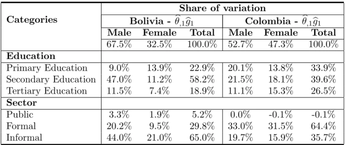
In the remainder of this section, only the first (and largest) component de-formation will be analyzed for brevity. Moreover, even though it is possible to obtain deformations for all periods, this analysis will focus on the deformations on the first and the last periods in order to obtain the combined deformation over the period of interest. The proportion of change according to each value of the discrete variables included in the estimation for the first components in each country are presented in Table 6.

Table 6—: Share of variation accounted for by each category of the discrete variables

Categories

Share of variation

Bolivia - θb,1gb1 Colombia - θb,1gb1

Male Female Total Male Female Total

67.5% 32.5% 100.0% 52.7% 47.3% 100.0%

Education

Primary Education 9.0% 13.9% 22.9% 20.1% 13.8% 33.9%

Secondary Education 47.0% 11.2% 58.2% 21.5% 18.1% 39.6%

Tertiary Education 11.5% 7.4% 18.9% 11.1% 15.3% 26.5%

Sector

Public 3.3% 1.9% 5.2% 0.0% -0.1% -0.1%

Formal 20.2% 9.5% 29.8% 33.0% 31.5% 64.4%

Informal 44.0% 21.0% 65.0% 19.7% 15.9% 35.7%

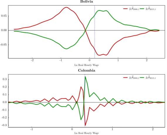
Figure 10 shows the total deformation for the first component (˜g1θbt;1) for both

countries. In Bolivia, the magnitude of the changes in density is not very large, but it occurs at a large interval of values, which means that the raise in wages in Bolivia has been rather uniform. The behavior of the wage deformation is similar in either side of the median, further supporting the idea of an uniform growth in wages. The deformation for 2006 has slightly larger absolute values than the one for 2015, leading to a moderate increase in wage concentration.

In the case of Colombia, total deformation for the first component suggests that both tails of the distribution have stayed stable through time. Changes to the left of the median have been less drastic but encompass a wider interval of values. The largest two peaks of variation are around the median, suggesting an important increase in wage concentration. Moving to the right tail of the distribution, variation is higher than that of the left tail but occurs in a smaller interval, thus fading away faster. Summarizing, the movement of the whole wage distribution in Colombia between 2008 and 2015 can be described as a slight growth in wages, paired to a considerable increase in wage concentration around

the median wage.

Ln Real Hourly Wage

-2 -1 0 1 2

-0.05 0.00 0.05

˜

g1bθ2006,1 g˜1bθ2015,1

Bolivia

Ln Real Hourly Wage

-1 0 1 2

-0.3 -0.2 -0.1 0.0 0.1 0.2

0.3 ˜g1bθ2008,1 g˜1bθ2015,1

Colombia

Figure 10. : Total deformation for the first component - Bolivia (top) and Colombia (bottom). The dotted line represents the median wage, corrected for sample weights

In the following subsections, I analyze how total change is distributed between different groups of the workforce by comparing the total deformation for a specific category to the total deformation of the wage distribution.

Differences by gender. — The differences of wage evolution by gender in

Bolivia and Colombia are depicted in Figure 11 The changes in wages in Bolivia have been mainly due to changes in male wages, who have benefited from both a decrease in the proportion of workers who earn low wages and an increase in the proportion of workers earning higher wages. Female wages have had a similar behavior, but its magnitude has been smaller. Women only have bigger shares of variation at both extremes of the distribution

however that females who earn low salaries had smaller variation in wages than low-paid males. As wages increase, so does the proportion of change attributable to variations in female wages.

Ln Real Hourly Wage

-2 -1 0 1 2

-0.05 0.00 0.05

˜

g1bθ2006,1 g˜1bθ2015,1

Bolivia - Male (67.5%)

Ln Real Hourly Wage

-2 -1 0 1 2

-0.05 0.00 0.05

˜

g1bθ2006,1 g˜1bθ2015,1

Bolivia - Female (32.5%)

Ln Real Hourly Wage

-1 0 1 2

-0.3 -0.2 -0.1 0.0 0.1 0.2

0.3 ˜g1θb2008,1 g˜1θb2015,1

Colombia - Male (52.7%)

Ln Real Hourly Wage

-1 0 1 2

-0.3 -0.2 -0.1 0.0 0.1 0.2

0.3 ˜g1θb2008,1 g˜1θb2015,1

Colombia - Female (47.3%)

Figure 11. : Total deformation by gender: male (top) and female (bottom) in Bolivia (left) and Colombia (right). Percentages show the share of total variation attributed to each group. The darker shaded area represents total deformation in the first year studied (2006 for Bolivia and 2008 for Colombia), and the lighter shaded area represents total deformation in 2015. The dotted line represents the median wage, corrected for sample weights

In Colombia, female wages in the bottom of the distribution did not change as much as the male wages. Given that on average women earn less, this reduced share could point to a sticky floor phenomenon. Such phenomenon is not as evident in Bolivia, where women who earned the lowest wages had more variation than men.

Differences by education. — The education level of the workforce in Bolivia

and Colombia is not very dissimilar, but the shares of wage variation received by each type of workers have noticeable differences. While in both countries, the most educated workers receive the smallest share of the change in wages, Colom-bian workers with tertiary education are accountable for a larger proportion of total change than their Bolivian counterparts, as it can be seen in Figure 12. Indeed, over half of the total variation in wages in Bolivia has been received by

workers with secondary education. Furthermore, workers with secondary educa-tion contribute more to total variaeduca-tion than more educated workers in all levels of remuneration, in contrast to Colombia, where despite their smaller contribution to total wage variation, the most skilled workers explain most of the variation at the highest levels of remuneration. This indicates that in Bolivia, more education does not translate into higher variation in wages.

Another difference between the wage dynamics in both countries is that Colom-bian females with higher education explain a larger proportion of total wage variation than similarly educated males, while in Bolivia males receive higher percentages of the total wage change. This means that the Colombian gender wage gap is reduced as education levels increase. In Bolivia, the opposite is true: female workers with primary education are accountable to higher shares of total wage variation. For Bolivian women, increasing their education level does not imply improving their participation in total wage change.

Ln Real Hourly Wage

-2 -1 0 1 2

-0.05 0.00 0.05

˜

g1bθ2006,1 ˜g1θb2015,1

Bolivia - Primary Education (22.9%)

Ln Real Hourly Wage

-2 -1 0 1 2

-0.05 0.00 0.05

˜

g1bθ2006,1 ˜g1θb2015,1

Bolivia - Secondary Education (58.2%)

Ln Real Hourly Wage

-2 -1 0 1 2

-0.05 0.00 0.05

˜

g1bθ2006,1 ˜g1θb2015,1

Bolivia - Tertiary Education (18.9%)

Ln Real Hourly Wage

-1 0 1 2

-0.3 -0.2 -0.1 0.0 0.1 0.2

0.3 ˜g1bθ2008,1 ˜g1θb2015,1

Colombia - Primary Education (33.9%)

Ln Real Hourly Wage

-1 0 1 2

-0.3 -0.2 -0.1 0.0 0.1 0.2

0.3 ˜g1bθ2008,1 ˜g1θb2015,1

Colombia - Secondary Education (39.6%)

Ln Real Hourly Wage

-1 0 1 2

-0.3 -0.2 -0.1 0.0 0.1 0.2

0.3 ˜g1bθ2008,1 ˜g1θb2015,1

Colombia - Tertiary Education (26.5%)

Differences by sector. —In Figure 13, total wage deformation for both coun-tries is split into economic sector. In the case of Bolivia, two facts stand out: First, even though the Bolivian public sector employ more than 15% of the work-force, it does not have a large contribution to total wage variation. Second, more than half of total wage change in Bolivia is accountable to the informal sector, implying that workers in the formal sector have not benefited as much from the general wage increase as informal workers have. This might be a hindrance to-wards job formalization, since workers can have larger increases in wages if they remain in the informal sector.

The case of Colombia is the opposite of Bolivia, as the formal sector is the main contributor to wage variation. It is worth noting that like Bolivia, Colombia does have high levels of job informality. Another remarkable result from Colombia is that real wages in the public sector have remained stable between 2008 and 2015.

Ln Real Hourly Wage

-2 -1 0 1 2

-0.05 0.00 0.05

˜

g1bθ2006,1 ˜g1θb2015,1

Bolivia - Public (5.2%)

Ln Real Hourly Wage

-2 -1 0 1 2

-0.05 0.00 0.05

˜

g1bθ2006,1 ˜g1θb2015,1

Bolivia - Formal Private (29.8%)

Ln Real Hourly Wage

-2 -1 0 1 2

-0.05 0.00 0.05

˜

g1bθ2006,1 ˜g1θb2015,1

Bolivia - Informal Private (65%)

Ln Real Hourly Wage

-1 0 1 2

-0.3 -0.2 -0.1 0.0 0.1 0.2

0.3 ˜g1bθ2008,1 ˜g1θb2015,1

Colombia - Public (-0.1%)

Ln Real Hourly Wage

-1 0 1 2

-0.3 -0.2 -0.1 0.0 0.1 0.2

0.3 ˜g1bθ2008,1 ˜g1θb2015,1

Colombia - Formal Private (64.5%)

Ln Real Hourly Wage

-1 0 1 2

-0.3 -0.2 -0.1 0.0 0.1 0.2

0.3 ˜g1bθ2008,1 ˜g1θb2015,1

Colombia - Informal Private (35.7%)

Figure 13. : Total deformation by sector of the economy: public sector (top), formal sector (middle) and informal sector (bottom) in Bolivia (left) and Colombia (right). Percentages show the share of total variation attributed to each group. The darker shaded area represents total deformation in the first year studied (2006 for Bolivia and 2008 for Colombia), and the lighter shaded area represents total deformation in 2015. The dotted line represents the median wage, corrected for sample weights

VII. Conclusions

Throughout this article, I explore the differences in wage evolution between Bo-livia and Colombia, two developing countries that have adopted different economic policies. To do so, I employ a decomposition method based on Functional Princi-pal Component Analysis (FPCA), first developed by Kneip and Utikal (2001) and Huynh et al. (2011) to analyze the behavior of the whole wage distribution. This methodology has several features that makes it suitable for this kind of analysis, such as the decomposition into components that contribute in different ways to the dynamics and the capability to characterize the wage evolution for specific groups of the population. Another advantage of FPCA, pointed by Huynh et al. (2016), is the ease of graphical representation of the changes in the distributions, thus facilitating the interpretation of the underlying dynamics.

To assess the differences in wage dynamics, I use data from urban household surveys in both countries. The period of study starts in 2006, when Bolivia shifted towards socialist policies under the presidency of Evo Morales, and goes to 2015. In the same period, Colombia was going through a process of improvement in national security and adoption of free-market policies. Due to data availability, data from Colombia encompasses eight years, from 2008 to 2015. This time frame was a period of accelerated economic growth in both Bolivia and Colombia, but the wage dynamics in both countries had important differences.

In Bolivia, there has been a steady growth in wages between 2006 and 2015, that has been roughly uniform across the whole wage distribution. Wage concentration has also had a slight increase over the studied time frame. On the other hand, while wages in Colombia have had a slow increase, the main phenomenon that I found in Colombia is an important growth in wage concentration around the median. These patterns are consistent with previous findings for both countries (Canavire-Bacarreza and Rios-Avila, 2015 for Bolivia; Morales and Medina, 2016

for Colombia; and Aristiz´abal-Ram´ırez et al., 2015 for both). The behavior in

both countries is linked to an increase in labor demand, that is more evident in the Colombian case.

However, the differences go beyond this general behavior. There are also dis-parities in terms of the groups that have benefited the most from these changes in wages. For instance, wage variation in Colombia has been distributed more equally across genders, while changes in wages for Bolivian males are significantly larger than the variation received by women. Interestingly, in both extremes of the wage distribution in Bolivia, females accounted for more variation than men, in contrast to Colombia, where the differences in share of variation were larger in the lowest levels of remuneration, suggesting a sticky floor phenomenon for

women in Colombia, as it was found in Badel and Pe˜na (2010).

the wage level. Then, the most skilled workers in Bolivia have not had a premium in wage variation in comparison to less educated workers. Colombian workers with higher education have also had smaller shares of variation than the less educated workers, but their returns differ from their Bolivian counterparts in three ways: First, they received a larger share of the change than comparable Bolivian workers. Second, Colombian workers with higher education received most of the change in wages for the highest levels of remuneration, implying that they do have an advantage in wage variability after certain wage threshold. Finally, female workers with tertiary education were accountable for a larger proportion of the changes in wages than similarly educated males, suggesting that, unlike Bolivia, the gender wage gap in Colombia is reduced for the most skilled female workers.

The analysis by economic sector yields other remarkable results. The informal sector in Bolivia was the most benefited from the increase in wages in the country during the last ten years. This implies that workers in the informal sector may not have an incentive to transition to the formal sector, as they can expect more changes in their remuneration by staying in the informality. Wage variation in Colombia, on the other hand, can be mostly attributed to changes in wages in the formal sector, which has benefited from laws reducing the cost of labor, like the 2012 tax reform.

The differences in wage behavior in both countries are compatible to their eco-nomic policies. The Bolivian policies, focused more on redistribution and equality have yielded higher wages for practically all workers, particularly benefiting the most unskilled workers, whereas the free-market principles that Colombia has fol-lowed led to higher concentration of wages around the median wage, implying a process of convergence towards equilibrium wages.

Both countries face important issues to further improve labor remuneration. The increase of wages in Bolivia did not provide an incentive to achieve higher levels of education and to create formal jobs. This hinders the accumulation of human capital and the growth in productivity. On the other hand, while the concentration of wages in Colombia suggest a decrease in wage inequality, it can also imply that workers remuneration in real terms is stagnant. In such case, increases in productivity or in human capital are not rewarded. In addition, both countries have common challenges like improving the educational attainment of the workforce and reducing the rates of informality.

Although Bolivia and Colombia have common characteristics like similar labor market composition or rapidly growing economies, wages in both countries have changed in distinct ways. This comparison of wage dynamics under different eco-nomic setups highlights the influence of ecoeco-nomic policies on labor remuneration. There is no labor policy that is guaranteed to improve the working conditions of the population under any scenario; the particularities of each country should be taken into consideration in order to decide the best course of action. Further research can shed more light on the experience of other countries and provide useful evidence to policymakers in developing countries.

References

Arango Thomas, L. E., Obando, N., and Posada Posada, C. E. (2011). Los salarios

reales a lo largo del ciclo econ´omico en colombia. (Borradores de Econom´ıa No.

666). Bogot´a: Banco de la Rep´ublica de Colombia.

Aristiz´abal-Ram´ırez, M., Canavire-Bacarreza, G., and Jetter, M. (2015). The

Different Sources of Income Inequality in Bolivia, Colombia, and Ecuador.

Retrieved on May 5, 2017 from http://conference.iza.org/conference_

files/worldb2015/jetter_m8715.pdf.

Arulampalam, W., Booth, A. L., and Bryan, M. L. (2007). Is There a Glass Ceiling over Europe? Exploring the Gender Pay Gap across the Wages Distribution.

Industrial and Labor Relations Review, 60(2):163–186.

Atal, J. P., ˜Nopo, H., and Winder, N. (2009). New Century, Old Disparities.

Gender and Ethnic Wage Gaps in Latin America. (IDB Working Paper Series No. IDB-WP-109). Washington, DC: Inter-American Development Bank.

Autor, D. H., Katz, L. F., and Kearney, M. S. (2006). The Polarization of the U. S. Labor Market. (Working Paper 11986). Cambridge, MA: National Bureau of Economic Research (NBER).

Azam, M. (2012). Changes in Wage Structure in Urban India, 1983-2004: A

Quantile Regression Decomposition. World Development, 40(6):1135–1150.

Badel, A. and Pe˜na, X. (2010). Decomposing the Gender Wage Gap with

Sample Selection Adjustment: Evidence from Colombia. Revista de An´alisis

Econ´omico, 25(2):169–191.

Bakis, O. and Polat, S. (2015). Wage inequality in Turkey 2002 - 10. Economics

of Transition, 23(1):169–212.

Barro, R. and Lee, J.-W. (2013). A New Data Set of Educational Attainment in

the World, 1950 - 2010. Journal of Development Economics, 104:184–198.

Behrman, J. R. (1999). Labor Markets in Developing Countries. In Ashenfelter,

O. and Card, D., editors,Handbook of Labor Economics, volume 3B, chapter 43,

pages 2859–2939. Elsevier.

Behrman, J. R., Birdsall, N., and Sz´ekely, M. (2000). Economic Reform and Wage Differentials in Latin America. (Working Paper 435). Washington, DC: Research Department, Inter-American Development Bank (IADB).

Betcherman, G. (2014). Labor Market Regulations: What do we know about

their Impacts in Developing Countries. The World Bank Research Observer,

Blau, F. D. and Kahn, L. M. (1996). International Differences in Male Wage

Inequality:Institutions versus Market Forces. Journal of Political Economy,

104(4):791–837.

Blinder, A. S. (1973). Wage Discrimination: Reduced Form and Structural

Esti-mates. The Journal of Human Resources, 8(4):436–455.

Buchinsky, M. (1998). The Dynamics of Changes in the Female Wage Distribution

in the USA: A Quantile Regression Approach.Journal of Applied Econometrics,

13(1):1–30.

Canavire-Bacarreza, G. and Rios-Avila, F. (2015). On the Determinants of

Changes in Wage Inequality in Bolivia. (Working Paper 835).

Annandale-on-Hudson: Levy Economics Institute of Bard College. Forthcoming inJournal

of Human Development and Capabilities.

Carrillo, P. E., Gandelman, N., and Robano, V. (2014). Sticky Floors and Glass

Ceilings in Latin America. The Journal of Economic Inequality, 12(3):339–361.

Chu, B. M., Huynh, K. P., Jacho-Ch´avez, D. T., and Kryvstov, O. (2016). On the

Evolution of the United Kingdom Price Distributions. Retrieved on January 16,

2017 from _{http://pages.iu.edu/~kphuynh/rsch/fpca_complex_v11.pdf}.

DANE - Colombia’s National Administrative Department of Statistics (2017).

Es-tad´ısticas por tema: Mercado laboral. Data retrieved fromhttp://www.dane.

gov.co/index.php/estadisticas-por-tema/mercado-laboral on February

2, 2017.

DiNardo, J., Fortin, N. M., and Lemieux, T. (1996). Labor Market Institu-tions and the Distribution of Wages, 1973-1992: A Semiparametric Approach.

Econometrica, 64(5):1001–1044.

DNP - Colombia’s Departamento Nacional de Planeaci´on (2011). Plan Nacional

de Desarrollo 2010-2014 “Prosperidad para Todos” - Resumen Ejecutivo -.

Bo-got´a: Departamento Nacional de Planeaci´on.

ECLAC - Economic Commission for Latin America and the Caribbean

(2016). Statistical Yearbook for Latin America and the Caribbean.

San-tiago: Economic Commission for Latin America and the Caribbean.

Web version available at http://www.cepal.org/en/publications/

40972-anuario-estadistico-america-latina-caribe-2016-statistical-yearbook-latin-america.

Even, W. E. and Macpherson, D. A. (2003). The Wage and Employment

Dynam-ics of Minimum Wage Workers. Southern Economic Journal, 69(3):676–690.

Fang, Z. and Sakellariou, C. (2015). Glass Ceilings versus Sticky Floors: Evidence

from Southeast Asia and an International Update. Asian Economic Journal,

29(3):215–242.

Fern´andez, M. and Messina, J. (2017). Skill Premium, Labor Supply and Changes in the Structure of Wages in Latin America. IZA Discussion Paper No. 10718.

Fortin, N. M. and Lemieux, T. (1997). Institutional Changes and Rising Wage

In-equality: Is there a Linkage? The Journal of Economic Perspectives, 11(2):75–

96.

Freeman, R. B. and Oostendorp, R. (2000). Wages Around the World: Pay Across Occupations and Countries. (Working Paper 8058). Cambridge, MA: National Bureau of Economic Research (NBER).

Hicks, D. L., Maldonado, B., Piper, B., and Goytia R´ıos, A. (2015). Identity, Patronage, and Redistribution: The Economic Impact of Evo Morales.

Re-trieved on May 6, 2017 from http://lacer.lacea.org/bitstream/handle/

123456789/53075/lacea2015_identity_patronage_redistribution.pdf?

sequence=1.

Hussmanns, R. (2004). Statistical definition of informal employment: Guidelines endorsed by the Seventeenth International Conference of Labour Statisticians (2003). 7th Meeting of the Expert Group on Informal Sector Statistics (Delhi Group) New Delhi, 2-4 February 2004.

Huynh, K. P. and Jacho-Ch´avez, D. T. (2010). Firm Size Distributions through

the Lens of Functional Principal Component Analysis. Journal of Applied

Econometrics, 125:1211–1214.

Huynh, K. P., Jacho-Ch´avez, D. T., Kryvtsov, O., Shepotylo, O., and Vakhitov,

V. (2016). The evolution of firm-level distributions for Ukranian manufacturing

firms. Journal of Comparative Economics, 44:148–162.

Huynh, K. P., Jacho-Ch´avez, D. T., Petrunia, R. J., and Voia, M. (2011).

Func-tional Principal Component Analysis of Density Families With Categorical and

Continuous Data on Canadian Entrant Manufacturing Firms. Journal of the

American Statistical Association, 106(495):858–878.

Huynh, K. P., Jacho-Ch´avez, D. T., Petrunia, R. J., and Voia, M. (2015). A

nonparametric analysis of firm size, leverage and labour productivity dynamics.

Empirical Economics, 48:337–360.

Hyndman, R. J., Bashtannyk, D. M., and Grunwald, G. K. (1996). Estimating

and Visualizing Conditional Densities.Journal of Computational and Graphical

Statistics, 5(4):315–336.

ILO - International Labour Organization (2016). 2016 Labour Overview:

Latin American and the Caribbean. Lima: ILO/Regional Office

for Latin America and the Caribbean. Web version available at

http://www.ilo.org/wcmsp5/groups/public/---americas/---ro-lima/

ILO - International Labour Organization (2017). ILOSTAT - ILO database

for labour economics. Data retrieved from http://www.ilo.org/ilostat on

February 3, 2017.

INE - Bolivia’s National Institute of Statistics (2017). Estad´ısticas del

mer-cado laboral. Data retrieved from http://www.ine.gob.bo/index.php/

2016-08-10-15-00-54/introduccion-2on May 6, 2017.

Juhn, C., Murphy, K. M., and Pierce, B. (1993). Wage Inequality and the Rise

in Returns to Skill. The Journal of Political Economy, 101(3):410–442.

King, R. G. and Rebelo, S. T. (1999). Resuscitating Real Business Cycles. In

Tay-lor, J. B. and Woodford, M., editors,Handbook of Macroeconomics, volume 1B,

chapter 14, pages 927–1007. Elsevier.

Kneip, A. and Utikal, K. J. (2001). Inference for Density Families Using

Func-tional Principal Component Analysis. Journal of the American Statistical

As-sociation, 96(454):519–532.

Li, Q. and Racine, J. (2003). Nonparamatric estimation of distributions with

categorical and continuous data. Journal of Multivariate Analysis, 86:266–292.

Melly, B. (2005). Decomposition of differences in distribution using quantile

regression. Labour Economics, 12:577–590.

Mizala, A. and Romaguera, P. (2011). Public-private wage gap in Latin America

(1992-2007):A matching approach. Labour Economics, 18:S115–S131.

Morales, L. F. and Medina, C. (2016). Assessing the Effect of Payroll Taxes on Formal Employment: The Case of the 2012 Tax Reform in Colombia.

(Bor-radores de Econom´ıa No. 971). Bogot´a: Banco de la Rep´ublica de Colombia.

Mueller, R. E. (1998). Public-private sector wage differentials in Canada: evidence

from quantile regressions. Economics Letters, 60:229–235.

Oaxaca, R. (1973). Male-Female Wage Differentials in Urban Labor Markets.

International Economic Review, 14(3):693–709.

Panizza, U. and Qiang, C. Z.-W. (2005). Public-private wage differential and

gender gap in Latin America: Spoiled bureaucrats and exploited women? The

Journal of Socio-Economics, 34:810–833.

Robin, J.-M. (2011). On the Dynamics of Unemployment and Wage Distributions.

Econometrica, 79(5):1327–1355.

Silverman, B. W. (1986). Density Estimation for Statistics and Data Analysis.

UDAPE - Bolivia’s Unidad de An´alisis de Pol´ıticas Sociales y Econ´omicas

(2017). Dossier de estad´ısticas sociales y econ´omicas. Data

re-trieved from http://www.udape.gob.bo/index.php?option=com_wrapper&

view=wrapper&Itemid=38on May 6, 2017.

Urrutia, M. and Ruiz, M. (2010). Ciento Setenta A˜nos de Salarios Reales en

Colombia. Ensayos sobre Pol´ıtica Econ´omica, 28(63):154–189.

Weiss, M. and Garloff, A. (2011). Skill-biased technological change and

endoge-nous benefits: the dynamics of unemployment and wage inequality. Applied

Economics, 43(7):811–821.

The World Bank (2017). World development indicators. Data retrieved

from http://databank.worldbank.org/data/reports.aspx?source=

world-development-indicatorson February 17, 2017.

Xu, S., Huo, L., and Shang, W. (2015). The impact of wage distributions on

economic growth based on multi-agent simulation. Procedia Comuter Science,

55:809–817.

Yamada, G. (1996). Urban Informal Employment and Self-Employment in

De-veloping Countries:Theory and Evidence. Economic Development and Cultural