Universidad Politécnica de Madrid
Escuela Técnica Superior de Ingenieros Industriales
Departamento de Automática, Ingeniería Electrónica e Informática Industrial
Master on Industrial Electronics
Hardware-Based Particle Filter with
Evolutionary Resampling Stage
Author: Alfonso Rodríguez Medina
Advisor: Félix Moreno González
March 2014
Preface 3
Preface
The present document reports all the work that I have done so far at Centro de Electrónica Industrial (Universidad Politécnica de Madrid) in order to complete the Master of Research (MRes) degree program.
The chosen research field for this thesis is artificial intelligence, which has been a very hot topic in our society for a long time. Lots of science-fiction novels portrait intelligent machines, which are capable of showing intelligent behavior. Real-world systems are still far from those levels of intelligence and reasoning capabilities. However, more and more complex ideas appear as technology evolves (e.g. autonomous vehicles, robot assistants, etc.).
Artificial intelligence constitutes itself a huge research field, with a large number of different branches (actually, new branches keep appearing almost every year). In this thesis, I have focused my efforts on two of these branches: particle filtering and evolutionary computation. This document presents a general overview of these two important topics, introducing the basic theory concepts needed to understand the proposed architecture and the latter results, which are also included in the final chapters.
Contents 5
Contents
Introduction ... 7
I.
Motivation ... 7
II.
Aim ... 7
III.
Previous Work ... 7
IV.
References ... 8
Particle Filtering ... 9
I.
Introduction ... 9
II.
Particle Filters ... 10
II.1
Hidden Markov Models ... 10
II.2
Bayesian Inference ... 11
II.3
Monte Carlo Methods ... 12
II.4
Characteristics ... 14
III.
Current Research Lines ... 17
IV.
References ... 18
Evolutionary Computation ... 21
I.
Introduction ... 21
II.
Evolutionary Algorithms ... 22
II.1
Components ... 23
II.2
Characteristics ... 26
II.3
Genetic Algorithms ... 28
II.4
Evolution Strategies ... 28
II.5
Evolutionary Programming ... 28
II.6
Genetic Programming ... 29
II.7
Other Approaches ... 29
III.
Current Research Lines ... 30
IV.
References ... 32
Evolutionary Particle Filter ... 33
II.
Evolutionary Resampling Stage ... 35
II.1
Crossover ... 35
II.2
Mutation ... 35
II.3
Selection ... 36
III.
Hardware Architecture ... 38
III.1
Random Number Generator ... 40
III.2
Fitness Calculation ... 46
III.3
Particle Registers ... 51
III.4
Process Model ... 54
III.5
Crossover Unit ... 59
III.6
Mutation Unit ... 62
III.7
Dividers ... 66
III.8
Additional Logic ... 69
III.9
Process Scheduling and System Control ... 70
IV.
References ... 72
Results and Conclusions ... 73
I.
Evolutionary Resampling Stage ... 73
II.
Random Number Generator ... 77
III.
Fitness Calculation ... 81
IV.
Experimental Methodologies ... 84
IV.1
Hardware In the Loop (HIL) ... 84
IV.2
System on Programmable Chip (SoPC) ... 88
V.
Timing and Resource Occupation ... 90
V.1
Timing ... 92
V.2
Resource Occupation ... 92
VI.
Sensitivity Analysis... 97
VII.
Hardware vs. Software: Comparison ... 110
VIII.
Conclusions ... 113
IX.
Future Work ... 113
Introduction 7
Introduction
I.
Motivation
Autonomous systems require, in most of the cases, reasoning and decision-making capabilities. Moreover, the decision process has to occur in real time. Real-time computing means that every situation or event has to have an answer before a temporal deadline. In complex applications, these deadlines are usually in the order of milliseconds or even microseconds if the application is very demanding. In order to comply with these timing requirements, computing tasks have to be performed as fast as possible. The problem arises when computations are no longer simple, but very time-consuming operations.
A good example can be found in autonomous navigation systems with visual-tracking submodules where Kalman filtering is the most extended solution. However, in recent years, some interesting new approaches have been developed. Particle filtering, given its more general problem-solving features, has reached an important position in the field.
II.
Aim
The aim of this thesis is to design, implement and validate a hardware platform that constitutes itself an embedded intelligent system. The proposed system would combine particle filtering and evolutionary computation algorithms to generate intelligent behavior.
Traditional approaches to particle filtering or evolutionary computation have been developed in software platforms, including parallel capabilities to some extent. In this work, an additional goal is fully exploiting hardware implementation advantages. By using the computational resources available in a FPGA device, better performance results in terms of computation time are expected. These hardware resources will be in charge of extensive repetitive computations. With this hardware-based implementation, real-time features are also expected.
III.
Previous Work
artificial intelligence applications can be found in [2], where the author proposes a novel distributed artificial network for image compression in wireless visual sensor networks (WVSNs).
A lot of research has also been conducted at CEI on the field of evolutionary computation. For instance, in [3] and all its related works and publications, an evolutionary algorithm is used in order to generate a self-adaptive evolvable hardware platform, suitable for image processing tasks.
IV.
References
[1] Salvador, Rubén, “Sistemas Embebidos Inteligentes,” Master Thesis, Sept. 2008 [2] Aledo, David, “Compresión de imágenes optimizada en consumo energético
para redes inalámbricas,” Master Thesis, Feb. 2013
Particle Filtering 9
Particle Filtering
I.
Introduction
Real-world systems represent a great challenge when trying to analyze them. State estimation and prediction have been considered major concerns in the field. Hence, a lot of research has been conducted regarding these topics. One of the most significant examples is the so-called Kalman filter. First introduced in 1960 [1], it has been deeply studied and cited in the literature [2].
The Kalman filter is used to estimate the estate of a discrete process in which some measurements are taken. The model can be expressed using the following equations:
𝑥𝑘= 𝐴 ∙ 𝑥𝑘−1+ 𝐵 ∙ 𝑢𝑘−1+ 𝑤𝑘−1 𝑧𝑘 = 𝐻 ∙ 𝑥𝑘+ 𝑣𝑘
The first equation corresponds to the dynamic evolution of the process (it is also called process model), whereas the second represents the measurement model, i.e. which state variables can be observed (notice that not all state variables might be observable). The variables 𝑤𝑘−1 and 𝑣𝑘 represent the process noise and the measurement noise respectively, and each follows a normal distribution with the following parameters:
𝑤𝑘−1~𝑁(0, 𝑄) 𝑣𝑘~𝑁(0, 𝑅)
Kalman filters have two main stages: the prediction stage, in which the process model equation is used in order to predict the next state; and the update stage, in which the measurement model is used to correct that prediction. The correction algorithm adjusts each prediction using the actual measurement and least squares optimization.
Fig. I.1. Kalman filter algorithm Prediction Stage
1) Predict state
𝑥 𝑘−= 𝐴 ∙ 𝑥 𝑘−1+ 𝐵 ∙ 𝑢𝑘−1 2) Predict error covariance
𝑃𝑘−= 𝐴 ∙ 𝑃𝑘−1∙ 𝐴𝑡+ 𝑄
Correction Stage
1) Compute Kalman gain
𝐾𝑘= 𝑃𝑘−∙ 𝐻𝑡∙ (𝐻 ∙ 𝑃𝑘−∙ 𝐻𝑡+ 𝑅)−1 2) Update estimation
𝑥 𝑘= 𝑥 𝑘−+ 𝐾𝑘∙ (𝑧𝑘− 𝐻 ∙ 𝑥 𝑘−) 2) Update error covariance
𝑃𝑘 = (𝐼 − 𝐾𝑘∙ 𝐻) ∙ 𝑃𝑘−
In Fig. I.1, the common algorithmic implementation of the discrete Kalman filter is shown. Once the filter has been initialized, the algorithm iterates over each time step performing the two aforementioned stages.
The research field on which the Kalman filter has had larger impact is autonomous or assisted navigation. However, these filters have some important limitations, since they are linear Gaussian-based estimators. Real systems are sometimes non-linear and their noise does not necessarily have to be Gaussian, thus having to work with approximate models (e.g. linearized systems) which can lead to inaccurate results. In order to overcome these limitations, more complex approaches have been developed. Some of these new strategies will be discussed in following sections.
II.
Particle Filters
In this section, the basic theory regarding particle filtering will be exposed. Particle filters are based upon complex mathematical concepts. Therefore, only a few hints will be provided regarding each constituting element, i.e. the basic knowledge needed in order to understand how a particle filter works.
II.1
Hidden Markov Models
Linear approximations of complex non-lineal systems tend to be inaccurate when the operating conditions suffer large variations, i.e. when we operate far from the linearization point. Therefore, these models are no longer useful for complex applications. In this section, a general overview of hidden Markov models (HMM) will be provided.
A Markov model is a stochastic model (i.e. systems which show random behavior) in which the Markov property is satisfied. The Markov property is usually used to refer to the memoryless property of a stochastic process, i.e. future states of the process depend only upon the present state, and not on the previous history of the system. A hidden Markov model is a statistical Markov model in which the system is not fully observable (i.e. not all the states are visible to the observer). The basic idea is that the state sequence is unknown, i.e. “hidden”. Since each state has a distribution function over each of the possible output values, this state sequence can be determined using the output values (i.e. the observable variables).
Fig. II.1. Hidden Markov model example
x1 x3
y1 y2
x2
1.0 0.2
0.8
0.4 0.6 1.0
Particle Filtering 11
A simple example of a hidden Markov model has been provided in Fig. II.1. The stochastic system has three states (x1, x2, x3) but only two possible output values or measurements (y1, y2). Transitions between each state have been represented as blue arrows, and output transitions as green arrows. These transitions have different probabilities (the numbers placed close to the arrows). Note that the sum of all the probabilities of the outgoing arrows with the same color in each state equals one.
II.2
Bayesian Inference
Inference can be defined as the process of drawing conclusions. If this process is carried out using a data set that may suffer random variations, it can be then specified as statistical inference. Bayesian inference is a method of inference in which Bayes’ rule is used.
Bayes’ rule computes the posterior distribution from the prior distribution and the so-called likelihood distribution (e.g. experience or knowledge). This computation method is nothing but an updating process. Bayes’ rule can be expressed as follows:
𝑃(𝑎|𝑏) =𝑃(𝑏|𝑎) ∙ 𝑃(𝑎) 𝑃(𝑏)
In the previous formula, 𝑃(𝑎|𝑏) represents the posterior distribution, 𝑃(𝑎) is the prior distribution, 𝑃(𝑏|𝑎) is the likelihood distribution (i.e. what is the probability of obtaining b after having observed a) and 𝑃(𝑏) is the marginal likelihood, which is independent of the hypothesis which is being tested (i.e. it does not affect the posterior distribution if the hypothesis is changed).
Bayes’ rule can be explained in terms of a simple example: imagine that an old friend tells us that he has bought a new house. Consider three different hypothesis: the new house is in a big city, the new house is in the countryside and the new house is under the sea. Now imagine that our friend gives us a photograph in which the house location appears. This photograph represents the prior distribution.
If the picture shows a city, we will consider that it is likely that the new house is in a big city. If the picture shows a large green field, we will follow the same reasoning process to state that it is likely that the house is in the countryside. However, it the picture shows the sea, we will still consider the third
hypothesis unlikely. The reason for this is simple: in the first two cases, our previous knowledge (i.e. the likelihood distribution) tells us that it is possible for a person to live in the city or in the countryside, whereas in the third one, our experience tells us that people do not live underwater.
II.3
Monte Carlo Methods
Monte Carlo methods, also called Monte Carlo simulations, are a set of computational algorithms that rely on repetitive random sampling in order to obtain numerical results. These algorithms can be illustrated with a simple example. Imagine that we want to compute the value of π using Monte Carlo methods. First, it is important to keep in mind the following relationships:
𝐴𝑐𝑖𝑟𝑐𝑙𝑒= 𝜋 ∙ 𝑟2= 𝜋 ∙ 𝑅2 𝐴𝑠𝑞𝑢𝑎𝑟𝑒= 𝑙2= (2 ∙ 𝑅)2
Running a Monte Carlo simulation consists of throwing random samples to the whole search space until a significant population is generated (i.e. with enough particles to consider the distribution as unbiased). Keeping this in mind, the value of π can be approximated using the following expressions:
𝐴𝑟𝑎𝑡𝑖𝑜=𝐴𝐴𝑐𝑖𝑟𝑐𝑙𝑒 𝑠𝑞𝑢𝑎𝑟𝑒=
𝜋 4
𝜋 = 4 ∙ 𝐴𝑟𝑎𝑡𝑖𝑜 𝑦𝑖𝑒𝑙𝑑𝑠
→ 𝜋 ≈ 4 ∙𝑛𝑐𝑖𝑟𝑐𝑙𝑒 𝑁
The area ratio has been approximated as the quotient of the number of random samples inside the circle (𝑛𝑐𝑖𝑟𝑐𝑙𝑒) over the total number of samples drawn (𝑁).
From now on, we will assume that processes are modelled as Markovian, non-linear, non-Gaussian state-space models. The hidden states will be noted as 𝑥𝑡, and the observations as 𝑦𝑡. The equations of the model will be expressed as follows:
𝑝(𝑥𝑡|𝑥𝑡−1) 𝑝(𝑦𝑡|𝑥𝑡)
The first equation corresponds to the process model (i.e. the dynamic equations of the system) and the second to the measurement model. Note the difference between this problem statement and the equations that were used to introduce the Kalman filter, which were less general. Using Bayes’ rule, which can also be named Bayes’ theorem, it is possible to obtain the posterior distribution:
𝑝(𝑥0:𝑡|𝑦1:𝑡) =
𝑝(𝑦1:𝑡|𝑥0:𝑡) ∙ 𝑝(𝑥0:𝑡) ∫ 𝑝(𝑦1:𝑡|𝑥0:𝑡) ∙ 𝑝(𝑥0:𝑡) ∙ 𝑑𝑥0:𝑡
Particle Filtering 13
The ideal situation would be to be able to simulate (or generate) N independent and identically distributed samples (i.e. the so-called particles) from the posterior distribution 𝑝(𝑥0:𝑡|𝑦1:𝑡). However, in real-world applications this sampling strategy is not available in most of the cases.
In order to cope with those processes in which perfect Monte Carlo sampling is not available, another sampling strategy called Importance Sampling (IS) is used. An arbitrary distribution, the so-called importance sampling distribution (also referred to as the proposal distribution or the importance function) is introduced. Given that now the samples are not drawn from the posterior distribution, but from the arbitrary importance distribution, they have to be weighted in order to obtain the same results.
𝜋(𝑥0:𝑡|𝑦1:𝑡)
𝑤(𝑥0:𝑡) =
𝑝(𝑥0:𝑡|𝑦1:𝑡) 𝜋(𝑥0:𝑡|𝑦1:𝑡)
The previous expressions represent the importance sampling distribution and the weight functions respectively.
Importance sampling is considered a good Monte Carlo integration method. However, it is not suitable for iterative implementations, as in the Kalman filter (refer to Fig. I.1). Therefore, some modifications have to be introduced in the algorithm so that all equations can be expressed in a recursive manner. The following equations are the result of this modifying process, and this implementation is named sequential Monte Carlo method:
𝜋(𝑥0:𝑡|𝑦1:𝑡) = 𝜋(𝑥0:𝑡−1|𝑦1:𝑡−1) ∙ 𝜋(𝑥𝑡|𝑥0:𝑡−1, 𝑦1:𝑡)
𝑤(𝑥𝑡) ∝ 𝑤(𝑥𝑡−1) ∙
𝑝(𝑦𝑡|𝑥𝑡) ∙ 𝑝(𝑥𝑡|𝑥𝑡−1) 𝜋(𝑥𝑡|𝑥0:𝑡−1, 𝑦1:𝑡)
This approach is said to be recursive because the current value is computed using the previous values and performing an arithmetic operation on them (e.g. multiplication). A special case appears when the chosen importance sampling distribution is the prior distribution. The equations are then expressed as follows:
𝜋(𝑥0:𝑡|𝑦1:𝑡) = 𝑝(𝑥0:𝑡) = 𝑝(𝑥0:𝑡−1) ∙ 𝑝(𝑥𝑡|𝑥𝑡−1) 𝑤(𝑥𝑡) ∝ 𝑤(𝑥𝑡−1) ∙ 𝑝(𝑦𝑡|𝑥𝑡)
In conclusion, Sequential Monte Carlo methods are based upon:
Importance Sampling from prior distribution, i.e. process model 𝑝(𝑥𝑡|𝑥𝑡−1). Weight update using the measurement model 𝑝(𝑦𝑡|𝑥𝑡).
Recursive implementation (i.e. sequential).
II.4
Characteristics
The basic particle filter is based upon SIS (Sequential Importance Sampling). However, this sampling strategy generates the so-called particle degeneracy problem. It is assumed that a given population has suffered from this problem when, having run a finite time, the simulation has reached a state in which only one particle has its weight with non-zero value.
Fig. II.2. Particle degeneracy phenomenon
In Fig. II.2, a real particle filter application is shown. The x-axis represents the number of particles, whereas the y-axis represents the value of the different weights. Note that the effects of particle degeneracy are very significant. Although the simulation has run only up to t = 200 (i.e. finite time), the population is now biased, having only one particle that is representative.
Particle Filtering 15
The resampling stage of the Bootstrap Filter is very simple: if the particle population has N individuals, then N random numbers from a uniform distribution 𝑈(0,1) are drawn. Afterwards, this random value is compared with the cumulative sum vector of weights, selecting the resampled element as follows:
𝑞𝑘= ∑ 𝑤𝑖 𝑘
𝑖=0 𝑢𝑗∈ 𝑈(0,1), 𝑞𝑛−1< 𝑢𝑗≤ 𝑞𝑛
𝑦𝑖𝑒𝑙𝑑𝑠 → 𝑟𝑗= 𝑥𝑛
In the previous equations, 𝑞 is the cumulative sum vector of weights, 𝑢𝑗 is the random sample drawn from the uniform distribution, 𝑟 is the resampled population vector and 𝑥 is the posterior population vector (i.e. before the resampling stage).
Note that with this approach, there is a resampling process in each time step. More recent examples perform adaptive resampling strategies checking whether the effective number of particles is below some threshold or not, but the underlying concept is the same. The effective number of particles is usually computed as ∑ 𝑤1
𝑖2 𝑖 .
Further analysis regarding resampling stages have discovered a new problem: the so-called sample impoverishment phenomenon. This phenomenon occurs when the whole set of individuals do not approximate accurately the posterior distribution, usually because a vast majority of them is at the same point (i.e. the particles are the same). Studies have also shown that diversity loss is caused by using suboptimal resampling strategies (as the one used in the Bootstrap Filter).
A good example of the sample impoverishment phenomenon can be found in Fig. II.3. The picture shows the particle distribution and the weights before (on the left side) and after (on the right side) performing resampling. It is clear that the resampling stage modifies the population in order to reduce the particle degeneracy problem (which indeed is mitigated), but there is a clear loss in terms of population diversity. Note that after performing resampling, all the weights have the same value. This is part of the resampling stage itself.
Once the main problems of particle filtering have been discussed, a question arises: how can particle filtering estimate the state not as a probability distribution but as a unique point? The answer is quite simple, and has been represented in the following equation:
𝑥 = ∑ 𝑤𝑘∙ 𝑥𝑘 𝑘
Therefore, the estimated state is the weighted sum of all the particle states.
Fig. II.4. Particle filter algorithmic evolution Perfect Monte
Carlo Sampling
Importance Sampling
Sequential Importance Sampling
Sequential Importance Resampling
Sample from 𝑝(𝑥0:𝑡|𝑦1:𝑡)
Sample from 𝜋(𝑥0:𝑡|𝑦1:𝑡)
Weight update 𝑤(𝑥0:𝑡) =𝑝 𝜋 𝑥𝑥0:𝑡 𝑦1:𝑡 0:𝑡 𝑦1:𝑡
Sample from 𝜋(𝑥0:𝑡|𝑦1:𝑡) = 𝜋(𝑥0:𝑡−1|𝑦1:𝑡−1) ∙ 𝜋(𝑥𝑡|𝑥0:𝑡−1, 𝑦1:𝑡) Weight update 𝑤(𝑥𝑡) ∝ 𝑤(𝑥𝑡−1) ∙𝑝 𝜋 𝑦𝑥𝑡 𝑥𝑡 ∙𝑝 𝑥𝑡 𝑥𝑡−1
𝑡 𝑥0:𝑡−1, 𝑦1:𝑡
Sample from 𝜋(𝑥0:𝑡|𝑦1:𝑡) = 𝜋(𝑥0:𝑡−1|𝑦1:𝑡−1) ∙ 𝜋(𝑥𝑡|𝑥0:𝑡−1, 𝑦1:𝑡) Weight update 𝑤(𝑥𝑡) ∝ 𝑤(𝑥𝑡−1) ∙𝑝 𝜋 𝑦𝑥𝑡 𝑥𝑡 ∙𝑝 𝑥𝑡 𝑥𝑡−1
Particle Filtering 17
The natural evolution of particle filtering is shown in Fig. II.4. From perfect Monte Carlo sampling (i.e. samples drawn from the posterior distribution) to SIR (Sequential Importance Resampling), including IS and SIS, each stage goes a step further into the final approach. Current research lines are focused on the green rectangle (i.e. Sequential Importance Resampling), trying to improve the resampling strategies that are used. These lines will be presented in the next section.
To summarize, particle filters are a very useful tool in estimation and prediction tasks, especially when dealing with complex systems (non-linear non-Gaussian models). However, particle filter designers have to deal with two big problems:
Particle degeneracy: the effective number of particles (i.e. those whose weights are bigger than zero) tends to one in a finite simulation time. This problem appears per se in the basic particle filter implementation (SIS), and can be solved using resampling stages.
Sample impoverishment: the population does not represent accurately the posterior distribution (for instance, all the particles in the population are the same). This problem is caused by suboptimal resampling strategies, and can only be mitigated changing the resampling stage.
III.
Current Research Lines
In this section, state-of-the-art particle-filtering techniques will be reviewed. These techniques can be divided into two main groups: algorithmic improvements over the basic particle filter, and implementation improvements (i.e. changes in the technology used to implement the particle filters). This research work is more focused on algorithmic improvements based on evolutionary computation, which has also been included as a modification of the basic particle filter architecture in the literature [5]. Refer to the following chapter for further information on this topic.
particle update, which is a repetitive process, is speeded up using hardware accelerators. In addition, in this paper some elements from evolutionary computation, such as tournament selection algorithms in the resampling stage, are introduced. The platform used in [8] is an Altera Cyclone II FPGA, as opposed to the previous examples, in which only Xilinx devices were used. Another modified version of the particle filter that is implemented in a FPGA is presented in [9], this time using color histogram enhancements. The authors take advantage (again) of the parallel processing capabilities of the configurable device (another Xilinx Virtex-5 FPGA). Both weight and histogram calculations are carried out using these capabilities.
In the last few years, there has been an increase in the amount of works related to performance improvement in particle filter implementations. Complex particle filtering algorithms (e.g. with huge number of particles, high dimensional problems, etc.) require more and more computational resources. In order to enhance the system, parallel computing has appeared as a feasible alternative to the classical approach. In [10] the authors compare the results from a classic CPU implementation with the ones obtained from a GPU implementation (using CUDA). Their results show that the more parallel the approach is, the faster the processing can be done. However, some increase in the average error appears, due to the fact that each parallel block resamples from a small number of individuals and not from the whole population. Another example can be found in [11], where different parallel implementations (GPGPUs and multicore CPUs) are evaluated with a system that uses over one million particles to perform the computations. In this paper, an extensive sensitivity analysis is carried out, scaling parameters such as the number of particles per filter, the number of sub-filters, and even the state dimensions. The authors have also extended their research to real-time control applications of distributed computing approaches to particle filtering, as in [12].
IV.
References
[1] Kalman RE. A New Approach to Linear Filtering and Prediction Problems. J. Basic Eng.. 1960;82(1):35-45
[2] Greg Welch and Gary Bishop. 1995. An Introduction to the Kalman Filter. Technical Report. University of North Carolina at Chapel Hill, Chapel Hill, NC, USA
[3] A. Doucet and A. Johansen A tutorial on particle filtering and smoothing: Fifteen years later,, 2008
Particle Filtering 19
[5] Ziyu, Li; Yan, Liu; Lei, Song; Ying, Cheng, "Particle Filter Based on Pseudo Parallel Genetic Algorithm," Computational and Information Sciences (ICCIS), 2013 Fifth International Conference on , vol., no., pp.195,198, 21-23 June 2013 [6] Jung Uk Cho; Seung-Hun Jin; Xuan Dai Pham; Jae Wook Jeon; Jong-Eun Byun;
Hoon Kang, "A Real-Time Object Tracking System Using a Particle Filter," Intelligent Robots and Systems, 2006 IEEE/RSJ International Conference on , vol., no., pp.2822,2827, 9-15 Oct. 2006
[7] El-Halym, H.A.A.; Mahmoud, I.I.; Habib, S. E -D, "Efficient hardware architecture for Particle Filter based object tracking," Image Processing (ICIP), 2010 17th IEEE International Conference on , vol., no., pp.4497,4500, 26-29 Sept. 2010
[8] Shih-An Li; Chen-Chien Hsu; Wen-Ling Lin; Jui-Pin Wang, "Hardware/software co-design of particle filter and its application in object tracking," System Science and Engineering (ICSSE), 2011 International Conference on , vol., no., pp.87,91, 8-10 June 2011
[9] Agrawal, S.; Engineer, P.; Velmurugan, R.; Patkar, S., "FPGA Implementation of Particle Filter Based Object Tracking in Video," Electronic System Design (ISED), 2012 International Symposium on , vol., no., pp.82,86, 19-22 Dec. 2012 [10]Jilkov, Vesselin P.; Wu, Jiande; Chen, Huimin, "Performance comparison of
GPU-accelerated particle flow and particle filters," Information Fusion (FUSION), 2013 16th International Conference on , vol., no., pp.1095,1102, 9-12 July 2013
[11]Chitchian, M.; van Amesfoort, A.S.; Simonetto, A.; Keviczky, T.; Sips, H.J., "Adapting Particle Filter Algorithms to Many-Core Architectures," Parallel & Distributed Processing (IPDPS), 2013 IEEE 27th International Symposium on , vol., no., pp.427,438, 20-24 May 2013
Evolutionary Computation 21
Evolutionary Computation
I.
Introduction
In 1859, Charles Darwin’s The Origin of Species was published. In that book, the concept of natural selection is introduced as the main reason for a given population to evolve. In any real environment there are limited resources, thus having the individuals to compete for them. Natural selection is the phenomenon in which only those individuals that achieve high levels of adaptation to a specific environment survive. Therefore, natural selection can be expressed as the survival of the fittest.
Evolutionary progress is based on two basic elements: on the one hand, the aforementioned natural selection, or competition-based selection; on the other hand, genetic transference throughout generations of those characteristics (or traits) which make each individual better than the rest of the population.
Natural selection can be analyzed on a microscopic basis by means of molecular genetics. Genetics states that each individual has external characteristics (phenotype) that can be represented at a low level (genotype), i.e. each individual’s phenotype is encoded by its genotype. Therefore, the phenotype can be built using the genotype. In each generation, new individuals are generated. In biological environments, these individuals can be identical to their parents (e.g. mitosis) or inherit different traits from each parent (e.g. meiosis). In addition to that, some random changes tend to appear between generations (the so-called mutations) and contribute to have new individuals to evaluate. These genetic operations can be seen in Fig. I.1.
Fig. I.1. Genetic operations: (a) Meiosis (up) and mitosis (down). (b) Mutation
Evolutionary computation tries to apply these biological concepts to automated problem solving. It is commonly assumed that evolutionary computing began back in 1948, when Alan Turing, who is considered to be the father of computer science and artificial intelligence, wrote an essay while he was working on the Automatic Computing Engine. In his work, Turing stated that “If we are trying to produce an
intelligent machine, and are following the human model as closely as we can we should begin with a machine with very little capacity to carry out elaborate operations or to react in a disciplined manner to orders (taking the form of interference). Then by applying appropriate interference, mimicking education, we should hope to modify the machine until it could be relied on to produce definite reactions to certain commands. This would be the beginning of the process.” [1], thus introducing the idea that artificial evolution can be performed on a machine. However, it was in the 1960s when this concept was deeply explored. There were three different research lines, clearly separated: evolutionary programming (Fogel, Owens and Walsh), genetic algorithms (Holland) and evolution strategies (Rechenberg and Schwefel). Both evolutionary programming and genetic algorithms were developed in the USA, whereas evolution strategies were developed in Germany. Another research line called genetic programming appeared in the 1990s. In the last few years, all these algorithms have been considered subareas of what is known as evolutionary computing or evolutionary algorithms, thus ending the traditional separation between them.
II.
Evolutionary Algorithms
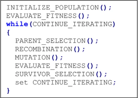
An evolutionary algorithm can be seen not only as an optimization algorithm (in which every new solution is closer to the optimal one), but also as a process of adaptation (the environment selects the best solutions. i.e. the ones that are best adapted to its conditions). In order to measure this, it is absolutely necessary to define what is called fitness function, which gives an idea of how good a solution is. The underlying theory can be expressed as follows: given a fixed population (individuals), a new set of candidates (i.e. possible solutions) is generated from some of the best elements by recombination and/or mutation. Afterwards, the whole population is evaluated in terms of the fitness function, and then the best individuals are allowed to pass to the next generation. The pseudocode of a generic evolutionary algorithm is shown in Table II.1.
Table II.1. Generic evolutionary algorithm pseudocode INITIALIZE_POPULATION();
EVALUATE_FITNESS();
while(CONTINUE_ITERATING) {
PARENT_SELECTION(); RECOMBINATION(); MUTATION();
Evolutionary Computation 23
Fig. II.1. Evolutionary algorithm flowchart
In Fig. II.1, the generic evolutionary algorithm flowchart is shown, emphasizing the iterative process that takes place.
The initialization process is usually random, i.e. the first population is generated randomly. The termination condition can be set according to different criteria: limit of generations reached, fitness variation below user-defined bounds (diversity loss), fitness close to an acceptable value, etc.
II.1
Components
There are some elements that must be taken into account when dealing with evolutionary algorithms. These are the main components:
Representation Fitness function Genetic operators Selection operators
II.1.1
Representation
This is a very important element in any evolutionary algorithm definition. Each individual has to be uniquely defined by its representation. Looking back to the biological systems, an analogy can be established between genotype and representation. Every candidate solution would be determined by a set of genes (the same way phenotype was determined by genotype).
Representation Individual
Genotype Phenotype
1 0 0 1 9
1 0 0 1 -7
Table II.2. Representation examples
Two representation examples have been provided in Table II.2. Although both have the same genotype, the phenotype is completely different. In the first example the
Parent selection Survivor selection
Recombination Mutation
Population
Parents Offspring
genotype encodes an unsigned integer, whereas in the second it is used to encode a two’s complement signed integer. Therefore, it is extremely important to adopt a good representation scheme, as well as to maintain it throughout the whole algorithm, because the rest of the operations will be based on it.
In evolutionary algorithms terminology, the genotype or representation is usually referred to as chromosome, i.e. a set of characteristics (genes) that define the individual.
II.1.2
Fitness Function
The fitness function is also called evaluation function, and it is an expression used to measure the quality of a solution, i.e. how close to the theoretical best achievable solution the current one is.
Given that evolutionary algorithms are often used to solve optimization problems, sometimes the fitness function is referred to as objective function. It is important to keep in mind that the definition of a good fitness function, along with a good representation scheme, is the root of a well-designed and effective evolutionary algorithm. For instance, if the problem is to find the value within an interval whose square value is higher, a good choice for the fitness function would be 𝑓(𝑥) = 𝑥2.
II.1.3
Genetic Operators
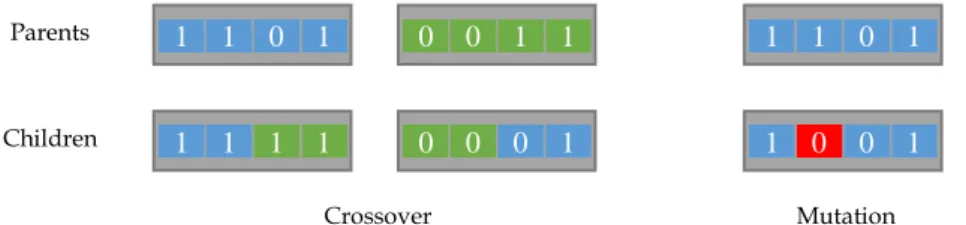
A genetic operator can be defined as a mechanism whose function is to introduce diversity in any given population, generating new candidate solutions. Trying to replicate natural (biological) systems, two different operations have been proposed: on the one hand crossover; on the other hand mutation. The former approach uses two individuals (the so-called parents) and generates two children by recombining genetic characteristics from each parent. Therefore, any children has features inherited from both its parents, and the best genes can be transferred from a generation to the next one. The latter uses only one element to generate a new individual (another child) by changing one or even more of the genetic traits of the parent. With this mechanism new genes, which could provide better adaptation levels, appear.
Fig. II.2. Genetic operators over a binary representation (chromosome)
1 1 0 1 0 0 1 1
1 1 1 1 0 0 0 1
1 1 0 1
1 0 0 1
Parents
Children
Evolutionary Computation 25
Differences between both genetic operators can be seen in Fig. II.2. On the left side, a crossover operation is performed. Note that each child has half the genes from each parent, thus merging their genetic information. However, only one parent is necessary when the genetic operator is mutation, as it is shown on the right side, where only one gene is changed within the whole chromosome (this particular gene has been highlighted in red in order to emphasize the change).
One of the most important characteristics of this genetic operators is randomness, i.e. they are stochastic processes. Mutation has to be a random process in order to introduce only non-biased changes in the population. Crossover depends strongly on random drawings to decide which part of the parents would be recombined and in which way.
Depending on the specific evolutionary algorithm, these genetic operators may or may not appear. It is a task for the designer to choose whether to use crossover, mutation or both operations. Further information regarding the different proposed algorithms would be provided in the following sections.
II.1.4
Selection Operators
In each iteration (generation), two selection processes take place. The first one is used so that the mating pool, i.e. the individuals that would be the parents, can be selected. The second selection process is in charge of discarding those individuals that are not well-suited for the environment in which they are (this takes us back to the concept of natural selection).
Parent selection is usually done using a stochastic process, in order to allow that even weaker individuals can be promoted to the parent status. The reason for this process to be based upon random drawings is simple: it prevents from getting stuck at a local optimum. Therefore, every individual has a chance to become a parent, even though the probabilities are not the same (stronger individuals, i.e. with higher fitness values, are more likely to be chosen than weaker individuals).
As opposed to parent selection (stochastic process), survivor selection is usually a deterministic process. There are a lot of different possible implementations such as ordering the individuals according to their fitness values and selecting as survivors the top segment, or using age criteria: only the children survive, individuals whose fitness is weighted with the number of generations they have been alive, etc.
II.2
Characteristics
Evolutionary algorithms provide us with good problem-solving capabilities. Moreover, the solutions obtained using these techniques are (in most of the cases, but not in all of them) by far better than the ones which could result from a random search, even though evolutionary algorithms are highly dependent on random processes. Evolutionary algorithms are also commonly thought of as generic problem solvers. The same algorithm could be used to solve problems that are not related at all. The reason is simple (and has already been explained): the actual solutions (phenotype) are encoded in each chromosome (genotype). Therefore, if two non-related problems can be expressed using the same representation and their fitness can be evaluated in terms of the same fitness function, the algorithm is well-suited for both computations. However, these algorithms have a drawback that is worth noticing: the more generic the problem solver is (i.e. the wider the range of problems it can be applied to), the worse the solutions are. This means that evolutionary algorithms would lead to good solutions, but specific problem solvers would end up finding better results. Therefore, a tradeoff between the number of problems the algorithm can solve and the quality of the solutions appears. This tradeoff is shown in Fig. II.3. Nevertheless, decreases in the quality of the solution caused by evolutionary computing are negligible comparing with the flexibility it entails, and this is the reason why evolutionary computing is widely spread nowadays.
Fig. II.3. Comparison between different problem-solving algorithms
How does an evolutionary algorithm work? Generally speaking, the working cycle of any of the different approaches consists of two stages. In the first stage, the algorithm searches the solution space, starting from the random initialization values. Once the algorithm has found what could be considered as a good solution, the second stage starts. In this step, the algorithm tries to improve the current solution. These two stages are clearly differentiated if analyzed on a time vs. improvement basis. The first stage
Aver
ag
e s
ol
ut
io
n
qu
al
ity
Problem range Evolutionary algorithm
Random search
Evolutionary Computation 27
shows large variations in fitness values in a few generations, whereas in the second stage the changes are almost insignificant. This temporal analysis becomes particularly useful when defining some termination conditions, e.g. a good termination condition based on the execution time would be to stop when the optimization process has reached this second stage.
Fig. II.4. Fitness evolution vs. number of generations
Fig. II.4 shows a real example of an optimization process using a genetic algorithm. There is a huge increase in the fitness value from generation #1200 to approximately generation #2000. This corresponds to the aforementioned first stage of the evolutionary search. After generation #2000, the algorithm seems to stop its search (the fitness gets stuck in a plateau, especially after generation #5000), due to the fact that better solutions are more and more unlikely to appear.
II.3
Genetic Algorithms
Genetic algorithms are said to be the most extended form of evolutionary algorithms. Commonly used in optimization problems, these algorithms use numeric strings as representation, usually in the form of binary or integer arrays. Although both crossover and mutation are used, the former is the main operator. The parent selection scheme uses a fitness-biased random approach. On the contrary, the survivor selection scheme is usually generational (only the offspring survives, thus replacing the whole previous population) or deterministic (always taking into account fitness criteria).
II.4
Evolution Strategies
Evolution strategies try to take advantage of a very important feature: self-adaptive capabilities. In order to achieve this goal, some algorithmic parameters are evolved along with the solutions (these parameters could even be included as part of the genes that constitute a chromosome). Each chromosome is usually represented as an array of real numbers. Evolution is mutation-based in almost every case, but recombination can also appear as intermediate recombination (i.e. averaging the genes of the parents), or discrete recombination (i.e. selecting randomly as a child one of the parents). Each individual within the population has the same likelihood of being selected as a parent (no fitness-biased criteria appear in this approach), and the surviving population can be generated (always as a deterministic process) using only the offspring or including the previous population to the offspring. The former strategy seems to provide better results, because it avoids the memory effect, allowing transitions from local optima.
II.5
Evolutionary Programming
Evolutionary programming is really useful when the target problem is to optimize a fixed program structure which has some parameters that can be changed. Originally developed to generate artificial intelligence (emulating learning processes), evolutionary programming considers adaptation and environment prediction must-have features. This algorithm is only based on mutation, generating one child from each of the individuals, i.e. every individual is considered a parent. Survivors are selected randomly from the initial population plus the offspring.
Evolutionary Computation 29
II.6
Genetic Programming
Also focused on program optimization, the main difference between evolutionary programming and genetic programming is that the latter represents each program as a tree and changes its whole structure (as opposed to the former, in which only some parameters were changed). Both genetic operators can be used in order to modify branches in the trees (recombining by swapping, or mutating by adding or deleting some of the leaves). Parent selection follows the same scheme as in genetic algorithms (fitness-biased random selection), and survivors are selected using generational criteria (i.e. only the offspring survives).
Fig. II.5. Genetic programming representation: tree structure
In Fig. II.5, a typical chromosome in genetic programming is shown. The genotype encodes the function 𝑓(𝑥, 𝑦) = (10−𝑦6 ) + (5 ∙ sin (𝑥)).
II.7
Other Approaches
Evolutionary computing has been a developing field ever since it appeared. There is a vast range of different implementations and algorithms, but for the sake of convenience only a few of them will be presented here.
When dealing with complex problems which can be divided in simpler subproblems, memetic algorithms may be a wise choice. These algorithms are hybrid, for they combine evolutionary processes and problem-solving knowledge (heuristics). Given that a new component is introduced, a new stage is also necessary: the learning stage, in which the algorithm gathers every piece of knowledge that is available. Memetic algorithms can be found in the literature as hybrid genetic algorithms, Baldwinian evolutionary algorithms or Lamarckian evolutionary algorithms, but all of them have in common the addition of one or more local search (i.e. better solutions in the neighborhood of a known one) stages to the traditional evolutionary algorithm.
+
6 /
- 5
*
sin
y
Coevolution seems to be the most appealing concept regarding evolutionary computing, and can be implemented as a cooperative algorithm or as a competitive algorithm. Either it is one or the other, the population has different species. In cooperative coevolution, each species represents a part of the problem and cooperate in order to come with a solution of a larger problem. As opposed to that, competitive coevolution is based on individuals gaining fitness at each other’s expense, i.e. the species fight against each other.
The last example of evolutionary computation techniques is called interactive evolution, and turns out to be very useful when dealing with problems in which there is no such thing as a clearly defined fitness function. Subjective opinions have a strong influence in the selection process. Therefore, biased external interference is what best defines interactive evolution, even though this interference might or might not be direct (e.g. deciding whether an individual can survive or not).
III.
Current Research Lines
Evolutionary computation is an enormous research field. Therefore, we would only present those works closely related to particle filtering (i.e. particle filters which have been enhanced with evolutionary computing).
Particle filtering and evolutionary algorithms, especially genetic algorithms, have conceptual similarities. These similarities have been studied and documented for a long time. For instance, in [2] a modified particle filter is presented. The author uses genetic operators such as crossover and mutation to implement the prediction stage of the filter, describing the whole algorithmic implementation of what he calls Genetic Algorithm Filter. The connection between particle filtering (Monte Carlo simulations) and Bayesian inference and their application to evolutionary environments has also been studied. In [3], the foundations for Bayesian evolutionary computation are presented. The idea is to guide the evolutionary process using Bayes’ rule, since it is stated in the paper that the most probable solution could be considered the best one. However, this is not state-of-the-art research.
Evolutionary Computation 31
introducing genetic operators right after performing the importance sampling stage and immediately before the resampling stage, which uses a parameter (effective number of particles) in order to decide whether to perform resampling or not. In this paper it is also shown that the mutation operator provides better dynamic response when the state jumps abruptly.
Other research lines use parallel distributed filters, i.e. with several subpopulations evolving at the same time. In [5], the authors use these subpopulations to perform genetic operations and, from time to time, migrate the best individuals from one subpopulation to the others so that the best genetic traits can be shared. This also leads to an improvement in global optimum search. Moreover, the concept of genetic resampling stage is introduced in this paper for the first time. Nevertheless, the paper provides only simulation results.
More complex examples can also be found in the literature: a hybrid evolutionary particle filter is presented in [6]. This hybrid approach tries to take advantage of both genetic algorithms (to maintain particle diversity) and particle swarm optimization (to optimize the final particle distribution). Furthermore, the algorithm presented has parallel features, thus reducing computation times. The strategy presented divides the population in two groups, and then performs the specific operations that are required: in one group, a genetic algorithm; in the other, particle swarm optimization. Before the next time step, a migration operation is performed (to share genetic information, as in previous examples).
Real-world applications include object tracking, as in [7]. Another evolutionary approach is presented in order to deal with sample impoverishment. In this case, the evolutionary resampling stage may or may not take part in the estimation loop. The decision is made based on the aforementioned parameter, i.e. the effective number of particles. The algorithm presented provides good results but it is not accurate in occlusion tracking sequences.
Recent studies with differential evolution have been conducted in order to reduce significantly sample sizes [8]. The differential evolution algorithm divides the particles in three different groups: the first group would undergo crossover; the second group would undergo mutation; the last group would not suffer any modification. One important fact about this work is that the evolutionary stage takes place at the very beginning of the process, and it is immediately followed by the importance sampling stage.
IV.
References
[1] Turing, A.: Intelligent Machinery. In: D. Ince (ed.) Collected Works of A. M. Turing: Mechanical Intelligence. Elsevier Science (1992)
[2] T. Higuchi, “Monte Carlo filter using the genetic algorithm operators,” Journal of Statistical Computation and Simulation, vol. 59, pp. 1-23, 1997
[3] Byoung-Tak Zhang, "A Bayesian framework for evolutionary computation," Evolutionary Computation, 1999. CEC 99. Proceedings of the 1999 Congress on , vol.1, no., pp.,728 Vol. 1, 1999
[4] Seongkeun Park; Jae Pil Hwang; Euntai Kim; Hyung-Jin Kang, "A New Evolutionary Particle Filter for the Prevention of Sample Impoverishment," Evolutionary Computation, IEEE Transactions on , vol.13, no.4, pp.801,809, Aug. 2009
[5] Cong Li; Qin Honglei; Xing Juhong, "Distributed genetic resampling particle filter," Advanced Computer Theory and Engineering (ICACTE), 2010 3rd International Conference on , vol.2, no., pp.V2-32,V2-37, 20-22 Aug. 2010 [6] Jialong Zhang; Tien-Szu Pan; Jeng-Shyang Pan, "A Parallel Hybrid
Evolutionary Particle Filter for Nonlinear State Estimation," Robot, Vision and Signal Processing (RVSP), 2011 First International Conference on , vol., no., pp.308,312, 21-23 Nov. 2011
[7] Wei Leong Khong; Wei Yeang Kow; Yit Kwong Chin; Mei Yeen Choong; Teo, K.T.K., "Enhancement of Particle Filter Resampling in Vehicle Tracking Via Genetic Algorithm," Computer Modeling and Simulation (EMS), 2012 Sixth UKSim/AMSS European Symposium on , vol., no., pp.243,248, 14-16 Nov. 2012 [8] Nyirarugira, C.; Tae Yong Kim, "Adaptive evolutional strategy of particle
Evolutionary Particle Filter 33
Evolutionary Particle Filter
I.
Introduction
In this chapter, the proposed architecture is presented. The Evolutionary Particle Filter has been designed for movement estimation applications. In this application, the state variables are four: x-axis position, y-axis position, x-axis velocity and y-axis velocity.
Fig. I.1. State variables
As far as this implementation is concerned, it has been assumed that the movement does not have any acceleration at all. The only allowed changes in both velocity components are the ones caused by the addition of random noise. The motion equations can be then expressed as follows:
{
𝑥𝑘= 𝑥𝑘−1+ 𝑇 ∙ 𝑣𝑥𝑘−1+ 𝑤𝑘𝑥 𝑦𝑘 = 𝑦𝑘−1+ 𝑇 ∙ 𝑣𝑦𝑘−1+ 𝑤𝑘𝑦
𝑣𝑥𝑘= 𝑣𝑥𝑘−1+ 𝑤𝑘𝑣𝑥 𝑣𝑦𝑘= 𝑣𝑦𝑘−1+ 𝑤𝑘𝑣𝑦
This motion model can also be expressed in matrix-based notation: 𝒙𝒌= 𝐴 ∙ 𝒙𝒌−𝟏+ 𝒘𝒌−𝟏
𝐴 = [
1 0 𝑇 0 0 1 0 𝑇 0 0 1 0 0 0 0 1
] 𝒙𝒌 = [ 𝑥𝑘 𝑦𝑘 𝑣𝑥𝑘 𝑣𝑦𝑘 ] 𝒘𝒌= [ 𝑤𝑘𝑥 𝑤𝑘𝑦 𝑤𝑘𝑣𝑥 𝑤𝑘𝑣𝑦] ~ [ 𝑁(𝜇𝑥, 𝜎𝑥) 𝑁 𝜇𝑦, 𝜎𝑦 𝑁(𝜇𝑣𝑥, 𝜎𝑣𝑥) 𝑁 𝜇𝑣𝑦, 𝜎𝑣𝑦 ]
As opposed to [1], this model does not perform any estimations regarding the current velocity in each axis. Therefore, a significant reduction in terms of memory resources is achieved, since it is no longer necessary to store previous position values.
However, the state space is not observable. The only state variables that are measurable are both x-axis and y-axis positions. Therefore, the measurement model can be represented (in matrix notation) as:
𝒛𝒌= 𝐻 ∙ 𝒙𝒌
𝐻 = [1 0 0 00 1 0 0] 𝒛𝒌= [𝑧𝑥𝑧𝑦𝑘 𝑘]
The most important advantage this proposal has is that it is highly application-independent. This estimation engine can be used to track a wide range of different elements, as long as their state can be expressed as the aforementioned 𝒙𝒌 array. This feature makes the system incredibly suitable for a reconfigurable platform. By using different (reconfigurable) preprocessing stages, the Evolutionary Particle Filter can track colored objects, corners, shapes, etc.
Fig. I.2. Evolutionary Particle Filter flowchart
The modified flowchart of the Evolutionary Particle Filter is shown in Fig. I.2. Note that this flowchart is based on the basic particle filter but adding an extra stage, which is in charge of performing resampling using an evolutionary algorithm.
The rest of this chapter is organized as follows: first, the algorithmic implementation of the evolutionary resampling stage will be presented and discussed. Then, the hardware-based modules will be explained in detail.
Initialization
Importance Sampling
Evolutionary Resampling
Weight calculation
Process Model
Measurement Model +
Actual Measurement
Evolutionary Particle Filter 35
II.
Evolutionary Resampling Stage
Placed right after the Importance Sampling process, i.e. the process model update, and immediately before weight calculation and state estimation, the evolutionary resampling stage constitutes itself the distinctive element of the EPF algorithm. Although some approaches can be found in the literature (as in the aforementioned proposal of [2]), some modifications have been introduced and will be discussed in the forthcoming paragraphs.
A genetic algorithm has been selected, due to the flexibility of introducing both genetic operators (crossover and mutation) and to the fact that chromosomes will be represented as integer arrays. The target application has some timing constraints (e.g. frames per second in the camera); therefore, the termination condition is set to be reaching a fixed number of generations.
II.1
Crossover
Arithmetic crossover will be used as recombination operator. Crossover takes place whenever a random number 𝑝~𝑈(0,1) satisfies 𝑝 < 𝑝𝑐, being 𝑝𝑐 the crossover probability. Arithmetic crossover can be expressed in terms of the following equations:
{𝑥𝑘𝑎= 𝛼 ∙ 𝑥𝑘𝑖 + (1 − 𝛼) ∙ 𝑥𝑘𝑗 𝑥𝑘𝑏= 𝛼 ∙ 𝑥𝑘𝑗+ (1 − 𝛼) ∙ 𝑥𝑘𝑖
where 𝑥𝑘𝑎 and 𝑥𝑘𝑏 are the children, i.e. the offspring, and can be obtained weighting the states of the parents 𝑥𝑘𝑖 and 𝑥𝑘𝑗. The subscripts (k) represent the current time step in which the system is, whereas the superscripts are the individual identifiers (a, b for the children; i, j for the parents). The weight factor is a random number drawn from a uniform distribution 𝛼~𝑈(0,1).
II.2
Mutation
Mutations should occur whenever a random number 𝑝~𝑈(0,1) satisfies 𝑝 < 𝑝𝑚, being 𝑝𝑚 the mutation probability. In this proposal, two mutation operations can be performed. If 𝑝 ≥ 𝑝𝑚∙ 𝑟𝑚, with 𝑟𝑚=
𝑝𝑟𝑎𝑛𝑑𝑜𝑚 𝑝𝑙𝑎𝑐𝑒𝑚𝑒𝑛𝑡
𝑝𝑙𝑜𝑐𝑎𝑙 𝑠𝑒𝑎𝑟𝑐ℎ being the mutation ratio, a local search mutation operator is used. Otherwise, the mutation operator generates a random child over the whole search space.
Local search mutation adds Gaussian noise, i.e. random numbers, to the parents’ state variables, as can be seen in the following equation:
𝑥𝑘𝑐= 𝑥𝑘𝑖 + 𝛿𝑘
𝑥𝑘𝑐= 𝑥𝑚𝑖𝑛+ 𝛽 ∙ (𝑥𝑚𝑎𝑥− 𝑥𝑚𝑖𝑛)
In these expressions 𝑥𝑘𝑐 is the child, 𝑥𝑘𝑖 the parent (only in local search mutation), 𝛿𝑘~𝑁(𝜇, 𝜎) (only in local search mutation), 𝑥𝑚𝑖𝑛 and 𝑥𝑚𝑎𝑥 the limits of the search space (only in random placement mutation), and 𝛽~𝑈(0,1) (only in random placement mutation).
Each of these two mutation operations has a defined purpose. On the one hand, local search helps reaching close optimal points. On the other hand, random placement promotes global optimization (not just local), making possible for the population to jump to unexplored regions in the state space and evolve there. Hence, better solutions might be obtained.
II.3
Selection
The chosen selection algorithm is the so-called Stochastic Universal Sampling (SUS). This algorithm appears as a development of Fitness Proportionate Selection (FPS), also known as roulette wheel algorithm, even though the drawing of random numbers is carried out in a different manner. Considering that 𝑛𝑠𝑒𝑙 elements have to be selected, FPS draws 𝑛𝑠𝑒𝑙 different uniform random numbers, whereas SUS only draws one using a uniform distribution.
𝑟~𝑈 (0,∑ 𝑓𝑖 𝑖 𝑛𝑠𝑒𝑙)
In the last expression, 𝑓𝑖 is the fitness value of the individual 𝑥𝑘𝑖, 𝑛𝑠𝑒𝑙 is the number of individuals that have to be selected, and 𝑟 is the value which is drawn.
How does Stochastic Universal Sampling work? First, individuals have to be sorted according to their fitness value.
𝑓 = [𝑓𝑛−1 𝑓𝑛−2 ⋯ 𝑓1 𝑓0] 𝑓0≥ 𝑓1≥ ⋯ ≥ 𝑓𝑛−2≥ 𝑓𝑛−1
Then, the cumulative fitness vector is computed starting with the individual that has the highest fitness value.
𝑞𝑘= ∑ 𝑓𝑖 𝑘
𝑖=0
Once the random number 𝑟 has been drawn, the individual k is selected if 𝑟 < 𝑞𝑘. Otherwise, 𝑟 is incremented as follows:
Evolutionary Particle Filter 37
Fig. II.1. Stochastic universal sampling
Therefore, the idea is that every selected individual is equidistant with the previous and the following element. A good example has been provided in Fig. II.1, where 𝑛𝑠𝑒𝑙 = 7. The first element is selected using the random number 𝑟, and then the following elements are obtained adding a fixed increment, which depends on both the number of desired selected individuals and the maximum value of the cumulative fitness vector. In this particular example, the seven selected individuals are [𝑥0, 𝑥0, 𝑥1, 𝑥1, 𝑥2, 𝑥3, 𝑥5]. This selection algorithm has very important features, such as being unbiased. However, the most important characteristic is that with this selection strategy, even the weakest members of the population can be selected, as in the previous example. This also prevents the evolutionary process from remaining stuck at a local maximum.
Table II.1. Example code for Stochastic Universal Sampling selection
x0 x1 x2 x3 x4 x5
0 ∑ 𝑓𝑖
𝑖
∑ 𝑓𝑖 𝑖 𝑛𝑠𝑒𝑙 𝑟 ∈ 0,∑ 𝑓𝑖 𝑖
𝑛𝑠𝑒𝑙)
i = 0; j = 0;
inc = q[N-1]/N_SEL;
r = inc*(rand()/RAND_MAX); while(i<N_SEL)
{
if(r<=q[j]) {
selected[i] = j; r += inc;
i++; }
This selection scheme has been adopted in this work as both parent and survivor selection algorithm. The main reason for this decision is that implementing more than one selection algorithm might increase significantly resource utilization rates. Therefore, survivor selection will be stochastic in this proposal, rather than deterministic as in many examples in the literature.
To summarize, the proposed evolutionary algorithm is a genetic algorithm with Stochastic Universal Sampling selection, arithmetic recombination and both local and global mutation schemes, and its flowchart can be seen in Fig. II.2.
Fig. II.2. Evolutionary resampling flowchart
III.
Hardware Architecture
The Evolutionary Particle Filter has been implemented as an IP (Intellectual Property) core, i.e. a hardware module. A modular approach has been adopted so as to make the design stage easier and to favor reusability. Moreover, it could allow future reconfiguration within the core itself.
YES NO
END?
Parent selection Stochastic Universal Sampling
Survivor selection Stochastic Universal Sampling
Mutation 𝑥𝑘𝑐 = 𝑥𝑚𝑖𝑛+ 𝛽 ∙ (𝑥𝑚𝑎𝑥− 𝑥𝑚𝑖𝑛) 𝛽~𝑈(0,1)
𝑥𝑘𝑐= 𝑥𝑘𝑖 + 𝛿𝑘 𝛿𝑘~𝑁(𝜇, 𝜎) Random placement Local search
Crossover
{𝑥𝑘 𝑎= 𝛼 ∙ 𝑥
𝑘𝑖 + (1 − 𝛼) ∙ 𝑥𝑘𝑗 𝑥𝑘𝑏= 𝛼 ∙ 𝑥𝑘𝑗+ (1 − 𝛼) ∙ 𝑥𝑘𝑖
Evolutionary Particle Filter 39
Fig. III.1. Evolutionary Particle Filter block diagram
The proposed modular architecture can be seen in Fig. III.1. Some control signals and data connections have been simplified in the diagram in order to avoid excessive complexity. The signals highlighted in red represent the external connections of the hardware module, i.e. the interface with the top system. The main modules of the Evolutionary Particle Filter system are:
Random number generator. Fitness calculation.
Particle registers. Process model. Crossover unit. Mutation unit. Dividers. Control logic.
Divider #1
Divider #2
Control Logic
Random Number Generator
Process Model
Mutation Unit Crossover
Unit Calculation Fitness
Main Particle Register
These blocks will be presented in detail in the forthcoming sections of this chapter. Hardware designs have some limitations in terms of arithmetic operations. Designers have to decide whether to use integer, fixed-point or even floating-point arithmetic. There is an obvious tradeoff between precision and resource consumption (or time): the more precise the operations have to be, the more complex the resulting system is. Focusing on the Evolutionary Particle Filter, it seems clear that estimation and prediction tasks require accurate computations, at least to some extent. However, extra complexity in the design is not desirable. For this reason, fixed-point arithmetic has been selected as the most convenient implementation strategy in this thesis.
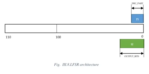
Fixed-point arithmetic uses real number representations in which the decimal part, i.e. those digits after the radix point, and the integer part have a fixed size. For instance, in Fig. III.2, 𝑛𝑑 would represent the size, in bits, of the decimal part, and 𝑛𝑖 would represent the size of the integer part.
Fig. III.2. Fixed-point number representation
Having a fixed number of bits for both integer and decimal part generates some problems. The first problem a designer might face is overflow or underflow phenomena, which occur when the result of an operation cannot be represented with the given resolution, i.e. the number of bits, the system has. For example, the result of 24 + 12 with an unsigned integer resolution of 5 bits would be 4 instead of 36. Another important problem of using fixed-point arithmetic is that not all the numbers within an interval can be represented, since the less significant bit determines the minimum increment. Therefore, the resolution is finite. For example, if the decimal part resolution were 4 bits, the minimum increment would be 0.625.
In this design, numbers are represented as 19-bit integers, unless otherwise specified: 8-bit decimal part, 10-bit integer part and 1 bit to represent the sign (2’s complement). This gives an overall representation range from -1024.0 to 1023.99609375.
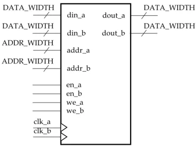
III.1
Random Number Generator
Stochastic processes play a very important role in the Evolutionary Particle Filter. On the one hand, normal-distributed random numbers are used in some stages (e.g. process model update, or importance sampling). On the other hand, the evolutionary algorithm uses uniform random numbers to decide whether to perform a genetic operation or not. Therefore, the random number generator is an essential part of the design.