A Wavelet neural network for detection of signals in communications

ReMake by the authors of 1998 SPIE original

A Wavelet neural network for detection of signals in communications

Raquel Gómez-Sánchez

, Diego Andina

a

Grupo de Automatización en Señal y Comunicaciones

Universidad Politécnica de Madrid

Ciudad Universitaria s/n, 28040 Madrid

ABSTRACT

Our objective is the design and simulation of an efficient system for detection of signals in communications in terms of speed and computational complexity. The proposed scheme takes advantage of two powerful frameworks in signal processing: Wavelets and Neural Networks. The decision system will take a decision based on the computation of the a priori probabilities of the input signal. For the estimation of such probability density functions, a Wavelet Neural Network (WNN) has been chosen. The election has arosen under the following considerations: (a) neural networks have been established as a general approximation tool for fitting nonlinear models from input/output data and (b) the increasing popularity of the wavelet decomposition as a powerful tool for approximation. The integration of the above factors leads to the wavelet neural network concept. This network preserve the universal approximation property of wavelet series, with the advantage of the speed and efficient computation of a neural network architecture. The topology and learning algorithm of the network will provide an efficient approximation to the required probability density functions.

Keywords: detection, communications, wavelets, neural networks, a priori probabilities, nonlinear models.

1. INTRODUCTION

Wavelet theory has emerged as a powerful tool in many areas of engineering and applied mathematics, as signal processing and numerical analysis. Its application range from constituting relevant theoretical models1 to providing efficient mechanisms for implementations in one and two dimensions, through Quadrature Mirror Filter banks2 (QMF banks structures).

However, the filter bank implementations of wavelet bases suffers from the lack of adaptability. QMF banks provide decompositions for all functions in the associated subspace3. When the objective is to approximate a single function, many wavelets in the subspace basis could be probably eliminated for a more efficient representation. Another disadvantage is that QMF banks provide decompositions just over orthogonal wavelet bases, while nonorthogonal bases, easier to implement, could be sufficient.

An alternative for constructing wavelet basis arises from the neural network concept4. Many studies have shown the ability of neural networks for approximating functions5. In its analytical expression, a neural network transfer function appears as a signal decomposition in terms of the activation function. When a wavelet is used for the nodes, the resulting network has been denominated Wavelet Neural Network6.

Wavelet Neural Networks (WNN) constitute a recent topic in signal processing and neural networks areas. His goal consists on combining wavelet properties and neural network structures to determine the net parameters which best approximate a given function. Several ways have been proposed to approach the design of wavelet neural networks. In 6 wavelet network is introduced as a class of feedforward networks composed of wavelets, in 7 the Discrete Wavelet Transform is used for analyzing and synthesizing feedforward neural networks, and in 8 orthonormal wavelet bases are used for constructing wavelet-based neural networks.

*

This paper is based on one of the most recent works about the topic9, where algorithms for wavelet network construction are proposed. In the following section, a brief introduction to wavelet theory is presented. Results of wavelet neural networks implementation, when applied to the problem of function approximation, are reported in Section 3. In section 4, these implementations are applied to the problem of signal detection in communications. Finally, conclusions will be drawn in Section 5.

2. WAVELET BASES FOR APPROXIMATION

The problem of approximating a function in the Hilbert space L2(ℜ) has been classically solved by orthonormal Fourier bases of the type {an ejωnt , ωn∈ℜ, an∈C}, where the function decomposition coefficients, an, supply information about frequency

content. But in many cases it would be desirable that the coefficients supply information about both, time and frequency content. It is well known10 Fourier series only appears non-localized frequency information. In order to obtain time-frequency localization, alternative transformations have been developed, such the Short-Time-Fourier-Transform11, and Continuous and Discrete Wavelet Transforms1. Below a brief resume of the elemental theory for approximating functions with wavelets is presented.

1) Unidimensional case. It can be shown12 that, adequately selectingα and β, the family of functions:

(1)

{

}

Ψ = ψm n =α ψ α −β ∈ α ∈ℜ β∈ℜ

m m

x x n m n Z

,

/

( ) 2 ( ): , , +,

under the admisibility condition for a function in L2(ℜ), ψ: ℜ→ℜ:

Cψ d

ω

ω ω

=

∞

∫

0

< ∞ (2)

constitutes a frame, that is, a natural generalization of orthonormal bases for Hilbert spaces, which leads to decompositions of signals in terms of functions that have less requirements than orthonormal bases. Moreover, if ψ satisfies further conditions12, the family (2) constitutes an orthogonal basis.

When the condition (2) is satisfied, the function ψ is said to be a mother wavelet. If the further conditions for orthogonality are required, the mother wavelet constitutes an orthogonal mother wavelet. For the problem of function approximation, a frame suffices, so that the conditions on the mother wavelet can be relaxed and much more freedom on the choice of the wavelet function is gained. Nevertheless, the fast algorithms associated with orthonormal wavelet bases are lost.

Then, given any f∈ L2(ℜ), it can be decomposed in term of the frame elements (1) as:

f c_{m n m n} m n

=

∑

,

ψ (3)

Under certain conditions on the parametersα and β, the family (1) may be a tight frame7, so that the coefficients cm,n can be

computed as the usual Fourier coefficients. Then the problem of representing a function f lies on computing the frame coefficients in (3).

2) Extension to multidimensional wavelets. In the Hilbert space L2(ℜn), a mother wavelet can be obtained as follows:

ψ( )x =ψ_s(x ) ψ_s(x_n),x n

1 K ∈ℜ (4)

where ψs is a mother wavelet in L2(ℜ). The correspondent frame appears as:

{

}

Ψ = det(Dk) / (D xk −tk):tk ∈ ℜ ,D = diag d( ),d ∈ ℜ ,k ∈Z

n

k k k

n

1 2ψ ₍₅₎

For a simpler structure in the multidimensional case, usually radial wavelets functions13 are used. A radial wavelet in L2(ℜn) satisfies:

(x)= g( x ) (6)

ψ

where g: ℜ→ℜ is a single variable function and ||.|| represents the vector norm. The radial wavelets frames are naturally single-scaling, so then, structurally simpler than multiscaling wavelet frames, as (5).

A function f ∈ L2(ℜn) can be decomposed in terms of a multidimensional frame in the way it was done for the unidimensional case, shown in (3). Now, the computation of the scalar products is significatively more expensive, due to the higher dimensionality of the problem.

3. WAVELET NETWORKS

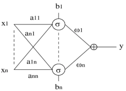
Neural networks are a class of computationalarchitectures which are composed of interconnected, simple processing nodes with weighted interconnections. Figure 1 shows a simple neural network, known as (1+1/2)-layer neural network6.

x1

xn

b1

bn a11

a1n an1

ann

ω1

ωn

y

σ

σ

Figure 1: The (1+1/2)-layer neural network.

This network only differs to the traditional 2-layer neural network in the absence of the output node. The transfer function of the network in the figure can be analytically described as follows:

y f x wi ai x b a x b w

T

i i

n

i

i i

= = + ∈ ℜ ∈

=

∑

( ) σ( ), , , ,

1

n

ℜ (7)

which reminds of an expansion in terms of the functions:

{

}

i: i( )x (ai x bi) (8)

For the unidimensional case and being σ a mother wavelet, expression (7) results identical to a decomposition in terms of a truncated wavelet frame. In such case, network in Figure 1 is called wavelet neural network.

For the unidimensional case, the wavelet neural network implements a truncated version of the frame in (1), being the translation parameters βn=bithe offsets and the scale parameters αk=akthe weights from the input to the neurons7. In the

wavelet frame, for each translation parameter, infinite scales parameters (resolution levels) are considered. In the truncated frame, a number J of resolution levels is selected. This means that the number of wavelets in the truncated frame (nodes in the network) corresponds to J×P, being P the number of the selected translation parameters. As a result, the offsets of the nodes are repeated J times.

Several training algorithms have been proposed and developed for networks like Figure 1. The backpropagation

under these training algorithms. However, these methods do not naturally give rise to systematic synthesis procedures for these networks.

With the interpretation in (7) as a wavelet frame decomposition, an explicit link between the network coefficients and some appropriate transform is provided. This may be extremely useful for achieving the optimal structure (number of nodes), and guaranties the universal approximation property.

Several works have appeared on the topic of constructing wavelet neural networks. One of the most recent works9 in which this paper is based, propose algorithms to approach the problem of nonparametric regression estimation, and will be summarized below.

Two random variables x∈ℜn and y∈ℜ satisfy a regression model, when they are related as follows:

y= f x( )+e (9)

where f is a nonlinear function belonging to some functional space, and e is a white noise independent of x. The variables x and

y are referred as the input and output model respectively.

A training data set is defined as a sample set of the input-output pair (x,y):

{

}

X = x x, ,x

{

}

Y y y y

n

n =

1 2

1, 2, , K

K (10)

The problem to be solved is to find a nonparametric estimator fe of f based on the data sample (X,Y). With this information, a

truncated wavelet frame must be selected and the correspondent decomposition coefficients obtained, in order to determine a wavelet neural network structure which fits f.

For the unidimensional case, the first problem addressed above consists on selecting the finite number of elements in the family (1) which best approximate the data. The starting point is a regular wavelet lattice, as shown in Figure 2.

xmin xmax

x

ω

Figure 2: A regular wavelet lattice in the time-frequency plane.

Many wavelets in this regular lattice will probably not contain any data point in their supports. The training data do not provide any information for determining the coefficients of these “empty” wavelets. These wavelets are thus superfluous for the regression estimation problem and should be eliminated.

Once selected the coefficients bi which must appear in the decomposition, attention must be paid to coefficients ak.

Due to the scaling property, increasing the number of parameters ak results in increasing the resolution of the approximation

for a given temporal coefficient bi . In most cases 4 or 5 resolution levels have shown to be sufficient for fitting the training

data set.

(11)

{

S= ψ_i( ),x i=1 2, ,_K,L

}

i L

⎡ ⎤

being L≤ n (some nodes can be eliminated in the training network algorithm). The remaining problem is to find the coefficients wi which define the resultant wavelet neural network:

(12)

f_e x w_i x

i

( )= ( )

=

∑

1

One of the algorithms proposed to find these coefficients is known as stepwise selection by orthogonalization9. In the first step selects the wavelet (node) in S that best fits the observed data, then repeatedly selects the wavelet in the remainder of

S that best fits the data while combining with the previously selected wavelets. For computational efficiency, later selected wavelets are orthonormalized to earlier selected ones.

The following vectorial notations are defined:

(13)

v k

x

x

j

j

j n

= ⎣ ⎢ ⎢

⎢ _⎦

⎥ ⎥ ⎥ ψ

ψ

( )

( )

1 K

where ψj∈ S, j=1,...L, xk∈X. The k constant is a scalar so that vj has unity norm,

(14)

y y

y_n

= ⎡

⎣ ⎢ ⎢ ⎢

⎤

⎦ ⎥ ⎥ ⎥

1 K

being yk ∈Y. At iteration i, li denote the index of the selected wavelet from S. If i is the current iteration number, then vl1, .... vli-1 have been selected in the previous iterations. Let l1= arg maxi (viT y), denote ql1= vl1. The Gram-Schmidt procedure is

used for the following orthogonalization:

p v v q q

q p

p

j j j l l

j j

j

=

( 1) 1, j l1 T

= − ≠

(15)

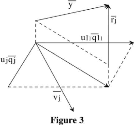
Figure 3 shows that ||rj ||2will be minimized if uj2 = (yTqj )2 is maximized. This leads to the criterion for the selection

of the best wavelet in each step of the algorithm.

ujqj

vj

ul1ql1 y

rj

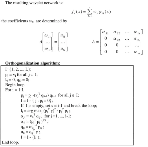
The resulting wavelet network is:

(16)

fe x wli x

i ( )= ( ) =

∑

where the coefficients wli are determined by

(17) A u u A l ls l ls s s ss ω ω α α α 1 1

11 12 1

22 2 0 0 0 0 0 K K K K K K K ⎡ ⎣ ⎢ ⎢ ⎢ ⎤ ⎦ ⎥ ⎥ ⎥ = ⎡ ⎣ ⎢ ⎢ ⎢ ⎤ ⎦ ⎥ ⎥ ⎥ = ⎣ ⎢ ⎢ ⎢ ⎢ ⎦ ⎥ ⎥ ⎥ ⎥ Orthogonalization algorithm: I={1, 2, ..., L};

pj = vj for all j ∈ I; l0 = 0, ql0 = 0; Begin loop For i = 1:L

pj = pj -(vjT qli-1) qli-1 for all j ∈ I; I = I - { j : pj = 0};

If I is empty, set s = i-1 and break the loop; li = arg maxj (pjT y)2 / pjT pj ;

αji = vliT qlj , for j =1, ..., i-1; αii = (pjT pj )1/2 ;

qlj = αii-1 pli ; uli = qljT y ; I = I - {li}; End loop.

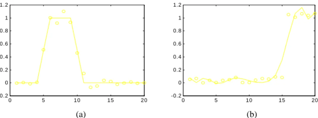
In the figures below several results for different functions approximation using the described algorithm are depicted.

0 5 1 0 1 5 2 0 2 . 8

3 3 . 2 3 . 4 3 . 6 3 . 8 4 4 . 2

0 5 1 0 1 5 2 0 2 . 8

3 3 . 2 3 . 4 3 . 6 3 . 8 4

(a) (b)

0 5 10 15 20 -0.2

0 0.2 0.4 0.6 0.8 1 1.2

0 5 10 15 20

-0.2 0 0.2 0.4 0.6 0.8 1 1.2

(a) (b)

Figure 5: Approximation curves. Noisy approximated function (dot line) and wavelet neural network output (solid line) for uniform noise and variances (a) σ2 = 0.1 and (b) σ2 = 0.01.

4. SIGNAL DETECTION IN COMMUNICATIONS

This section concerns the problem of signal detection in digital communication systems. The interest will be focused in the approximation to the demodulator decision problem by means of a wavelet neural network. A conventional digital communication system15 is shown in Figure 6:

SOURCE ENCODE

CHANNEL

ENCODE MODULATE

INFORMATION SOURCE

C H A N N E L

DEMODULATE SOURCE

DECODE

CHANNEL DECODE INFORMATION

SINK

CHANNEL BITS

si (t)

n(t)

CHANNEL BITS

A

B

Figure 6: Digital communication system scheme.

The subject of study is constituted by the portion between A and B points. One element of a set of 2k symbols, {si(t), i=1, ..., M=2k}, is being transmitted during a symbol interval Ts. The channel attenuates the signal amplitude, and a white noise is added at the input to the demodulator. Therefore, supposed si to be the transmitted symbol, the received signal is

modeled as:

b ti( )=αs ti( )+n t( ) (18)

being α the attenuation factor. This simple model does not take into consideration other problems existing in a communication channel, as intersymbol interference15 (IES). Classical developments of demodulators are based on this model, so that, in order to establish comparisons and to obtain conclusions, our work will assume it too.

(19)

maxi p s t( i( ) / x) i = 1, ... , M

which selects the symbol satisfying that, assumed x received, is the most probable to have been transmitted. Under the constraint of symbol equiprobability, the MAP criterion can be expressed as follows:

(20)

m axi p x( / s ti( )) i = 1, , ... , M

where p(x/si(t)) represents the probability density function of x supposed si(t) transmitted. Then, the decision block must

implement the M functions following:

(21)

p x s t

p x s_M t

( / ( ))

( / ( )) 1 K

which are nonlinears functions of the form f : ℜn→ℜ, being n the dimension of the modulation system (n =1 for binary signals, n =2 for PSK signals, for example).

To accomplish the problem of approximating (21) several solutions may be adopted. When the mean, variance and type of distribution function of the additive noise is known, the problem can be analytically easily solved14. But when the statics and type of noise is unknown, an adaptive and efficient approximation tool is required. We propose a wavelet neural network for the task.

As it has been shown in Section 3, in order to approximate a function f, a training data set, as in (10), is needed. For obtaining this data set, we first obtain a set of a large number of output vectors x for each one of the transmitted symbols si is

transmitted. Let denominate the set X(si). The samples for the probability density function p(x/si ) are then obtained in the

following way:

[

]

p v s( / i) v v

) ,

)

=number of elements in X(s ∈ - +

number of elements in X(s i

i

Δ Δ

(22)

Obviously, these are noisy samples of the real probability density functions in (21) (due to quantization effects among others), so the training data set for approximate each function in (21) results:

{

}

{

X

x

x

Y

p x

s t

e

p x

s t

e

i n

i i n i

=

=

+

1

1 1

,

,

(

/

( ))

,

, (

/

( ))

K

K

+

}

(23)

The above expression establishes an identical problem to the one addressed in Section 3. So, a wavelet neural network can be applied to approximate the M probability density functions in (21). The Figure 7 schematizes the demodulator:

WAVELT NEURAL NETWORK WAVELT NEURAL

NETWORK 1

M x

f( x ) = p( x / s1 )

f( x ) = p( x / sM )

M A X I M U M

DECISION

si(t)

DEMODULATOR

The main characteristic of this approach to the detection problem is that it is not needed to know the statistics and distribution of the noise. The only information needed is the periodical actualization of the X(si) values in order to construct the training data set which guaranties the adaptability of the demodulator. The main advantage of this WNN compared to other neural network structures is the fast speed adaptability algorithm.

The proposed demodulator has been tested for several types of modulation systems and different kinds of noise. For binary signals the probability of error has resulted sligthly higher to the obtained in the classical MAP-based models15, for equal conditions on the SNR per bit. Nevertheless, as the system modulation dimension, n, increases, the results have been more similar. This leads us to think of the better properties of the wavelet neural networks compared to other nets, when high dimensions are used.

5. CONCLUSIONS

A solution for the implementation of the MAP criterion in demodulators for digital communication systems have been proposed. The approach has been based on the wavelet neural network concept. These networks are inspired by both neural networks and the wavelet decomposition. The basic idea is to replace the neurons by wavelets, i.e., computing units obtained by cascading an affine transform and a multidimensional wavelet. Then these affine transforms and the weights have to be computed for a given noise corrupted input/output data.

The main characteristics of these networks consists on the following. First, as a direct byproduct of the wavelet decomposition, the “universal approximation” is guaranteed. Second, the availability of a direct and closed form formula for computing the decomposition is useful for designing the wavelet network coefficients. It is possible to obtain an algorithm that automatically determine the network size and estimate the network coefficients in a reasonable number of iterations.

The MAP criterion may be implemented based on the approximation properties of wavelet networks, and the correspondent model has been implemented. The system has been simulated and, for multidimensional signals, has achieved results on the probability error close to the real system values. Due to the adaptability to the changing distributions, the proposed system appears as one possible solution for the signal detection problem. Much work is left on the topic, but this prior result obtained are promising.

6. REFERENCES

1. C. K. Chui, Ed., Wavelets: A Tutorial in Theory and Applications. New York: Academic, 1992.

2. Vetterly M., Herley C. “Wavelets and Filter Banks: Theory and Design”, IEEE Trans. on Signal Processing, Vol. 40, pp.

Sept. 1992.

3. Mallat S. G. “A Theory for Multirresolution Signal Decomposition: The Wavelet Representation” IEEE Trans. on Pattern Analysis and Machine Intelligence, Vol. 11, No. 7, pp. 674-693, July 1989.

4. Zurada, J.M. "Introduction to Artificial Neural Systems" West Publishing Company, 1992.

5. K. Hornik, “Multilayer feedforward networks are universal approximators”, Neural Networks, Vol. 2, 1989.

6. Qinghua Zhang, Albert Benveniste, “Wavelet Networks”, IEEE Trans. on Neural Networks, Vol. 3, No. 6, November 1992.

7. Y. C. Pati, P. S. Krishnaprasad, “Analysis and synthesis of feedforward neural networks using discrete affine wavelet transformations”, IEEE Trans. on Neural Networks, Vol. 4, pp. 73-85, Jan. 1993.

8. J. Hong, “Identification of stable systems by wavelet transform and artificial neural networks”, Ph. D. dissertation, Univ. Pittsburg, PA, 1992.

9. Qingua Zhang, “Using wavelet network in nonparametric estimation”, IEEE Trans. on Neural Networks, Vol. 8, No. 2, March 1997. 10. A. V. Oppenheim, Signal and Systems, Ed. Prentice-Hall, 1992.

11. J. B. Allen, L. R. Rabiner, “A unified approach to Short-Time-Fourier analysis and synthesis”, Proc. of the IEEE, Vol. 65, No. 11, November 1977.

12. I. Daubechies, Ten Lecturas on Wavelets, CBMS-NSF regional series in applied mathematics, Philadelphia, PA: SIAM, 1992.

13. T. Kugarajah, Q. Zhang, “Multidimensional wavelet frames”, IEEE Trans. On Neural Networks, Vol. 6, pp. 1552-1556,

November 1995.

14. R. Hecht-Nielsen, “Backpropagation error surfaces can have local minima”, IEEE-INNS Int. Joint Conference on Neural

Networks, Washington, D. C., June 1989.