An application of the finite element method to curve fitting

A n Application of the Finite Element

Method to Curve Fitting

A. Samartin

" L. Moreno

'

(1) Professor

(2) Assistant Professor. Dept of Structural Analysis. E.T.S. d e Ingenieros de C a m i n o s , Canales of Puertos S a n t a n d o r , Espania.

ABSTRACT

An application of the Finite Element Method (FEM) to the solution of a geometric problem is shown. The problem is related to curve fitting i.e. pass a curve trough a set of given points even if they are irregularly spaced. Situations where cur ves with cusps can be encountered in the practice and therefore smooth interpolatting curves may be unsuitable. In this paper the possibilities of the FEM to deal with this type of problems are shown. A particular example of application to road planning is discussed. In this case the funcional to be minimized should express the unpleasent effects of the road traveller. Some comparative numerical examples are also given.

INTRODUCTION

The main purpose of this paper is to show the possibility of using other curves than the traditional ones (straight lines, circles and clothoides) in order to define the Ion gitudinal axis of a road. The paper has an interdiscipli-nary character and the proposed curves are simply the in-terpolation funcionts of the FEM and they are specified by minimizing a given functional.

The finite element method was first used more than twenty five years ago [l] in the solving of a structural problem. Since then it has been developed to a considerable degree to the point that now it constitutes an important tool for the studying of problems in the field of mathematics, enabling a large variety of physical situations to be dealt with. The mathematical foundations of the method are well established [2] , and numerous variations and formu-lations are possible: weighting function techniques (Galer kin, collocation, etc.), semianalytical procedures (finite strips, layers and finite prisms, etc.), as the well known boundary element method, are just some of the examples of the numerous possibilities which exist. See [3] for a sum mary of such examples. In the present work, a concrete application is described, namely applying the method in the planning of roads.

FORMULATING THE PROBLEM

From a mathematical point of view the horizontal proyec-tion of the axis of the road can be established as follows The coordinates of N points, Pi(xi,yj), are given with re ference to a global coordinate system x,y (figure 1). These points are ordered according to the forward di-rection of the axis (i-1,2,3,... N) .

A continuous curve with continuous slope and curvature which passes through the above-mentioned points needs to be found. This curve may need to satisfy in addition a number of other "boundary" conditions, in such 'a way that it commands an entry slope, exit slope or slope at a midway point, or values of the curvatur s at some arbi-trary points P..

APPLICATION OF THE FINITE ELEMENT MEHTOD. (FEM)

The segment i is defined by the two extreme points P^ and

Pj , and, according to Figure 1, the following can be

written:

" I V< Xi + l "Xi) 2 + < yi + l "yi> 2

" i + r * ! " i + ryi

c o s ai — 2 1 7 ! "n oi — 2 i r

The required curve y = y ( x ) which passes through the points

P^ and is continous C2 will be restricted by the following

"smoothing" condition:

y(x) minimizes the functional i (1)

J R

Where the curvilinear integral extends to ymy ( x ) , ds is

the differential of arc and R the radious of curvature. The functional (1) to be minimized represents only a possi_ bility among several ones. Other functionals can include higher order derivatives (first order derivative of the curvature) expressing the unpleasant effects of the road in the traveller. The mathematical treatment of these func tionals by the FEM is similar to the one given here. See [*]•

As it is known the finite element technique enables pro-blem (1) to be solved by expressing Che solution y - y(x) as a sum of piece-wise functions. In this case the follo-wing considerations are valid:

For the segment i, P . : , the adimensional local coordina tes shown in Figure 2, are adopted and related to the global coordinates by means the following expressions:

e - r(* - " Vi + 1 ) c o s ai+ r( y-y i +2i + ,> "n ai <2»>

. x. + x . , y. + •.,

H - - - r - ( * —1 - )sinn + - i - (y—1 9 1 )cosa. (2b)

M ' i

F i g u r e 1. P o l y g o n

(-1.01 ( 1 . 0 )

F i g u r e 2. G e n e r i c e l e m e n t i

8, - ^ ( l - C - 2 t2+ 2 «3+ C4- «5)

s2 - -I^u+c-2c2-2c3+e',+c5>

(6c)

(6d)

Ic can be shown Chat these interpolation functions satis-fy the following equations:

• +• 1.(Scosa. - nsina.)

yi+ yi i+l

(3a)

(3b) where 21^ is the length of the segment i.

As is usual in the FEM the required curve y - y ( x ) may be found within the section P ^ P ^ in the following form:

n - f N1, S1, N2, B2)

(4)

where 6^, c (a =•1.2) are the slopes and curvatures of the point a (first or second) corresponding to i and i+l res-pectively in the case of Figure 2. As can be noticed, a local numbering has been introduced in the segment PJP ^J -The functions N , R ( a - 1 , 2 ) correspond to the inter-polation functions or shape functions and they normally adopt polynomials of the abscissa

In order to linearize the problem, it is assumed that the points P^ and p^ are sufficiently close and then the cu£ vature can be approximately expressed by the second deriva tive of the abscissa with respect to the ordinate, i.e. the following approximations is accepted:

# 2 « I (5)

In this case the interpolation functions are fifth order hermitic polynomials:

Nj - - i ( 5 - 7 C - 6 t2+ 1 0 e3H4- 3 e5)

N2 "-•i^(5+7C-6C2-l0q3+t4+3e5)

(ba)

(6b)

N,(-l) - 0; l y i ) = 0

d5 ' 5 - 1

_{d5 'C-l}

d Y dC

5 - 1

0 ; d V

d5

5-1

- 0 N2(-l) - 0 ; N2(l)

d* I dN I

I T 5-1* °

-dT'5-1*

-V

dC 5 - 1

5-1

Sjt-l) - 0 ; 8,(1) - 0

dfl I dfl I - a r U - i -0 s T r U - i -0

d5

5 - 1

d5

5-1

dflJ

s2( l ) - 0

d5 '5=1

d28

d5

a2n .

5 - 1

• 1

5-1

't

N1

5 = - i 0 6

•n

N2

0

I

Figure 3. Shape functions.

Equation (4) can be writeen more conveniently in the folio wing way:

1'NJNj' with:

4i

— 2

a ) O 0

a

:o (—2 \

a r

( a - 1 , 2 )

(7a)

(7b)

(7c)

The continuity conditions which need to be satisfied by the curve y « y ( x ) are of the type C', i.e. the first and second derivatives with respect to the same axes must be the same at the joints which are considered as the extr£ mes of the adjacent elements. That is to say, according to Figure 4 the following can be written:

i-1 i-1 C2

(first derivatives) (6a)

— cj - X. (second derivatives) (8b) i 1 1

where:

The parameters *a and must be selected in such a way that the functional (1) is minimiied, i.e.:

E(v)

i / ^ . - i i f / ' ^ i V

dx 2 i=l 1,

A C

(9)

where n1 corresponds to the ordinate at the interval P.P. ., given by the expresion (4) and I is the number of sections (equal to N-l in the case of an open polygon). The contribution to (9) of a generic element i gives:

E 1 A (^ )2d -"l d C

2L, -I

that is:

I I

[

{Nf ^ } I d2 I - 2 dC

. J _ hTi

• 217 V

-12 -1

tg (8c)

8^, c^ are the slope and curvature of the extreme o of the section j(a • 1,2; j » i - l , i ) .

4

N"N"

a

dC

the minimum of which is reached for the condition below:

m '

for i » 1,2 N (joints) 3u

The following system is obtained:

Kl l - 1 2

1 2 -21 K22+-ll

K2

—21

0 0 0 0

-12 2 3 —22+—11

0 0 0

K*'1-*1 K1

-22 -11 -12 -21 -22

: ! *

7J

Hi - i + l

• 0 (10)

which corresponds to the situation of open polygon which ia a normal situation in road practice. (N-I+l). Obviously for the linear system of equations (10) with 2N unknowns there exists Che trivial solution: Uj • 0 for all i, which corresponds to a straight line.

Figure 4. Continuity conditions.

The numerical expressions of the matrices l^g are: 96 11 '

K • ——" -11 35

-22 " 35

11 6

96 -11

-11 6

K • ——--12 35

54 -4 4 I

—21 * —"l2

Provisionally it is assumed that the values n± are equal to 0, i.e. The conditions (8) become:

1 i-l 1 i v

V i °2 =

Consequently, the following expression is obtained:

Ei

-1

(

4

t

4

t

>

r K - 1 1 - 1 2 K1 K1

&21 - 2 2 - 2 with:

K - —

V - lRaHBd e " a SB «

of the extreme a of the section i, ( a - 1, 2 )

a

i-l

—2 ^i

As a result the functional (9) becomes:

e • i i Ei

In order to obtain the final solution, distortions are in troduced at each section i, with the following values at the extremes:

1 i ' -2 i+l

That means the "initial forces or equivalent nodal forces p which appears in each section, and their expression is:

with:

and

u1 . - 1 0

/.i - u

-m.

I

0 i K

A -22

- 1 0

. mi+ii " 2 0

(a-1,2) are the dual (static)

quantities of the (kinematic variables) slope and curvatu-re.

In this way the final system of linear equations, which enables the unknown u to be determined, is obtained: K1 K1

- 1 1 - 1 2

K1

-21 —22+—11 -12 K2

-21

2 3

—22+—I1

" I

-1 :

£i —2

aI ^2 1

*2+£l I

—3

S2+ft3 '

£ 2 ^ 1 !

.

Xl

il+1 ^2 with I » N-1, the number of sections and N the number of joints of the polygon.

EXAMPLES OF APPLICATION TABLE 1. Comparative analysis or resulta. Circle. (Figure 5).

In order to test the approximation of the method, several simple cases have been studied.

The first six cases, the data correspond to the coordina-tes of four points Pi situated along a circle of radius R - 100 and equally spaced the angle a , « a ,- a3« a (Figu-re 5). In some cases, the values of the slopes and/or cur_ vatures are also specified in the two exteme points P, and P. i.e. the entry and exit joints. The results obtained from the FEM are compared to the values of the given cir-cle. The numerical sensibility of the FEM is studied by analyzing sucesive cases corresponding to different va-lues of the angle u ( a - 5 * , 10', 15*, 2 0 % 25' and 30*). Also a case with different separation between consecutive points is analyzed, namely a -10°, c^ *20* and • 30*. In the Table I the results obtained in the different ca-ses are summarized. From this table the results obtained from the FEM and the values of the given circle are comp£ red. The practical concordance between the above values

0

AlICHZKirT (alopaa) CUSVATUV

11 CIRCLE run n m rnu REM CIRCLE RRAI roc m o raw C1SE: 9| > OJ • OJ • 3"

r > 4

0.0000 0.0000 6.0000 0.0303 0.0242 0.0475 0.0S7J 0.0073 0.07U 0.07(7 0.176 ) 0.17(3 0.17(3 0.1(4} 0.1(13 0.2410 0.24(0 0.24(0 0.2411 0.2401

6.6666 6.6100 M i M 6.6100 6.MM 0.0100 0.0100 0.0100 0.010* 0.0120 0.0100 0.0100 0.0100 0.0109 0.0110 0.0100 0.0100 0.0100 0.0100 0.0000 CASE: ftj - o2 - OJ - 10"

1 2 3 4

0.0000 0.0000 0.0000 0.0410 0.0333 0.17(3 0.17(3 0.17(3 0.1(01 0.13(3 0.3(40 0.3440 0.3(40 0.3(11 0.3(37 0.3774 0.3774 0.3774 0.323* 0.30M

0.0100 0.0100 A.Aidfa 6.0106 0.0000 0.0100 (.0100 0.0100 0.0109 0.0120 0.0100 0.0100 0.0100 0.0109 0.0120 0.0100 (.0100 0.0100 0.0100 0.0120 CASE: «1 - OJ - »J • 13"

1 2 3 4

0.0000 0.0000 0.0000 0.0613 0.07(4 0.26(0 0.26(0 0.26(0 0.242( 0.2403 0.5774 0.3773 0.3773 0.6030 0.6123 1.0000 1.0000 1.0000 0.3(41 0.(343

6.6166 6.0100 6.6101 0,0100 6.0000 0.0100 0.0101 0.0101 0.0110 0.0121 0.0100 0.0101 0.0101 0.0110 0.0121 0.0100 0.0100 0.0101 0.0100 0.0000 CASE: OX " A2 - OJ - 20*

1 3 3 4

0.0000 0.0000 0.0000 0.09K 0.1043 0.3640 0.3641 0.364O 0.3290 0.3253 0.(331 0.(330 0.(331 0.(321 0.H(7 1.7321 1.7321 1.7321 1.4430 1.37(1

0.0100 0.0100 0.0102 0.0100 0.0000 0.0100 0.0102 0.0102 0.0111 0.0122 0.0100 0.0102 0.0102 0.0111 0.0122 0.0100 0.0100 0.0102 0.0100 0.0000 CASE: a, - Oj - 0, •

23-1 I 3 4

0.0000 0.0000 0.0000 0.1023 1.1305 0.4(63 0.4665 0.46(3 0.4199 0.4134 I.191( 0.1314 l.llll I.1M4 1.23(4 3.7321 3.7321 3.7321 2.626S 2.4223

o.oioo o.oito 0.0162 0.0100 6.6000 0.0100 0.0103 0.0102 0.0112 0.0123 0.0100 0.0103 0.0102 0.0112 0.0123 0.0100 0.0100 0.0102 0.0100 0.0000 CASE: OJ - OJ " OJ • 30*

1 i a 3 4

0.0000 0.0000 0.0000 0.1226 0.15(3 0.5774 0.3777 0.5774 0.5173 0.3117 1.7321 1.7310 1.7321 1.3272 1.3473 ~ (.1363 6.33(7

6.6106 6.6100 0.0104 6.0106 0.4060 0.0100 0.0104 0.0104 0.0113 0.0124 O.OJOO 0.0104 0.0104 0.0113 0.0124 0.0100 0.0100 0.0104 0.0100 0.D000 CASE: «, - 5*| : O2 - IO'I OJ - 30*

1 2 3 4

0.0000 0.0000 0.0000 0.0447 0.0561 0.1763 0.1760 0.1759 0.1524 0.1302 0.3774 0.5735 0.5737 0.6223 0.62(0 1.7321 1.7321 1.7321 1.3456 1.2575

6.0100 0.0100 6.61(6 6.6100 6.6000 0.0100 0.0101 0.0101 0.0101 0.0107 0.0100 0.0103 0.0102 O.OIK 0.0320 0.0100 0.0100 0.0104 0.0100 0.0000 FtHl: Spacifiad value, of tha alopaa nd cuDttum io tha two u t t m poiota. FT.MJ' spaclflad valuta of (ha alopaa la tha tve aatraaa poiota.

FCC: Spaciflod valuaa of tha curvaturoo la tha two n t T m poiota. FZM: Frae valuaa of tha alopaa and curvaturaa io all tha fsiitl.

Figure 5. Example of application 1.

is reached when the slope and curvature are specified at the entry and exit points. This conclusion still is valid even for the largest separation angles (30*) and different angles (10*, 20* and 30*). If only the slope is specified in the entry and exit points the above concordance still holds but not too closely. However, if no values of slope and curvature are given at the extreme points of the axis, the difference between the results increases. The explana tion for difference has to be found from the fact it nay be possible to find a curve different to the circle pas-sing through the four points (Pj; i-1,2,3,4) that produ-ce a smaller value to the functional (1) than the circle.

Another example corresponds to the one shown in the Figure 6. It is a transition curve composed by two clothoides of parameter A " 100 and length L - 1 0 0 . The coordinates (x^, yj), slope (8^) and curvature (c^) of the two points P, and are specified and only the coordinates at P2 a n° Pj. The points P, and P, are the entry and exit points. In order to check the efficiency of the method two intejr mediate points are situated randomly along the transition curve. Then, five extreme cases have been estudied and each of them is defined by the distances L2 and Lj of the points P2 and P^ respectively.

The results and the comparison with the values obtained from the transition curve are shown in Table II,

Figure 6. Example of application 2.

Some differences betwen them are observed. The reason sho-uld be found from the fact chat the clothoide perhaps is not the curve minimizing the functional (1), The scarse number of poinca used in all chese cases Co define che cut* ve can also explain chese differences. However when the points are located along the curve with some engineering judgement, for example the two intermediate points near the inflexion point or contact between clothoides, these differences are dramatically reduced (case 5).

If the number of points to define the transition curve is CASE I 2 3 T 5

LI 0 00 0 00 0 00 0 00 000 L2 66 37 3333 3333 33 33 9000 L3 13333 6667 166.67 133.33 11QOO

U 200 00 200.00 20000 200.00 20000

CLOTHOIDE

increased to si* (Figure 7), the results obtained are gj. or directly a non linear mathematical p r o g r a m i n g thech-ven in the Table III and the increase in the accuracy is nique in order to minimize the functional (1). observed.

TABLE II. Comparative analysis of results. Clothoide, 4 points. (Figure 6).

a m iLIOttWT (.low)

_ C A S I 2 C A M !

.../-, WT* MRT tin ZIACT M I HACI m MET • DCASH S L C U L I '

- g a r —

fu

fBT

a m

2 0.22}}

i

4 0 . 0 0 0 0 0 . 0 0 0 0 0 . 0 0 0 0 0 . 0 0 0 0 0

0.0000 0.0000 0.0000 0.0000 0.0000 0.0000 0.0000 0.0000 0.0000 0.0000 0.9M7 0.000* 0.003) 0.0041 0-0011 4.0470 (.Ml] 0.0092 0.00M 0.0SN 0.0000 0.0000 0.0000 0.0000 0.0000 0.0000 0.0000 0.0000 0.0000

0.2405 0.0555 0.0405 0.0555 0.001! 0.0555 0.109) 0.4297 0.4441 .... 0.2405 0.223S 0.J021 0.0555 0.0957 0.2255 0.2111 0.42*7 0.4441 -0.0047-0.0047 0.0047 0.002»-0.00»-<>.0«7»-0.w47-0.0s41-0.w»»-0.

0000 0.0000 0.0000 0.0000 0.0000 0.0000 0.0000 0.0000 0.0000 0.0000 0.0000 o.oaos 0.0000 0.0000 0.0000 0.1

EXTENSIONS OF THE METHOD

It is understood that the technique which has just been described can be extended to deal with more com plex cases which include conditions of slope and c u £ vature specified at one or various points of the po-lygon. The procedure is very simple and is exactly the same as for structural situations where boundary conditions are introduced automatically and in a ge-neral way for calculations to be carried out by com-puter. See reference [5] for an interesting descrip-tion of this point.

Obviously, simultaneous treatment of the horizontal plane and elevation can be carried out following li^ nes parallel to those indicated. In such a case the functional to be minimized may be the following:

J(4r + X2 -L)ds (12)

From the two above examples it can be deducted that the FEM allows to define unequivocally the curve of the road axis, subject to be continuous c2 and minimizing a functional of the type (1). In this way, it is not ne cessary to use the traditional special curves such as straight lines, circles and clothoides, and therefore a more wide freedom for the road designer is reached. The axis can be defined using the FEM simply by the n £ de coordinates of some special points (joints) and so-me extra constraints in the slope and/or curvature. The coordinates of intermediate points between two con secutive joints can be obtained from the use of the shape or interpolation functions (6).

TABLE III. Comparative analysis of results.

Clothoide, 6 pointu. (Figure 7)..

4L.CM-I HlBj.)

C A W a m

CUlVATim CASIJ

kXitt J B " A C T m i P A C T M m r t RA PACT HACT FKH 1 0 0000 0.0000 0.0000 0.0000 0.0000 0.0000 0.0000 0.0000 0.0000 0.0000 0.0000 0.0000 2 0.0555 0.0491 0.2255 0.2111 0.0555 0.0529 0.0011 0.0024 0.0047 0.0045 0.0011 0.00)0 1 0.2155 0.2514 0.42S7 0.4421 0.4297 0.4451 0.0047 0.0094 0.0090 0.0104 0.0090 0.0100 4 0.0255 0.2524 0.4297 0.442 ) 0.4297 0.4451 -fl.0047-0.0094-0.009M.0104-0.0090 -0.0100 5 0.0555 0.0491 0.2255 0.2211 0.0555 0.0529 -0.9011-0.0024-0.0047-0.004S-0.W11 -0.0010 4 0.0000 0.00M n.noM 0.0000 0.0000 0.0000 0.9000 0.0000 0.0W0 Q.900Q P . W »•«»»

Obviously, if the coordinates of some joints are free, i.e. not specified, and only restricted to be inside of some interval, then the problem is non linear, be-cause in the unknowns sre included the values of x^, y,. In this case it is possible to extend the previous analysis using some type of trial and error procedure

where 1/R and 1/T correspond to the mainly bending and torsional curvatures, and X a parameter which can be specified according to the conditions of use of the road. The previous functional (12) may be, and is probably more adequately decomposed into the following:

f, 1 ^ X1 ^ X2. . <t(-j + - J + — ) d s

>

with Ry and Rv the curvatures in the horizontal and vertical planes of the curve of the axis.

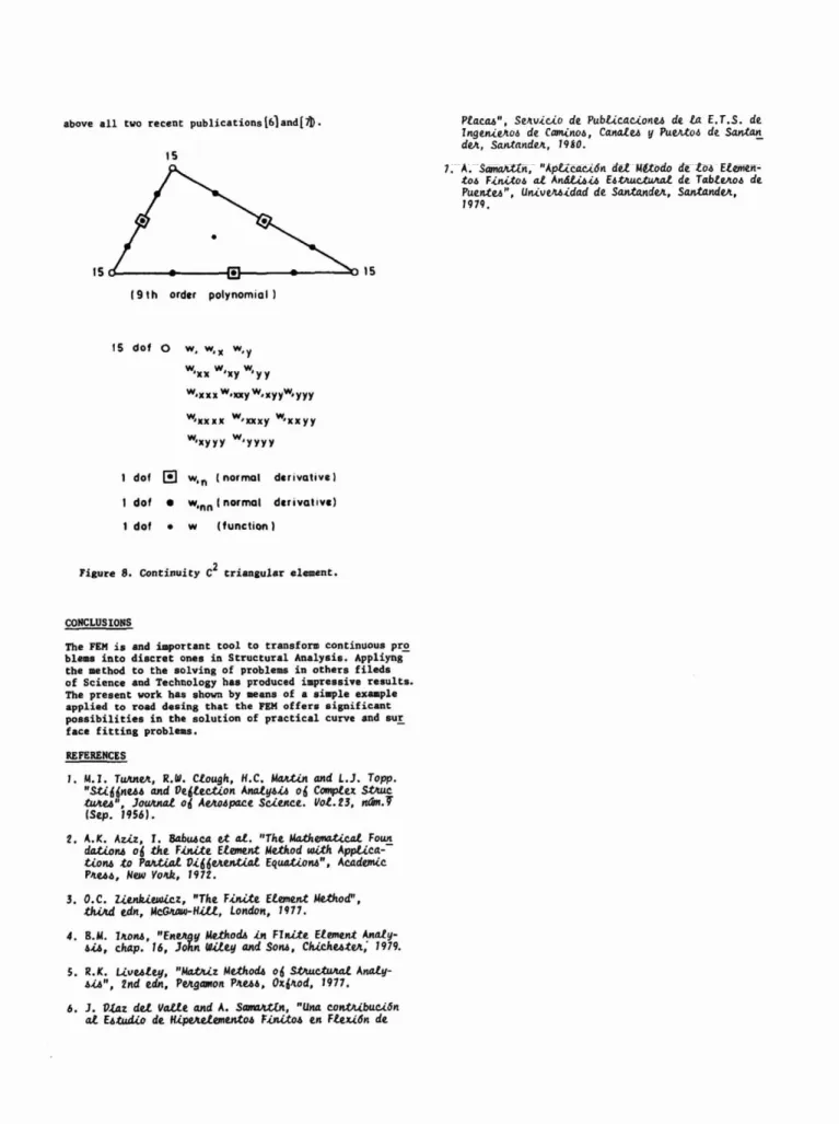
Finally, although the conexion with the planning of roads is less obvious, the method can be used succe ssfully along the lines indicated above for the re-presentation of surfaces (e.g. land rere-presentation), surfaces which passing through a series of points • pi(*i»yi»zi) *re found to be conditioned by simple

continuity requierements, including the fir9t deri vative or even the curvature. The most important aspect of the FEM both for this type of problem snd for other problems, involves the selection of shape or interpolation functions, since the comp£ sing and solving of the system of equations (11) is standard and can be found in any general matrix programmes of structures, for example: SAP, STRUDL, ANSYS, NASTRAN, etc. Figure B shows the possibili-ty of C2 element which might be used for this type of problem of smooth and continous surface repre-sentation. If only the continuity of the slope is required, the selection of triangular and compat_i ble elements is very wide, and these elements co-rrespond to all the compatible elements of bending of plates (refer to the specialised literature C A S E 6 7 8

I, 0 00 0 0 0 0 0 0

L2 33 33 6 6 6 6 3 3 3 3

Ls 6 6 67 9 0 00 9 0 0 0

Lt 133.33 1 1 0 0 0 110 0 0

L5 166 67 133 33 166 6 7

L6 2 0 0 00 200.00 200 00

above all two recent publications[6]and(^).

I S

Ptacat", SeAvi.CA.ci de PubUcacionu de la E.T.S. de Ingeiueloi de Caminot, Canalu y Pui/Uoi de Sanson deA, SantandeA, I960.

7. A. Soma/iitn, "kpU.aacu.6n del MfXodo de £04 Elemen-t s FiniElemen-toi aElemen-t An&LiElemen-tiElemen-t EiElemen-tAucluAaElemen-t de TabteAoi de PuenteV', UvuvtAtidad de SantandeA, SantandeA,

1979.

15 dof O w . w, x w.

w-xxx w-xxy w-xyyw<yyy

w'«xxx W' « x y w ,x x y y w ,« y y y w ,y y y y

1 dol s w ,n (normal derivative)

1 dot •

w ,n n 1 normal derivative) I dof • w (function 1

2

Figure 8. Continuity C triangular element.

CONCLUSIONS

The FEM is and important tool to transform continuous pro blems into discret ones in Structural Analysis. Appliyng the method to the solving of problems in others fileds of Science and Technology has produced impressive results. The present work has shown by means of a simple example applied to road desing that the FEM offers significant possibilities in the solution of practical curve and sur^ face fitting problems.

REFERENCES

1. M.I. TuAneA, K.IH. Clough, H.C. UcvuUn and L.J. Topp. "StCHntit and Perfection Analytit oi Complex StAuc tuA.it", JouAnat o\ AeAoipace Science. Vol. 13, ndn.7

(Sep. 1954).

2. A.K. Aziz, T. Babatca it at. "The. Mathematical Foun datlont oji the Finite Etement Method with Applica-tion* to PaAtlal t>HieAentlat Equationt", Academic Pieaa, New Yoik, 1172.

3. O.C. 2ie.nkituu.cz, "The Finite Element Method", thiAd edn, McGami-HM, London, 1177.

4. 8.M. lAont, "EneAgy Methods In finite Element Analy-tIt, chap. 16, John Wiley and Son4, ChlchesteAi 1979.

5. R.K. LiveAliy, "MatAlz Methodi oi StAuctuAal Analy-tic" , 2nd edn, PeAgamon Ptett, Ox(iod, 1977.