Biogeosciences, 6, 545–568, 2009 www.biogeosciences.net/6/545/2009/
© Author(s) 2009. This work is distributed under the Creative Commons Attribution 3.0 License.
Biogeosciences
Branch xylem density variations across the Amazon Basin
S. Pati ˜no1,2,*, J. Lloyd2, R. Paiva3,**, T. R. Baker2,*, C. A. Quesada2,3, L. M. Mercado4,*, J. Schmerler5,*,
M. Schwarz5,*, A. J. B. Santos6,†, A. Aguilar1, C. I.Czimczik7,*, J. Gallo8, V. Horna9,*, E. J. Hoyos10, E. M. Jimenez1, W. Palomino11, J. Peacock2, A. Pe ˜na-Cruz12, C. Sarmiento13, A. Sota5,*, J. D. Turriago8, B. Villanueva8, P. Vitzthum1, E. Alvarez14, L. Arroyo15, C. Baraloto13, D. Bonal13, J. Chave16, A. C. L. Costa17, R. Herrera*, N. Higuchi3,
T. Killeen18, E. Leal19, F. Luiz˜ao3, P. Meir20, A. Monteagudo11,12, D. Neil21, P. N ´u ˜nez-Vargas11, M. C. Pe ˜nuela1, N. Pitman22, N. Priante Filho23, A. Prieto24, S. N. Panfil25, A. Rudas26, R. Salom˜ao19, N.Silva27,28, M. Silveira29, S. Soares deAlmeida19, A. Torres-Lezama30, R. V´asquez-Mart´ınez11, I. Vieira19, Y. Malhi31, and O. L. Phillips2,*** 1Grupo de Ecolog´ıa de Ecosistemas Terrestres Tropicales, Universidad Nacional de Colombia, Sede Amazonia, Instituto
Amaz´onico de Investigaciones-Imani, km. 2, v´ıa Tarapac´a, Leticia, Amazonas, Colombia
2Earth and Biosphere Institute, School of Geography, University of Leeds, LS2 9JT, England, UK 3Institito National de Pesquisas Amazˆonicas, Manaus, Brazil
4Centre for Ecology and Hydrology, Wallingford, England, UK 5Fieldwork Assistance, Postfach 101022, 07710 Jena, Germany 6Departamento de Ecologia, Universidade de Bras´ılia, Brazil
7Department of Earth System Science, University of California, Irvine, USA 8Departamento de Biolog´ıa, Universidad Distrital, Bogot´a, Colombia
9Abteilung ¨Okologie und ¨Okosystemforschung, Albrecht-von-Haller-Institut f¨ur Pflanzenwissenschaften, Universit¨at
G¨ottingen, G¨ottingen, Germany
10Departamento de Ciencias Forestales, Universidad Nacional de Colombia, Medell´ın, Colombia 11Herbario Vargas, Universidad Nacional San Antonio Abad del Cusco, Cusco, Per´u
12Proyecto Flora del Per´u, Jard´ın Bot´anico de Missouri, Oxapampa, Per´u 13UMR-ECOFOG, INRA, 97310 Kourou, French Guiana
14Equipo de Gesti´on Ambiental, Interconexi´on El´ectrica S.A. ISA., Medell´ın, Colombia 15Museo Noel Kempff Mercado, Santa Cruz, Bolivia
16Lab. Evolution et Diversit´e’ Biologique CNRS, Univ. Paul Sabatier Bˆatiment 4R3, 31062, Toulouse cedex 4, France 17Universidade Federal de Par´a, Belem, Brazil
18Center for Applied Biodiversity Science, Conservation International, Washington, DC, USA 19Museu Paraense Emilio Goeldi, Belem, Brazil
20School of Geography, University of Edinburgh, Edinburgh, Scotland, UK 21Herbario Nacional del Ecuador, Quito, Ecuador
22Center for Tropical Conservation, Duke University, Durham, USA 23Universidade Federal do Mato Grosso, Cuiaba, Brazil
24Instituto de Investigaci´on de Recursos Biol´ogicos Alexander von Humboldt. Diagonal 27 No. 15-09, Bogot´a D.C, Colombia 25Department of Botany, University of Georgia, Athens, USA
26Instituto de Ciencias Naturales, Universidad Nacional de Colombia, Bogot´a, Colombia 27CIFOR, Tapajos, Brazil
28EMBRAPA Amazonia Oriental, Belem, Brazil
29Departamento de Ciˆencias da Natureza, Universidade Federal do Acre, Rio Branco, Brazil 30Facultad de Ciencias Forestales y Ambiental, Universidad de Los Andes, M´erida, Venezuela 31Oxford University, Centre for the Environment, Oxford, England, United Kingdom
†
deceased
*formerly at: Max-Planck-Institut f¨ur Biogeochemie, Jena, Germany
**now at: Secret´aria Municipal de Desenvolvimento e Meio Ammbiente ma Prefeturia Municipal de Mau´es, Mau´es, Brazil ***Authors are listed according to their contribution to the work.
546 S. Pati˜no et al.: Amazonian xylem density variation
Abstract. Xylem density is a physical property of wood
that varies between individuals, species and environments. It reflects the physiological strategies of trees that lead to growth, survival and reproduction. Measurements of branch xylem density, ρx, were made for 1653 trees represent-ing 598 species, sampled from 87 sites across the Amazon basin. Measured values ranged from 218 kg m−3for a Cordia
sagotii (Boraginaceae) from Mountagne de Tortue, French
Guiana to 1130 kg m−3for an Aiouea sp. (Lauraceae) from Caxiuana, Central Par´a, Brazil. Analysis of variance showed significant differences in averageρxacross regions and sam-pled plots as well as significant differences between families, genera and species. A partitioning of the total variance in the dataset showed that species identity (family, genera and species) accounted for 33% with environment (geographic location and plot) accounting for an additional 26%; the re-maining “residual” variance accounted for 41% of the total variance. Variations in plot means, were, however, not only accountable by differences in species composition because xylem density of the most widely distributed species in our dataset varied systematically from plot to plot. Thus, as well as having a genetic component, branch xylem density is a plastic trait that, for any given species, varies according to where the tree is growing in a predictable manner. Within the analysed taxa, exceptions to this general rule seem to be pio-neer species belonging for example to the Urticaceae whose branch xylem density is more constrained than most species sampled in this study. These patterns of variation of branch xylem density across Amazonia suggest a large functional diversity amongst Amazonian trees which is not well under-stood.
1 Introduction
Xylem tissue (wood) is a complex organic material com-posed of a matrix of hemicelluloses and lignin in which cellu-lose fibrils are embedded (Harada, 1965; Hamad, 2002; Pal-lardy and Kozlowski, 2007). It has a variety of functions in trees, such as structural support, actuation of the tree itself and of different organs (Niklas, 1992; Fratzl et al., 2008), long distance transport of water, inorganic ions, organic com-pounds and proteins from roots to leaves, and storage of wa-ter, carbohydrates and fat (Gartner, 1995; Smith and Shortle, 2001; Kehr et al., 2005). Wood also contains the major-ity of the carbon stored in a tree (Gartner, 1995). As the structure of xylem tissue changes as a result of environmen-tal requirements and phylogenetic constrains, so does xylem function (Carlquist, 1975; Tyree and Ewers, 1991; Niklas, 1992; Gartner, 1995; Tyree and Zimmermann, 2002; Bass et al., 2004) and the quantity of stored carbon within this tissue
Correspondence to: S. Pati˜no
too (Elias and Potvin, 2003). Density,ρ, (the ratio between oven-dry mass and fresh volume of xylem tissue) is one of the physical properties of wood (Kollmann and Cˆote, 1984) and provides an index of the balance between solid mate-rial (i.e. cell wall, parenchyma) and void (i.e. lumen of fi-bres, tracheids and conductive elements) of the xylem tissue. Therefore, changes in wood density are directly associated with structural variations at the molecular, cellular and organ levels. These structural differences are strongly correlated with the tree’s mechanical properties (Givnish, 1986; Niklas, 1992; Gartner, 1995), water transport efficiency and safety (Hacke et al., 2001; Tyree and Zimmermann, 2002; Jacob-sen et al., 2005; Holbrook and Zwieniecki, 2005; Pittermann et al., 2006), rates of carbon exchange (Tyree, 2003; Jacob-sen et al., 2005; Ishida et al., 2008) and perhaps resistance to pathogens and herbivores (Rowe and Speck, 2005). Different species from different taxonomic, phylogenetic and architec-tural groups show convergence of these functional character-istics in response to the environment (Meinzer, 2003).
In this work we make the distinction between the density of the wood from the main trunk (here defined as wood den-sity,ρw)normally measured at 1.3 m from the ground (pos-sibly including both sapwood and heartwood that may have been air or oven-dried) and that of the sapwood or functional xylem of small (ca. 1.5 cm diameter) terminal branches of trees (here defined as xylem density,ρx). Xylem density is considered as a potential proxy for tree hydraulic architecture (water transport) (Stratton et al., 2000; Gartner and Meinzer, 2005; Meinzer et al., 2008). There is evidence supporting the idea that hydraulic architecture may limit tree performance in terms of transpiration, carbon exchange and growth, (Tyree, 2003; Meinzer et al., 2008). For example, there have been reports showing how ρx scales negatively with leaf gas exchange and water balance for neotropical forest trees with contrasting phenologies subjected to contrasting rain-fall regimes (Santiago et al., 2004; Meinzer et al., 2008), for neotropical savannah trees (Bucci et al., 2004; Scholz et al., 2007), Hawaiian dry forests trees (Stratton et al., 2000) and Californian chaparral species (Pratt et al., 2007). For different environments (California chaparral, South African Mediterranean-type climate, Sonoran desert, Great Basin of central Utah) and for both gymnosperm and angiosperm trees and shrubs with distinct xylem structure (ring porous and dif-fuse porous),ρx scales positively with xylem resistance to cavitation and mechanical strength (Hacke et al., 2001; Pratt et al., 2007; Scholz et al., 2007; Jacobsen et al., 2007a, b; Dalla-Salda et al., 2008). It also, has been proposed that high density wood is necessary to avoid xylem implosion due to negative water tension inside xylem conduits (Hacke et al., 2001). These findings strongly suggest that xylem density could be used as a “trait” to predict the different physiologi-cal strategies of trees in tropiphysiologi-cal forests.
S. Pati˜no et al.: Amazonian xylem density variation 547 mechanical requirements (Asner and Goldstein, 1997;
Wag-ner et al., 1998; Taneda et al., 2004). Nonetheless, there are many important structural and functional differences be-tween branch and trunk wood as a result of different load-ing, hydraulic, architectural, and genetic constrains (Zobel and van Buijtenen, 1989; Gartner, 1995; Domec and Gart-ner, 2002; Cochard et al., 2005; Dalla-Salda et al., 2008). Trunk wood density may also be affected by factors in ad-dition to those modulatingρx. For example, it may reflect differences in the storage of resins or variation in the storage of secondary compounds within bole heartwood over time, or intrinsic species-specific differences on wood density gradi-ents within the main trunk (Wiemann and Williamson, 1988, 1989; Parolin, 2002; Knapic et al., 2008). In branches these additional effects may not occur, or at least not to the same extent.
It has long being known thatρwis a genetically conserved trait, and this characteristic has been used extensively in tree breeding (Zobel and van Buijtenen, 1989; Zobel and Jett, 1995; Yang et al., 2001). However, in plantations it is well known that for a given tree species, marked variations may also occur due to differences in genotype, climate, soil fac-tors and management (Cown et al., 1991; Beets et al., 2001; Roque, 2004; Thomas et al., 2005). In neotropical forests, particularly in the Amazon basin, site-specific differences have been noticed when comparing the same species grow-ing in different forests and/or site conditions (Wiemann and Williamson, 1989; Gonzalez and Fisher, 1998; Woodcock et al., 2000; Muller-Landau, 2004; Roque, 2004; Nogueira et al., 2005, 2007; Sch¨ongart et al., 2005; Wittmann et al., 2006). A special case of complex systems seems to be the Amazonian floodplains. When comparing the same species growing on nutrient-rich white water floodplains (v´arzea) and nutrient-poor black water floodplains (igap´o), Parolin (2002) and Parolin and Ferreira (2004) found higher ρw values in igap´o forest. Such differences might have been due to the combined effect of forest successional stages (young successional stages in the v´arzea and old-growth for-est in the igap´o) and differences in soil nutrient availabil-ity. For Macrolobium acciifolium studied in both habitats at the same successesional stage (old-growth forest) and at the same elevation showed that in v´arzea ρw was higher than in igap´o (Sch¨ongart et al., 2005). At the community level, lowρw is often associated with one or a combination of high soil fertility, high rates of forest disturbance, early and secondary successional vegetation and/or high rates of tree growth and mortality, (Saldarriaga, 1987; Wiemann and Williamson, 1989; Enquist et al., 1999; Woodcock et al., 2000; Roderick and Berry, 2001; ter Steege and Hammond, 2001; Muller-Landau, 2004; Baker et al., 2004b; Nogueira et al., 2005; King et al., 2005, 2006; Erskine et al., 2005; Wittmann et al., 2006; Chao et al., 2008; Slik et al., 2008).
The Amazon Basin is the most diverse and largest con-tiguous tropical forest on the planet (Malhi and Grace, 2000; Laurance et al., 2004). Different ecological systems and veg-etation formations with contrasting species compositions and life history traits (ter Steege et al., 2000, 2006), geological origins (Fittkau et al., 1975; Quesada et al., 2009a), climates (Sombroek, 2001; Malhi et al., 2004b), and an enormous diversity of soils (Sombroek, 2000; Quesada et al., 2009b) exist within its boundary creating a mosaic of forests and vegetation types with such a floristic complexity the basis of which is still not well understood (Phillips et al., 2003). How and why species are distributed (Leigh et al., 2004; Pitman et al., 2008), what explains differential productiv-ity (Malhi et al., 2004) and dynamic patterns across Amazo-nian regions (Phillips and Gentry, 1994; Phillips et al., 2002, 2004; Lewis et al., 2004; Baker et al., 2004a), how much car-bon is being absorbed and released to the atmosphere (Grace et al., 1995; Phillips et al., 1998; Malhi et al., 2000, 2004, 2006; Clark, 2002), how Amazonian forests are responding to global change (Phillips, 1997; Cox et al., 2000; Laurance et al., 2004; Wright, 2005; Phillips et al., 2009) are some of the questions that have motivated this research (Lloyd et al., 2009). By studyingρx across Amazonia we hoped to gain insights into the understanding of the functioning of Ama-zonian forests and, for the first time, rigorously examine the importance of both environmental and genetic controls on a plant trait over large scales for the tropical forest biome. By analysing the geographic and taxonomic patterns of branch xylem density from different trees and forests across Ama-zonia, we address the following three questions:
1. Are there detectable patterns ofρxacross Amazonia? If so, are those patterns related to taxonomic differences and/or to overall site conditions?
2. Are there differences in average values between forests and between different taxonomic groups?
3. Does the xylem density of particular species change across the basin according to the observed regional pat-terns?
548 S. Pati˜no et al.: Amazonian xylem density variation
2 Methods
2.1 Study sites
Eighty-seven forest plots from across the Amazon basin were sampled, typically at the end of the rainy season, between January 2001 and December 2005. Two plots were sampled in Paracou, French Guiana in September 2007 and seven ad-ditional plots were sampled between May 2007 and Septem-ber 2008 (see details below). The first 82 plots form part of the RAINFOR project (www.rainfor.org; Malhi et al., 2002) and span local, regional and Basin-wide environmental gra-dients. Many of the plots have been described in detail else-where (Vinceti, 2003; Malhi et al., 2004; Phillips et al., 2004; Baker et al., 2004a, b). The additional seven plots form part of the BRIDGE, ANR project (http://www.ecofog.gf/ Bridge/). Appendix A lists all the plots visited, including those not previously described, and in some cases with up-dated information.
2.2 Sampling of plant material
2.2.1 The RAINFOR protocol
Normally, around 20 trees greater than 10 cm dbh (diameter at breast height i.e. at 1.3 m from the base of the tree) were chosen in each plot for wood density sampling. On some oc-casions, such as when plots were unusually heterogeneous, as a consequence of topographic variations and/or shape (i.e. 1000×10 m) more trees were sampled (e.g. BOG-plots). For two of the Caxiuana plots (Central Par´a, Brazil) we sampled in two consecutive years (2002 and 2003) and since there was no statistical difference inρxfor the two years, we com-bined all this data for the following analyses. When a plot was clearly composed of different defined landscapes, and each landscape was considered as an individual plot, on aver-age 10 trees were sampled for each landscape (e.g. Jacaranda Plots, Km 34 Manaus, Brazil).
Trees were not chosen completely at random, sampling within each plot accounted for two factors. First, there was a selection of three to six contrasting areas (e.g. slopes, val-leys, gaps, creeks, swamps) where these were present. Sec-ondly, a professional tree climber then chose a “climbable tree” within the identified areas. Naturally, this “climbable tree” varied from climber to climber according to the tech-nique employed and overall climbing skills. Nevertheless a general consideration was that from the “climbable tree”, up-per branches (exposed to light) of at least three neighbouring trees were reachable, either by moving himself from tree to tree or by using a clipper pole. In each plot we also sam-pled branches from low, middle and upper crown from a sub-sample (three to 5 trees) of the total number of trees sub-sampled. These trees were selected on the basis of having three types of branches: upper canopy = exposed to light, middle = mid-light and lower = shaded.
2.2.2 The sampling strategy for the Guyaflux plots
For the Guyaflux plots, mostly lower branches from sub-canopy trees were sampled using a chain saw manipulated from the ground. To determine if data from lower branches introduces a bias in the data, we comparedρxof upper and lower branches from our sub-sample of 272 trees. We found no statistical differences between the density of branches from the two positions on the trees (ANOVA, DF=1, F=0.18,P=0.674, mean upper branches=619 kg m−3, mean lower branches=615 kg m−3). The ρx values of trees sam-pled at Paracou followed a normal distribution, and included the range of densities measured for ρw of 309 trees of a neighbouring plot. The composition of the trees sampled was also similar to the abundance distribution of the main families present in the Guyaflux plots (Jacques Beauchˆene, BRIDGE unpublished data).
2.2.3 The BRIDGE protocol
For the BRIDGE protocol, the sampling strategy was basi-cally the same: professional climbers selected “climbable trees” and from there moved across the canopy collecting upper branches from 70 to 100% of the trees present in the plots. From these branches 40 to 90% were used for xylem density determinations.
In order to assess the representativeness of the sampling strategy generally utilised across the Basin (usually only 20 trees per one hectare plot), we took advantage of the more comprehensive BRIDGE measurements to assess how repre-sentative this sampling strategy really was. Thus, for each comprehensively sampled BRIDGE plot we chose a sub-set of four clusters of five trees selected randomly across the sampled area (this also taking into account any topographic variability), comparing the estimated “plot level” values as calculated from these twenty trees only with the true plot mean.
2.3 Species identification
Details of the species identification from the permanent plots are described elsewhere (Baker et al., 2004b) and in this work we have used the new classification given by the Angiosperm Phylogeny Group II (APG 2003, http://www.mobot.org/ MOBOT/Research/APweb/), in which Bombacaceae,
Ster-culiaceae, and Tiliaceae are all included in the Malvaceae; Papilionaceae, Caesalpinaceae, and Mimosaceae are
in-cluded in the Fabaceae; Cecropiaceae in the Urticaceae; and
Flacourtiaceae in the Salicaceae.
2.4 Xylem density determinations
S. Pati˜no et al.: Amazonian xylem density variation 549
52 Figure 1
10°
0°
10°
50°
60°
70°
80°
80 – 76 75 – 71 70 – 66 65 – 61 60 – 56 55 – 51 50 – 46 45 – 41
7-SW-Venezuela 8-NE-Venezuela
5-Ecuador
6-Colombia 4-N-Peru
3-S-Peru & AC-Brazil
2-Bolivia
1-MT-Brazil
12-EP-Brazil
10-WP-Brazil 11-CP-Brazil 9-AM-Brazil
13-Guiana
Fig. 1. Spatial pattern of branch xylem density,ρx, for 87 forest
plots across the Amazon basin. Each symbol represents one plot. Symbol size represents the arithmetic meanρx (kg m−3).
Coor-dinates were changed to avoid overlapping points in the map and are listed in Appendix A. Numbers in blue indicate the respective Region for each plot. Abbreviations in regions follow those in leg-end for Appleg-endix A. Regions are : 1. MT-Brazil-; 2. Bolivia; 3. S-Peru and AC-Brazil-; 4. N-Peru; 5. Ecuador; 6. Colombia; 7. SE-Venezuela; 8. NE-Venezuela; 9. AM-Brazil; 10.WP-Brazil; 11. CP Brazil 12. EP -Brazil-EP, 13. F-Guiana.
within 12 h of sampling (but sometimes as long as 36 h later) the outer bark and phloem were removed from one of the two sample stems (the second sample was dried with the leaves and stored for possible further analysis) and its fresh volume calculated from its length and the average diameter of the two perpendicular diameters at each end. When the pith was wider than 2 mm diameter the stem was cut into a small seg-ment (0.02 to 0.05 m long) and the pith removed with a small screw driver or scalpel. When the pith was thinner than 2 mm it was not removed from the stem (as it was thus assumed to be of negligible mass) but its volume subtracted from the volume of the stem without bark. Pith volume was calculated by measuring the average diameter (two measurements of di-ameter at each end of the stem) and stem length. All stems were then dried at 70–90◦C for three to four days (to constant
mass) and weighed. Xylem density,ρx, was then determined as the dry mass divided by the green volume of the sample.
53 Figure 2
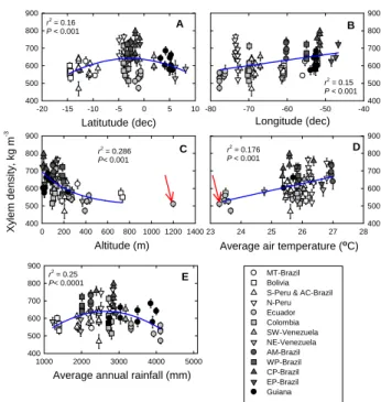
Altitude (m) 0 200 400 600 800 1000 1200 1400
X
y
lem densit
y
, kg m
-3
400 500 600 700 800 900
Average air temperature (oC)
23 24 25 26 27 28 400 500 600 700 800 900
Average annual rainfall (mm) 1000 2000 3000 4000 5000 400
500 600 700 800 900
r2 = 0.25
P< 0.0001
r2 = 0.286
P< 0.001 Latitutude (dec) -20 -15 -10 -5 0 5 10 400
500 600 700 800 900
Longitude (dec) -80 -70 -60 -50 -40
400 500 600 700 800 900
r2 = 0.16
P < 0.001
r2 = 0.15
P < 0.001
A B
C D
E MT-Brazil Bolivia S-Peru & AC-Brazil N-Peru Ecuador Colombia SW-Venezuela NE-Venezuela AM-Brazil WP-Brazil CP-Brazil EP-Brazil Guiana
r2 = 0.176
P < 0.001
Fig. 2. The relationship between branch xylem density for all 87
forest plots and (A) latitude; (B) longitude; (C) altitude; (D) mean annual temperature; and (E) total annual precipitation. Vertical lines are the standard error of means. Red arrow indicates a data point has been excluded from the analysis. Point corresponds to SUM-01, a premontane forest in Ecuador.
2.5 Statistical analysis
Basic statistics shown in Figs. 1, 3 and 4 were performed with Minitab 15 (Minitab Inc.).
In order to apportion the variance within the dataset (Searle et al., 2006) into geographical and taxonomic com-ponents, we fitted a model according to
ρx=µ+r/p+f/g/s+ε (1)
550 S. Pati˜no et al.: Amazonian xylem density variation
54 Figure 3
Xylem density, kg m-3
300 400 500 600 700 800 900 1000 300 400 500 600 700 800 900 1000
JAS-05 SUM-01 JAS-03 JAS-02 BOG-02 TIP-03 BOG-01 JAS-04 TIP-05 LSL-02 CHO-01 HCC-22 LFB-01 LSL-01 HCC-21 LFB-02 ELD-34 RIO-12 ELD-12 ALF-01 SIN-01 TAM-03 POR-01 DOI-02 POR-02 CUZ-03 TAM-01 RST-01 TAM-04 TAM-06 DOI-01 TAM-02 JUR-01 TAM-07 TAM-05 LOR-02 AGP-02 ZAR-02 AGP-01 LOR-01 ZAR-03 ZAR-04 ZAR-01 SCR-04 SCR-05 SCR-01 BAF-04 M17-11 NGL-11 GFX-07 ACA-11 TRE-01 NGH-20 GFX-09 SLV-01 TAP-04 TAP-01 TAP-03 TAP-02 YAN-02 YAN-01 SUC-01 ALP-12 SUC-04 JEN-11 SUC-02 ALP-11 ALP-22 SUC-03 ALP-21 JEN-12 ALP-30 MBO-01 CPP-01 BRA-01 MAN-02 MAN-04 MAN-01 MAN-05 MAN-03 BNT-04 CAX-02 CAX-01 CAX-05 JRI-01 CAX-03 CAX-04 N-Peru WP-Brazil SW-Venezuela
S-Peru & AC-Brazil
MT-Brazil NE-Venezuela Bolivia Colombia Ecuador Guiana CP-Brazil AM-Brazil EP-Brazil REGION
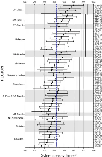
Fig. 3. Variation ofρx between and within regions. Regions and
plots are indicated in the left and right axes, respectively. Horizontal lines represent the standard deviation. Vertical straight lines repre-sent confidence limits defined using a Tukey test. Complementary information is given in Appendix B. Grey and white shadows sep-arate the regions. Vertical dashed-blue line represents the meanρx
of the basin.
All Standard Major Axis line-fittings for Fig. 6a, b, c were undertaken using SMATR package (Warton et al., 2006). Mixed-effect modelling (Fig. 7) was carried out using “lmne” (Bates and Sarkar, 2007) and rank-based linear regression (Fig. 8) accomplished as in Terpstra and McKean (2005), both using the “R” statistical computing package (R Devel-opment Core Team, 2007). For the latter analysis, we applied the “high-breakpoint” option to account for the possibility of “contaminated” data having been included in any of the ρwvalues assimilated from a wide range of sources into the RAINFOR “wood density” database.
In order to determine the extent to whichρx changed 1) in a given species within the same plot and between plots and 2) to estimate the variation within a given plot we cal-culated IPP (index of phenotypic plasticity) and IV (index of variation) respectively (Valladares et al., 2000). IPP and IV
were computed as the, absolute difference between the maxi-mum value and the minimaxi-mum value divided by the maximaxi-mum value.
3 Results
We measured ρx of 1653 trees (see supplementary material: http://www.biogeosciences.net/6/545/2009/ bg-6-545-2009-supplement.zip) from 87 plots (Appendix A) across the Amazon basin. Data for ρx followed normal distribution with mean and median values of 619 kg m−3 and 612 kg m−3, respectively; normality test (StDev=0.124, N=1653, AD=1.202P <0.005).
Of all the trees sampled, 95% (1568) had been identi-fied to the family level, 89% (1475) to the genus level, and 72% (1199) to the species level. The trees sampled ac-counted for 60 families, representing 41% of the total num-ber of families present in the neotropics (Mass and Wes-tra, 1993) with 283 genera, and 598 species being sam-pled. The most common families sampled in our data set in order of abundance were Fabaceae, Sapotaceae,
Lecythi-daceae, Moraceae, Burseraceae, Myristicaceae, Lauraceae, Annonaceae, Euphorbiaceae, Chrysobalanaceae, with the
most common genera being Eschweilera, Pouteria, Protium,
Inga, Licania, Virola, Pseudolmedia, Pourouma, Lecythis, Miconia. The most common species were Eschweilera co-riacea, Pseudolmedia laevis, Rinorea guianensis, Tetragas-tris altissima, Minquartia guianensis, Pourouma guianen-sis, Pseudolmedia macrophylla, Lecythis persistens, Miconia poeppigii, and Pourouma minor. At the family level we had
86 (5%) undetermined individuals. At the genus level we had 21 undetermined Protium sp., 18 Pouteria sp., 14 Inga sp., 11 Ocotea sp., 11 Eschweilera sp., 10 Virola sp. among others. The distribution of families and genera in our dataset represents well previous descriptions of floristic composition across Amazonia (Terborgh and Andresen, 1998; ter Steege et al., 2000, 2006).
3.1 Geographic variation
Arithmetic means ofρxfor the 87 plots are shown in Fig. 1, which also shows our separation into 13 discrete geograph-ical regions mainly determined by the proximity of plots. These regions are used for subsequent analysis.
S. Pati˜no et al.: Amazonian xylem density variation 551 55 Figure 4 OLA CEL CHR HUM OCH LIN RHI SCR APO MYRT LEC SIM SAPO AQUI STYR SAPI FAB CLU CAR VIO VER RUB NYC ANA RUT MELA ICA SAL COM LAU ROS MELI ULM BUR
GENUS FAMILY GENUS FAMILY GENUS FAMILY
PRO MALP OLEA MON POL MOR EUP BIG DIC ARAL VOC URT MYRI ANN MALV STA RHA LAC LEP SAB BIX BOR IXO MYRS ELA *
Dx, kg m-3
300 600 900 1200
Emmotum Poraqueiba Dendrobangia Metteniusa Buchenavia Terminalia Dasynema Sloanea Anthodiscus Mouriri Miconia Rinorea Rinoreocarpus Amphirrhox Leonia Paypayrola Stachyarrhena Botryarrhena Guettarda Duroia Calycophyllum Pentagonia Simira Amaioua Ixora Coussarea Ferdinandusa Chimarrhis Palicourea Capirona Posoqueria Alseis Vitex Metrodorea Galipea Zanthoxylum Neea Peridiscus Laetia Casearia Hasseltia Lunania Banara Aiouea Licaria Mezilaurus Pleurothyrium Sextonia Nectandra Ocotea Anaueria Caryodaphnopsis Rhodostemonodaphne Aniba Chlorocardium Cryptocarya Endlicheria Cinnamomum Simaba Picramnia Simarouba Trichilia Swietenia Carapa Guarea Cedrela Cabralea Prunus Celtis Tapirira Thyrsodium Euplassa Crepidospermum Protium Dacryodes Tetragastris Chionanthus Bunchosia Byrsonima Siparuna Coccoloba Triplaris
Dx, kg m-3
300 600 900 1200
Cyrillopsis Schoepfia Minquartia Aptandra Heisteria Chaunochiton Licania Couepia Hirtella Parinari Maytenus Goupia Sacoglottis Vantanea Ouratea Roucheria Hebepetalum Bontia Rhizophora Cassipourea Sterigmapetalum Haploclathra Tovomita Garcinia Clusia Symphonia Caraipa Calophyllum Chrysochlamys Myrcia Eugenia Aspidosperma Malouetia Geissospermum Mucoa Ambelania Anartia Himatanthus Laxoplumeria Collophora Macoubea Corythophora Gustavia Bertholletia Eschweilera Lecythis Couratari Grias Melicoccus Talisia Cupania Vouarana Matayba indet Prieurella Diploon Manilkara Pouteria Chrysophyllum Pradosia Ecclinusa Lucuma Micropholis Ilex Styrax Vatairea Dipteryx Machaerium Bocoa Newtonia Crudia Campsiandra Cedrelinga Vouacapoua Hymenolobium Lonchocarpus Brownea Andira Taralea Cynometra Swartzia Copaifera Diplotropis Pterocarpus Poecilanthe Toluifera Naucleopsis Pithecellobium Tachigali Hymenaea Sclerolobium Dialium Parkia Enterolobium Pseudopiptadenia Macrolobium Peltogyne Abarema Inga Batesia Clathrotropis Aldina Ormosia Eperua Mora Bauhinia Dicorynia Erythrina Amerimnon Piptadenia Albizia
Dx, kg m-3
300 600 900 1200
Sandwithia Sagotia Hieronyma Senefeldera Micrandra Drypetes Pau Maprounea Mabea Nealchornea Hevea Tapura Caryodendron Sapium Phyllanthus Glycydendron Margaritaria Amanoa Conceveiba Pera Croton Alchornea Hyeronima Tetrorchidium Naucleopsis Sahagunia Trymatococcus Sorocea Clarisia Perebea Maquira Pseudolmedia Trophis Brosimum Olmedia Ficus Helicostylis Castilla Bagassa Poulsenia Tabebuia Jacaranda Oxandra Ephedranthus Duguetia Tetrameranthus Bocageopsis Pseudoxandra Guatteria Unonopsis Xylopia Rollinia Porcelia Onychopetalum Annona Schefflera Dendropanax Coussapoa Pourouma Qualea Vochysia Erisma Iryanthera Virola Osteophloeum Otoba Huertea Turpinia Rhamnidium Catostemma Pachira Scleronema Ceiba Sterculia Theobroma Quararibea Apeiba Matisia Lueheopsis Luehea Lacistema Ruptiliocarpon Meliosma Bixa Cerdana Cordia
Fig. 4. Variation of xylem wood density,ρx(kg m−3), between and within families. Each dot represents the averageρxof each genus. Left
vertical axes represent genera, right vertical axes represent families and X-axis is theρx. Grey and white shadows separate the families.
Vertical dashed-blue line represents the meanρxof the basin. Horizontal lines represent the Standard Deviation. Families in the Figure
are sorted from high to lowρx from top-right (A) to left-bottom (C). The three panels (A, B, and C) represent one continuous Figure,
divided only for purpose of presentation. Abbreviation of the families are listed below ρx: IXO=Ixonanthaceae, OLA=Olacaceae,
CHR=Chrysobalanaceae, CEL=Celastraceae, HUM=Humiriaceae, OCH=Ochnaceae, LIN=Linaceae, SCR=Scrophulariaceae,
RHI=Rhizophoraceae, CLU=Clusiaceae, MYRT=Myrtaceae, APO=Apocynaceae, LEC=Lecythidaceae, SAPI=Sapindaceae,
MYRS=Myrsinaceae, SAPO=Sapotaceae, AQUI=Aquifoliaceae, STYR=Styracaceae, FAB=Fabaceae, ICA=Icacinaceae,
COM=Combretaceae, ELA=Elaeocarpaceae, CAR=Caryocaraceae, MELA=Melastomataceae, VIO=Violaceae, RUB=Rubiaceae,
VER=Verbenaceae, RUT=Rutaceae, NYC=Nyctaginaceae, SAL=Salicaceae, LAU=Lauraceae, SIM=Simaroubaceae, MELI=Meliaceae, ROS=Rosaceae, ULM=Ulmaceae, ANA=Anacardiaceae, PRO=Proteaceae, BUR=Burseraceae, OLEA=Oleaceae, MALP=Malpighiaceae,
MON=Monimiaceae, POL=Polygonaceae, EUP=Euphorbiaceae, DIC=Dichapetalaceae, MOR=Moraceae, BIG=Bignoniaceae,
ANN=Annonaceae, ARAL=Araliaceae, URT=Urticaceae, VOC=Vochysiaceae, MYRI=Myristicaceae, STA=Staphyleaceae,
RHA=Rhamnaceae, MAL=Malvaceae, LAC=Lacistemataceae, LEP=Lepidobotryaceae, SAB=Sabiaceae, BIX=Bixaceae, and
552 S. Pati˜no et al.: Amazonian xylem density variation tended to have lower ρx compared to regions paralleling
Amazon River (some plots in N-Peru and Colombia, AM-Brazil, WP-AM-Brazil, CP-AM-Brazil, EP-Brazil). To explore this trend, plot coordinates (latitude and longitude), altitude, mean annual temperature, and mean annual rainfall (see Ap-pendix A) were plotted against xylem density (Fig. 2). High density sites were located between 0◦ and−5◦ while low density sites occurred in all the latitudinal range covered by this study: ≈10◦ to −15◦ (Fig. 2a). Xylem density also tended to increase from West to East (Fig. 2b) as has been reported forρw(Baker et al., 2004b; Chave et al., 2006; ter Steege et al., 2006). The western margin is marked by the lowρx of the Ecuadorian plots (Fig. 2b). These were the plots closest to the Andes with higher altitudes (Fig. 2c), lower annual mean temperatures (Fig. 2d), higher annual rainfall (Fig. 2e), and more fertile soils (Malhi et al., 2004; Quesada et al., 2008). The Eastern most plots, located in EP-Brazil include a mangrove forest which had higherρxthan rest of forest plots in the same region (Region 12, Fig. 1). An inverse relationship between altitude andρx (Fig. 2c) and a positive relationship with average air temperature (Fig. 2d) points to an effect of environmental conditions uponρx. Low density sites are found in the two extremes of the rainfall range (Fig. 2e). In the low rainfall range (Bolivia and NE-Venezuela for example) there are the Bolivian seasonally flooded (LSL-01 and LSL-02), liana (CHO-01) and gallery forests plots (HCC-21 and HCC-22) where soils may retain enough soil moisture thus high soil water potential during the dry season. In the rest of the Bolivian and Venezue-lan forests, trees may have distinct mechanisms common in seasonal forests such as low density wood, high stem water storage capacity and/or deciduous leaves (Choat et al., 2005) to cope with prolonged drought. In the high rainfall range there are the low density Ecuadorian sites and the intermedi-ate density Guiana plots.
Taking the Basin as a whole (no division into regions), sta-tistically significant differences existed between plot means (P <0.001) ranging from 800±50 kg m−3(±standard devi-ation) at the dry experimental plot at Caxiuana (Projecto Se-caflor), CAX-04, with the nearby control plot CAX-03 be-ing the second highest at 780±120 kg m−3. These are both
terra firme forests on acrisol soils with 80% sand in its upper
layer (Quesada et al., 2009b). The lowest plot means were for TAM-03, a swamp forests in Tambopata, and JAS-05 a forest growing on recently deposited river sediments (fluvi-sol) in Jatun Sacha in Ecuador. Both these plots had a mean ρx of 470 kg m−3. Data for all 87 plots are summarised in Appendix B.
Figure 3 gives means (±standard deviations) for all plots, grouped according to region, with regions being presented sequentially from top to bottom according to the overall meanρxfor the trees sampled within them. This shows that, although considerable plot-to-plot variation existed within regions (e.g. N-Per´u and Colombia) large statistical differ-ences between regions also existed (P <0.001). Of these, the
highest overall value was for CP-Brazil (754±126 kg m−3, N=143) which had significantly higherρx(Tukey Test) than the rest of the regions while Ecuador had the lowest over-all values (535±89 kg m−3). Nevertheless, Ecuador did not differ significantly from Bolivia, S-Per´u and AC-Brazil, MT-Brazil, and Colombia. Within some regions: PC-MT-Brazil, PE-Brazil, N-Per´u, PW-PE-Brazil, Colombia, S-Per´u, MT-Brazil and Ecuador, mean ρx of plots varied considerably (Ap-pendix B), while in some regions Bolivia, AC-Brazil, NE-Venezuela, SW-NE-Venezuela, plots were not significantly dif-ferent from each other. The most variable plots were TAP-04, CAX-02, M17-11 (IV=0.76, 0.76 and 0.73, respectively) with the least variable being BNT-04, YAN-02, ALP-12 and TAP-03 (IV=0.24, 0.27, 0.27, and 0.27, respectively). IV values for all the plots can be seen in Appendix B.
3.2 Taxonomic variation
In a similar manner to the Region/Plot analysis above, variation in ρx at the family and genera level is sum-marised in Fig. 4. Overall there were significant dif-ferences between the families sampled (F=8.08 DF=57 P <0.001). Families with ρx higher than the basin mean were Olacaceae, Celastraceae, Chrysobalanaceae,
Humiri-aceae, OchnHumiri-aceae, LinHumiri-aceae, ScrophulariHumiri-aceae, MyrtHumiri-aceae,
and Lecythidaceae. Families with lower ρx were
Boragi-naceae, Bixaceae, Sabiaceae, Lepidobotryaceae, Lacistem-ataceae, Rhamnaceae, Malvaceae, Annonaceae, Myristi-caceae, UrtiMyristi-caceae, Vochysiaceae, Araliaceae,
Dichapeta-laceae, Bignoniaceae, and Euphorbiaceae. The
remain-ing families all contained genera characterised by both high and low ρx and include some of the most abun-dant families across the basin: Fabaceae, Rubiaceae,
Lauraceae, Sapotaceae, Apocynaceae (Fig. 4). There
were also significant differences between genera (F=3.78
DF=249 P <0.0001) with the highest density genera
be-ing Aiouea, Callichlamys, Pithecellobium, Vatairea,
Stach-yarrhena, Dipteryx, and Machaerium. The genera with the
lowest densities were Annona, Matisia, Tetrorchidium,
Col-lophora, Onychopetalum, Hyeronima, and Luehea.
3.3 Partialling out geographical and taxonomic
differ-ences
S. Pati˜no et al.: Amazonian xylem density variation 553
56
Figure5
Region 20%
Plot 6%
Family 14%
Genus 9% Species
10% Residual
41%
Fig. 5. Apportion of the total variance ofρxin the data set. The
analysis includes only fully identified species (1198 individuals).
of architectural changes due to space constraints (Cochard et al., 2005), but also incorporating any measurement error. The analysis here differs from others (Baker et al., 2004b; ter Steege et al., 2006; Chave et al., 2006) in that we have not taken overall means for each species, but rather included intra-specific variation and the possibility of systematic plot-to-plot variations in our interpretation. Figure 5 thus suggests that geographic location is as important as taxonomic iden-tity in determining the value ofρx observed for any given tree but with considerable variation accountable for by nei-ther. The first point is demonstrated further in Fig. 6, where we have taken the more widely abundant families (Fig. 6a) genera (Fig. 6b) and species (Fig. 6c) in our data set and plot-ted the average values observed in each of the plots were they were sampled as a function of the average density of all other trees sampled in the same plot. Our hypothesis had been that ρxof the most abundant families, genera and species across the basin would scale isometrically with the average of all other trees in the plot where they were found and thus we ra-tionalised thatρxof individuals of the same species growing in different forests will reflect the mean values of the other trees in the same plot. Thus, we tested for a common slope amongst all the groups containing more than four observa-tions at each taxonomic level. We found significant statisti-cal indications that at the three levels there where common slopes, but in all cases the slopes fitted were significantly greater than 1.0: for families the common slope was 1.45, for genera 1.40 and for species 1.28 (Appendix C). We further tested for differences in elevation and shift across the SMA common slope and at the three levels there were significant shifts in elevation and along the common slopes. Notable exceptions did however exist for the Urticaceae (Fig. 6a,
57
Figure 6A
300 450 600 750 900 300 450 600 750 900
Mean of Family
in plot (
X
y
lem dens
ity
,
kg
m
-3)
300 450 600 750 900
300 450 600 750 900
300 450 600 750 900
300 600 900 300 600 900
Mean of plot without Family (Xylem density, kg m-3) 300 600 900
300 600 900 300
450 600 750 900
Burseraceae
Chrysobalanaceae
Moraceae
Lauraceae
Fabaceae Lecythidaceae
Euphorbiaceae Malvaceae
Urticaceae
Myristicaceae Annonaceae
Meliaceae
Rubiaceae
Olacaceae Sapotaceae
Violaceae Apocynaceae
Clusiaceae Melastomataceae
A B C
E
D
F G
I
H
J K L
O N
M P
Q R S T
U V W X
Vochysiaceae
Icacinaceae Sapindaceae
Elaeocarpaceae Bignoniaceae
Fig. 6a. Pairwise relationships between meanρx of plot (X-axis)
and meanρxof each family (A), genera (B), and species (C) within
each plot. For each fitted line a plot mean was calculated excluding the family, genera or species for which the analysis was done and plotted against the average of that family, genus or species. Families used in the analysis were collected in at least 6 plots; genera in at least 8 plots and species in at least 6 plots. Regression lines in blue where not highly significant although follow the general trend. No regression lines in panels (A) M and U; (B) G and I; and (C) F, K, and M indicate that there were not significant relationships. All analysis were performed using SMATR.
panel T), that consist mostly of pioneer species (Whitmore, 1989). Non-significant relationships might be related to the “pioneer” character of the examined species i.e. Pourouma
minor, Pourouma guianensis and also related to the reduced
number of observations. Detailed outputs of all the analyses are given in Appendix C.
3.4 Geographical and taxonomic contributions to stand
level differences
554 S. Pati˜no et al.: Amazonian xylem density variation
58 Figure 6B
Mean of Genus
i n pl ot (Xy lem dens it y , k g m -3) 300 450 600 750 900 300 450 600 750 900 300 450 600 750 900
300 600 900 300 600 900
Mean of plot without Genus (Xylem density, kg m-3) 300 600 900
300 600 900 300 450 600 750 900 Licania Miconia Inga Pseudolmedia Eschweilera Protium Lecythis Tachigali Ocotea Virola Pourouma Aspidosperma Rinorea Pouteria Micropholis Brosimum
A B C
E
D
F G
I
H
J K L
O N
M P
Q R S T
U V W X
Guarea Swartzia Minquartia Duguetia Drypetes Manilkara Sloanea Unonopsis 300 450 600 750 900 300 450 600 750 900
Fig. 6b. Continued.
effects, we utilised estimates of the individual plot and species effects from Eq. (1) and compared them to direct stand-level calculations. This was achieved by first estimat-ing the average value for each species within each plot and then obtaining a weighted average value forρxfor that plot according to the observed abundance of each species within it, denoted here ashρxi. A similar calculation was done for the REML “species effects” which are plotted along with REML fixed plot effects (ther/pterm from Eq. 1) as a func-tion ofhρxi in Fig. 7. This analysis shows that by far the most of the variation inhρxi was accountable in terms of plot-to-plot differences, with the plot effects increasing al-most linearly withhρxiwith a slope close to 1.0. By contrast the species (i.e.f/g/s)effects were more or less constant (and close to zero) forhρxi>ca. 550 kg m−3, although de-clining slightly thereafter. We treated our plot term as a fixed effect for the analysis in Fig. 7 (as opposed to a random effect in Fig. 5), as this permitted us to allow for different plots to have different intrinsic variances consistent with differences in topography and soils heterogeneity between the various plots. This also removed a slight bias in the residuals which was present when treating ther/pterm as random.
59 Figure 6C 300 450 600 750 900 300 450 600 750 900 M e an o f s p e c ie s in pl ot (X y le m de ns it y , k g m -3) 300 450 600 750 900 300 450 600 750 900
300 600 900 300 600 900
Mean of plot without species (Xylem density, kg m-3) 300 600 900
300 600 900 300 450 600 750 900 Pseudol.macrophylla
Eschweilera coriacea Lecythis idatimon Pouteria cuspidata
Pseudolmedia laevis Protium decandrum
Virola calophylla Virola pavonis Micropholis guyanensis
Iryanthera juruensis
Tetragastris panamensis
Micrandra sprucei
Otoba glycycarpa
A B C
E
D
F G
I
H
J K L
O N
M P
Q R S T
Scleronema micranthum Pourouma minor Licania heteromorpha
Pourouma guianensis Rinorea guyanensis Minquartia guianensis Laetia procera
Fig. 6c. Continued
3.5 Phenotypic plasticity and index of variation
In order to determine the intra-specific variation we com-pared the IPP of the same species collected several times within one plot and over several plots. The IPP of individual species collected in more than two plots (mean=0.29±0.13, N=19) was significantly higher (mean=0.15±0.07, N=86) than the variation of the same species collected more than twice within one plot (DF=1,F=16.24,P <0001). IPP val-ues are given in Appendix D.
4 Discussion
Our results show that there are significant variations of branch xylem density across Amazonia with regional and local patterns and with considerable plasticity observed for many species growing in different forests. This suggests that branch xylem density may not be a simple genetically inher-ited trait that is predictable on the basis of the knowledge of plant taxonomy alone, and that across the Basin patterns of branch xylem density may not be only explained by patterns of species composition and abundance as has previously been considered to be the case forρw(Baker et al., 2004b; Chave et al., 2006; ter Steege, 2006).
S. Pati˜no et al.: Amazonian xylem density variation 555
60
Figure 7
Plot level (abundance weighted) Dx , kg m-3
400 450 500 550 600 650 700 750 800
REML e
ffec
t, kg
m
-3
-150 -100 -50 0 50 100 150
Species Plot
Fig. 7. The contribution of estimated plot effects (ther/pterm of Eq. (1) and estimated genotypic effects (thef/g/sterm of Eq. (1) to stand level variations in wood density.
2006). Local differences may be associated to topographic and physiognomic variations along with soil chemical and physical properties. In plantations it is well known that the addition of nutrients (e.g. N and/orP) reduces wood den-sity (Beets et al., 2001; Wang and Aitken, 2001; Thomas et al., 2005) and plots paralleling the Andes generally have higher soilP availability than those paralleling the Amazon River (Quesada et al., 2009b). Patterns ofρx across Ama-zonia support the idea that species are not randomly dis-tributed across landscapes but follow the “habitat tracking” hypothesis (Ackerly, 2003). For example, irrespective of the taxonomic level examined (Fig. 6), ρx observed varied by as much as 400 kg m−3 across sites. Moreover, this vari-ation was systematic with different trees sampled within a given family/genus/species tending to have higher values of ρxalong with other trees in the same plot (and vice versa). At each taxonomic level there was a common slope which was steeper than one, indicating that, at least for the widespread species examined in this study there exists considerable phe-notypic plasticity inρx; i.e. there is long term acclimation and thus adaptation of the xylem tissue to any given envi-ronment. That the slopes in Fig. 6 fitted through SMA are consistently greater than 1.0, suggests a continual replace-ment of species towards the maximum end of theirρxrange by species with a characteristically lowerρxunder the same growth conditions. Additional evidence for widespread plas-ticity comes from the REML variance partitioning of Fig. 5 in which the combined effects of Region/Plot are shown to have contributed to about the same proportion of the overall variation in the data set as did Family/Genus/Species.
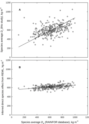
Since wood density is an important parameter in esti-mating forest carbon stocks (Baker, 2004a) one question to answer was: can ρw be predicted by knowledge ofρx? We examined our species level means forρx as a function
61 Figure 8
Specie
s a
v
e
rage
Dx
(t
h
is
st
u
d
y
),
k
g
m
-3
0 200 400 600 800 1000 1200
Species average Dw (RAINFOR database), kg m-3
0 200 400 600 800 1000 1200
Inferred direc
t s
p
ec
ies
effec
t
from
REML,
kg m
-3
0 200 400 600 800 1000 1200
A
B
Fig. 8. The relationship between (A) observed species level values
for xylem density (ρx)obtained in the current study and species
level mean values for wood densityρw obtained from the
RAIN-FOIR database and (B) deduced species level effects onρxfrom the
REML analysis of Eq. (1) and mean values ofρwfrom the
RAIN-FOR database.
of species mean ρw using an expanded database (RAIN-FOR wood density data base) from that presented in Baker et al. (2004b). We found a reasonably good relationship (Fig. 8a). Similar results have been shown for Puerto Rican (Swenson and Enquist, 2008), Colombian (Juliana Agudelo and Pablo Stevenson, unpublished data) and Guiana forest species (Sarmiento et al., 2008). It is worth noting that the average ρx for this study i.e. for the Amazon basin, (619 kg m−3) is very similar to previous values reported for
ρw for Amazonia. For example, Brown et al. (1984) esti-mated 620 kg m−3 as the average wood density of tropical America, Chave et al. (2006) reported 650 kg m−3for Cen-tral and South America together and (Baker et al., 2004b) estimated 620 kg m−3 as the overall species-level mean for Amazonia.
556 S. Pati˜no et al.: Amazonian xylem density variation and genetic variations. There is a strong tendency of many
species, genera and even families to be geographically con-fined to certain areas of the Basin (ter Steege et al., 2006) and thus, if there is some equivalence betweenρx andρw, what has previously been interpreted as a solely genetic ef-fect for the latter, may in fact be partly a geographic (site and regional) effect: this being attribute to variations in climate, and soils. In that respect it is only by studying replicated species growing across a wide range of environments that we have been able to show the strong environmental influ-ence onρx(and by implicationρw). For example we show that altitude is negatively correlated withρx(Fig. 2c) and this effect has been suggested forρw(Wiemann and Williamson, 1989; Chave et al., 2006). Temperature was also positively correlated withρx as shown in Fig. 2d. The physical basis of this effect of temperature on wood density (water viscos-ity decreases as temperature increases) has been proposed by Roderick and Berry (2001) and has been experimentally sup-ported by Thomas et al. (2004). There is also evidence that physical and chemical properties of soils may have an influ-enceρw(Hacke et al., 2000; Parolin, 2004; Parolin and Fer-reira, 2004). In essence the REML species effect in Fig. 8b forρxrepresents the inferred value that each species would have were it to be found on some sort of “overall average site”.
It is also worth noting that, in contrast to the general trend, long-lived pioneer species (Whitmore, 1989) within the
Ur-ticaceae often associated to gap colonisation, secondary
veg-etation and/or late stages of forest succession, showed little tendency to exhibit variation inρxacross the sites where they were found (Fig. 6a, panel T, respectively). This brings the question of whether species showing little phenotypic plas-ticity and intermediateρx values are present in sites where the majority of trees have relative low xylem density. These species when found in terra firme old grow forests (this study) may be more restricted to specific edaphic and micro-climatic conditions that sustain colonisation and fast growth (i.e. gaps with enough water supply from the soil, nutrients, optimal temperature, not too much wind, sufficient light). This is because if they where in a high density site (stressful conditions) they could not cope with the environment. Also, species such as Pourouma minor and P. guianensis, which are generally considered low-density, fast-growing species did not have the lowest branch densities in our study; xylem density varied from 410 to 690 kg m−3; comparable to some of the slow-growth climax species observed.
Further evidence of the influence of site conditions on ρx of trees comes from our own data. In a Mangrove for-est in East Par´a, Brazil (EP-Brazil, BRA-01, Appendix A) only two species were sampled (10 individuals per species)
Avicennia germinans and Rhizophora mangle which mean
ρx were 722±87 kg m−3and 723±99 kg m−3, respectively. The two species are not phylogenetically related since they belong to two different families (Scrophulariaceae and
Rhizophoraceae) and two different orders (Lamiales and
Malpighiales). Nevertheless they converged to an almost
identical highρx. Mangroves are well known for having spe-cial water dynamics, fluctuating salinity, low oxygen concen-tration in the soil, and particular soil chemical and physical characteristics (Lovelock et al., 2006a). These environmen-tal factors constrain tree water relations, gas exchange and growth (Lovelock et al., 2006b).
As suggested from experimental studies done on different species from different environments, highρx is an adaptive response to severe environmental conditions such as drought (Dalla-Salda et al., 2008), high temperature (Thomas et al., 2004), porous soils (Hacke et al., 2000), poor nutrient con-ditions and long periods of high floods (Beets et al., 2001; Wang and Aitken, 2001; Thomas et al., 2005; Wittmann et al., 2006). For Amazonian species it is difficult to imagine that highρx, of the order we have found (for example from 750 kg m−3to 1130 kg m−3)are directly associated with
ex-treme drought conditions – those regions of the Amazon where severe water stress is most likely to occur are those re-gions with a long dry season i.e. Bolivia, parts of Venezuela, Guiana, and East Brazil. These regions were characterised by low and intermediateρx. High xylem density most likely is related to variation in resource availability and/or differ-ent site dependdiffer-ent soil physical characteristics and hydro-logical constraints. ρx is a trait that reflects environmen-tal constrains (Cochard et al., 2008), and so aggregation of species according to ρx (ter Steege et al., 2006, for exam-ple) should also reflect environmental constraints imposed upon “species” of trees. We conclude that variations ofρx across basin reflect an enormous functional diversity among trees and Amazonian forests. Any change inρxmay reflect changes at various levels of organisation. For example, as ρx increases, microfibril angle, cell wall thickness, modu-lus of elasticity and resistance to cavitation also increase, but hydraulic efficiency and rates of gas exchange decrease. Ad-ditional studies on these subjects, particularly how variations inρxrelates to other plant physiological characteristics (e.g. Fyllas et al., 2009) are needed to better understand the func-tional diversity of Amazonian trees.
Appendix A
S. Pati˜no et al.: Amazonian xylem density variation 557
Table A1.
Plot Name and Description Region Code Region Plot Code latitude longitude Altitude (m) MeanT(◦C) Forest Type Principal Investigator
Sinop 1 MT-Brazil SIN-01 −11.41 −55.33 325 25.4 Terra firme M. Silveira
Alta Foresta 1 MT-Brazil ALF-01 −9.60 −55.94 255 25.6 Terra firme M. Silveira
Los Fierros Bosque I 2 Bolivia LFB-01 −14.56 −60.93 230 25.1 Terra firme T. Killeen
Los Fierros Bosque II 2 Bolivia LFB-02 −14.58 −60.83 225 25.1 Terra firme T. Killeen
Huanchaca Dos, plot1 2 Bolivia HCC-21 −14.56 −60.75 720 25.1 Gallery L. Arroyo
Huanchaca Dos, plot2 2 Bolivia HCC-22 −14.57 −60.75 735 25.1 Gallery L. Arroyo
Las Londras, plot 1 2 Bolivia LSL-01 −14.41 −61.14 170 25.9 Seasonally flooded L. Arroyo
Las Londras, plot 2 2 Bolivia LSL-02 −14.41 −61.14 170 25.9 Seasonally flooded L. Arroyo
Chore 1 2 Bolivia CHO-01 −14.39 −61.15 170 25.9 Liana forest T. Killeen
Tambopata plot zero 3 S-Peru TAM-01 −12.84 −69.29 205 25.1 Terra firme O. Phillips and R. Vasquez
Tambopata plot one 3 S-Peru TAM-02 −12.84 −69.29 210 25.1 Terra firme O. Phillips and R. Vasquez
Tambopata plot
two swamp 3 S-Peru TAM-03 −12.84 −69.28 205 25.1 Swamp O. Phillips and R. Vasquez
Tambopata plot two
swamp edge clay 3 S-Peru TAM-04 −12.84 −69.28 205 25.1 Terra firme O. Phillips and R. Vasquez
Tambopata plot
three 3 S-Peru TAM-05 −12.83 −69.27 220 25.1 Terra firme O. Phillips and R. Vasquez
Tambopata plot
four (cerca rio) 3 S-Peru TAM-06 −12.84 −69.30 200 25.1 Terra firme O. Phillips and R. Vasquez
Tambopata plot six 3 S-Peru TAM-07 −12.83 −69.26 225 25.1 Terra firme O. Phillips and R. Vasquez
Cuzco Amaz´onico,
CUZAM2E 3 S-Peru CUZ-03 −12.50 −68.96 195 25.1 Terra firme O. Phillips and R. Vasquez
Jurua, PAA-05 3 AC-Brazil PAA-05 −8.88 −72.79 245 26.2 Terra firme M. Silveira
RESEX Alto Juru´a:
Seringal Restaurac¸˜ao 3 AC-Brazil RES-02 −9.04 −72.27 275 25.9 Terra firme M. Silveira
RESEX Chico Mendes:
Seringal Porongaba 1 3 AC-Brazil RES-03 −10.82 −68.78 275 25.8 Terra firme M. Silveira
RESEX Chico Mendes:
Seringal Porongaba 2 3 AC-Brazil RES-04 −10.80 −68.77 270 25.8 Terra firme M. Silveira
RESEX Chico Mendes:
Seringal Dois Irm˜aos 1 3 AC-Brazil RES-05 −10.57 −68.31 200 26.0 Terra firme M. Silveira
RESEX Chico Mendes:
Seringal Dois Irm˜aos 2 3 AC-Brazil RES-06 −10.56 −68.30 210 26.0 Bamboo forest M. Silveira
Allpahuayo A,
poorly drained 4 N-Peru ALP-11 −3.95 −73.43 125 26.5 Terra firme O. Phillips and R. Vasquez
Allpahuayo A,
well drained 4 N-Peru ALP-12 −3.95 −73.43 125 26.5 Terra firme O. Phillips and R. Vasquez
Allpahuayo B, sandy 4 N-Peru ALP-21 −3.95 −73.43 125 26.5 Terra firme O. Phillips and R. Vasquez
Allpahuayo B, clayey 4 N-Peru ALP-22 −3.95 −73.43 115 26.4 Terra firme O. Phillips and R. Vasquez
Alpahuayo C 4 N-Peru ALP-30 −3.95 −73.43 125 26.4 Tall caatinga? O. Phillips and R. Vasquez
Sucusari A 4 N-Peru SUC-01 −3.23 −72.90 110 26.4 Terra firme O. Phillips and R. Vasquez
Sucusari B 4 N-Peru SUC-02 −3.23 −72.90 110 26.4 Terra firme O. Phillips and R. Vasquez
Sucusari C 4 N-Peru SUC-03 −3.25 −72.93 110 26.4 Seasonally flooded O. Phillips, A. Monteagudo
Sucusari D 4 N-Peru SUC-04 −3.25 −72.89 160 26.4 Terra firme O. Phillips, A. Monteagudo, T. Baker
Yanamono A 4 N-Peru YAN-01 −3.43 −72.85 105 26.4 Terra firme O. Phillips and R. Vasquez
Yanamono B 4 N-Peru YAN-02 −3.43 −72.84 105 26.4 Terra firme O. Phillips and R. Vasquez
Jenaro Herrera
A-Clay rich high terrace 4 N-Peru JEN-11 −4.88 73.63 130 26.8 Terra firme T.R. Baker and O. Phillips
Jenaro Herrera
B- sandy 4 N-Peru JEN-12 −4.90 −73.63 130 26.8 Terra firme T.R. Baker and O. Phillips
Sumaco 5 Ecuador SUM-01 −1.75 −77.63 1200 – Premontane forest D. Neill
Jatun Sacha 2 5 Ecuador JAS-02 −1.07 −77.60 435 23.3 Terra firme D. Neill
Jatun Sacha 3 5 Ecuador JAS-03 −1.07 −77.67 410 23.3 Terra firme D. Neill
Jatun Sacha 4 5 Ecuador JAS-04 −1.07 −77.67 430 23.3 Terra firme D. Neill
Jatun Sacha 5 5 Ecuador JAS-05 −1.07 −77.67 395 23.3 Terra firme D. Neill
Bogi 1 5 Ecuador BOG-01 −0.70 −76.48 270 26.0 Terra firme N. Pitman, T. DiFiore
Bogi 2 5 Ecuador BOG-02 −0.70 −76.47 270 26.0 Terra firme N. Pitman, T. DiFiore
Tiputini 3 5 Ecuador TIP-03 −0.64 −76.16 250 26.0 Seasonally flooded N. Pitman
Tiputini 5 5 Ecuador TIP-05 −0.64 −76.14 245 26.0 Terra firme N. Pitman
Amacayacu: Lorena E 6 Colombia LOR-01 −3.06 −69.99 95 25.9 Terra firme A. Rudas and A. Prieto
Amacayacu:
Lorena U 6 Colombia LOR-02 −3.06 −69.99 95 25.9 Terra firme A. Rudas and A. Prieto
Amacayacu:
Agua Pudre E 6 Colombia AGP-01 −3.72 −70.31 105 25.8 Terra firme A. Rudas and A. Prieto
Amacayacu:
558 S. Pati˜no et al.: Amazonian xylem density variation
Table A1. Continued.
Plot Name and Description Region Code Region Plot Code latitude longitude Altitude (m) MeanT(◦C) Forest Type Principal Investigator
EL Zafire:
Varillal 6 Colombia ZAR-01 −4.01 −69.91 130 25.6 Caatinga M. C. Penuela and E. Alvarez EL Zafire:
Rebalse 6 Colombia ZAR-02 −4.00 −69.90 120 25.6 Seasonally flooded M. C. Penuela and E. Alvarez EL Zafire:
Terra Firme 6 Colombia ZAR-03 −3.99 −69.90 135 25.6 Terra firme M. C. Penuela and E. Alvarez Altura 6 Colombia ZAR-04 −4.01 −69.90 120 25.6 Terra firme M. C. Penuela and E. Alvarez San Carlos
Oxisol 7 SW-Venezuela SCR-01 1.93 −67.02 120 26.0 Terra firme R. Herrera San Carlos
Tall Caatinga 7 SW-Venezuela SCR-04 1.93 −67.04 120 26.0 Tall caatinga R. Herrera San Carlos Yevaro 7 SW-Venezuela SCR-05 1.93 −67.04 120 26.0 Terra firme R. Herrera Rio Grande, plots DA1
(RIO-01) and DA2 (RIO-02) 8 NE-Venezuela RIO-12 8.11 −61.69 270 24.9 Terra firme A. Torres-Lezama El Dorado, km 91, plots G1
(ELD-01) and G2 (ELD-02) 8 NE-Venezuela ELD-12 6.10 −61.40 200 24.9 Terra firme A. Torres-Lezama El Dorado, km 98,
plots G3 (ELD-03)
and G4 (ELD-04) 8 NE-Venezuela ELD-34 6.08 −61.41 360 24.9 Terra firme A. Torres-Lezama Manaus K34, plato 9 AM-Brazil MAN-01 −2.61 −60.21 65 27.3 Terra firme N. Higuchi Manaus K34, vertiente 9 AM-Brazil MAN-02 −2.61 −60.21 50 27.3 Terra firme N. Higuchi Manaus K34, campinarana 9 AM-Brazil MAN-03 −2.60 −60.22 65 27.3 Tall caatinga N. Higuchi Manaus K34, baxio 9 AM-Brazil MAN-04 −2.61 −60.22 45 27.3 Caatinga/swampy valley N. Higuchi Bionte 4:
Manaus K 23 9 AM-Brazil BNT-04 −2.63 −60.15 105 27.3 Terra firme N. Higuchi Manaus K14. Tower∗∗ 9 AM-Brazil MAN-05 −2.59 −60.,12 108 27.3 ??
Tapajos,
RP014, 1-4 10 WP-Brazil TAP-01 −3.31 −54.94 187 26.5 Terra firme N. Silva Tapajos, RP014, 5-8 10 WP-Brazil TAP-02 −3.31 −54.95 187 26.5 Terra firme N. Silva Tapajos, RP014, 9-12 10 WP-Brazil TAP-03 −3.31 −54.94 187 26.5 Terra firme N. Silva Tapajos, LBA Tower,
Transects 1, 2, 3 and 4 10 WP-Brazil TAP-04 −2.85 −54.96 73 26.5 Terra firme S. Saleska, Hammond-Pyle, Hutyra, Wofsy,
de Camargo, Vieira
Caxiuan´a 1 11 CP-Brazil CAX-01 −1.74 −51.46 40 25.6 Terra firme S. Almeida Caxiuan´a 2 11 CP-Brazil CAX-02 −1.74 −51.46 40 25.6 Terra firme S. Almeida Caxiuana 3:
A (Control drought
experiment). Secaflor 11 CP-Brazil CAX-03 −1.73 −51.46 15 25.6 Terra firme S. Almeida, A. L. da Costa, L de Sa, J. Grace, da Costa, L. de Sa, J. Grace,
P. Meir and Y. Malhi Caxiuana 4: B (Drought
experiment). Secaflor 11 CP-Brazil CAX-04 −1.73 −51.46 15 25.6 Terra firme S. Almeida, A. L. da Costa, L. de Sa, J. Grace,
P. Meir and Y. Malhi Caxiuana 5:
Eddy tower 11 CP-Brazil CAX-05 −1.72 −51.46 15 25.6 Terra firme S. Almeida, L. de Sa, J. Grace, P.
Meir and Y. Malhi Jari 1 11 CP-Brazil JRI-01 −0.89 −52.19 127 26.5 Terra firme N. Silva
Braganca 12 EP-Brazil BRA-01 −0.83 −46.64 10 25.8 A. L. da Costa
and Y. Malhi Mocambo 1 12 EP-Brazil MBO-01 −1.45 −48.45 24 26.8 Terra firme R. Salomao Capitao Poc¸o 12 EP-Brazil CPP-01 −2.19 −47.33 66 25.9 Terra firme I. Viera and E. Leal Acarouany, A11 13 Guiana ACA-11 4.08 52.69 30 – Terra firme C. Baraloto, J. Chave BAFOG, B4 13 Guiana BAF-04 5.55 53.88 22 – Terra firme C. Baraloto, J. Chave
Guyaflux 7 13 Guiana GFX-07 – – – – Flooded D. Bonal
Guyaflux 9 13 Guiana GFX-09 – – – – Terra firme D. Bonal
Montagne Tortue, M1711 13 Guiana M17-11 4.94 52.54 240 – Terra firme C. Baraloto, J. Chave Nouragues-20H, NH20 13 Guiana NGH-20 5.07 53.00 76 – Terra firme C. Baraloto, J. Chave Nouragues-11L, NL11 13 Guiana NGL-11 5.07 53.00 22 – Terra firme C. Baraloto, J. Chave Saut Lavilette, LV1 13 Guiana SLV-01 4.22 52.41 54 – Terra firme C. Baraloto, J. Chave Tresor, T1 13 Guiana TRE-01 3.24 52.28 87 – Terra firme C. Baraloto, J. Chave
Appendix B
Analysis of variance for each region. In the first col-umn, the number below the name of the region is the mean followed by the standard deviation in parenthesis of that region. DF=degrees of freedom; F=statistical values, P=probability, N=number of samples, SE=standard error of mean, StDev=Standard deviation. IV=index of variation and plots size are also given; ∗ after plot code means “signifi-cantly different” (Tukey test) and∗∗“not a permanent plot”.
Appendix C
S. Pati˜no et al.: Amazonian xylem density variation 559
Table B1.
Region/ DF F P Plot Plot size N Mean SE St IV
Country Code (ha) (kg m−3) Mean Dev
CP-Brazil
754 (126) 5 4.32 0.001 CAX-02∗ 1 15 669 52 203 0.757
CAX-05 0.25 19 733 19 84 0.341
CAX-01 1 20 740 37 166 0.505
JRI-01 1 20 757 26 116 0.483
CAX-03∗ 1 38 788 18 112 0.489
CAX-04∗ 1 32 797 19 105 0.489
AM-Brazil
702 (082) 5 2.11 0.74 MAN-02∗ 1 6 639 43 106 0.327
MAN-04 1 10 675 23 72 0.277
MAN-01 1 13 688 19 67 0.275
MAN-05∗∗ 20 694 21 95 0.401
MAN-03 1 9 729 32 97 0.295
BNT-04∗ 1 21 736 11 51 0.240
EP-Brazil
668 (109) 3 4.58 0.014 MBO-01 1 18 627 30 126 0.605
CPP-01 1 20 649 21 92 0.490
BRA-01∗ 1 20 723 20 91 0.333
12 4.89 <0.001 YAN-02∗ 1 8 521 23 65 0.268
YAN-01∗ 1 17 570 24 101 0.459
SUC-01∗ 1 19 629 28 120 0.411
ALP-12 0.4 9 644 21 64 0.272
SUC-04 1 20 657 17 77 0.308
JEN-11 1 19 659 32 138 0.549
SUC-02 1 16 659 22 90 0.346
ALP-11 0.44 10 672 36 114 0.372
ALP-22 0.44 12 678 22 75 0.312
SUC-03 1 18 694 30 125 0.512
ALP-21 0.48 6 720 55 135 0.373
JEN-12∗ 1 20 746 26 115 0.414
ALP-30∗ 1 12 765 17 58 0.281
WP-Brazil
663 (114) 3 3.07 0.032 TAP-04∗ 4 33 627 24 136 0.758
TAP-01 1 16 659 28 113 0.541
TAP-03 1 20 673 14 60 0.272
TAP-02∗ 1 19 722 22 96 0.405
SW-Venezuela
610 (106) 2 2.35 0.102 SCR-04 1 26 594 19 98 0.487
SCR-05 1 34 596 17 101 0.561
SCR-01 1 21 653 26 117 0.471
Guiana
620 (123) 8 2.42 0.017 BAF-04 1 20 574 26 116 0.535
M17-11 1 21 578 34 154 0.725
NGL-11 1 20 579 27 120 0.5
GFX-07 0.5 20 601 32 145 0.691
ACA-11 1 20 602 22 100 0.514
TRE-01 1 20 641 20 90 0.391
NGH-20 1 20 645 25 113 0.499
GFX-09 0.42 28 661 23 119 0.542
560 S. Pati˜no et al.: Amazonian xylem density variation
Table B1. Continued.
Region/ DF F P Plot Plot size N Mean SE St IV
Country Code (ha) (kg m−3) Mean Dev
S-Peru and AC-Brazil
589 (100) 13 2.90 0.001 TAM-03∗ 0.58 6 468 40 98 0.395
CUZ-03 1 23 573 15 70 0.399
TAM-01 1 22 578 21 99 0.511
TAM-04 0.42 15 588 25 95 0.379
TAM-06 0.96 21 588 18 81 0.387
TAM-02 1 19 625 26 114 0.545
TAM-07 1 20 637 22 100 0.479
TAM-05 1 20 642 20 90 0.375
POR-01 1 19 545 23 100 0.571
DOI-02 1 18 551 22 93 0.534
POR-02 1 20 557 24 105 0.568
RST-01 1 20 583 24 107 0.591
DOI-01 1 18 613 18 75 0.386
JUR-01 1 13 634 30 109 0.559
MT-Brazil
575 (093) 1 9.55 0.004 ALF-01∗ 1 26 543 13 68 0.475
SIN-01∗ 1 17 625 26 105 0.478
NE-Venezuela
568 (125) 2 1.29 0.284 ELD-34 0.5 16 528 30 121 0.625
RIO-12 0.5 19 582 24 102 0.527
ELD-12 0.5 16 593 37 149 0.615
Bolivia
561 (106) 6 0.74 0.62 LSL-02 1 16 530 21 85 0.525
CHO-01 1 18 549 25 107 0.540
HCC-22 1 21 550 25 114 0.481
LFB-01 1 18 560 23 98 0.495
LSL-01 1 14 569 37 140 0.602
HCC-21 1 20 574 27 121 0.615
LFB-02 1 16 601 17 68 0.355
Colombia
593 (105) 7 8.00 <0.001 ZAR-02 1 20 572 19 84 0.441
ZAR-03 1 18 612 18 78 0.346
ZAR-04 1 20 616 18 82 0.380
ZAR-01∗ 1 20 712 20 88 0.372
LOR-02 1 16 513 33 130 0.355
AGP-02 1 20 545 19 87 0.5
AGP-01 1 20 574 22 97 0.565
LOR-01 1 17 582 20 81 0.602
Ecuador
535 (089) 8 2.32 0.021 JAS-05∗ 1 20 472 16 74 0.424
SUM-01 1 18 510 16 69 0.432
JAS-03 1 19 526 17 73 0.388
JAS-02 1 21 531 19 86 0.464
BOG-02 1 33 536 17 100 0.572
TIP-03 1 20 550 12 54 0.385
BOG-01 1 44 554 15 98 0.593
JAS-04 0.92 22 559 18 84 0.472