POLYNOMIAL APPROXIMATION USING PARTICLE SWARM OPTIMIZATION OF
LINEAR ENHANCED NEURAL NETWORKS WITH NO HIDDEN LAYERS
Luis F. de Mingo, Miguel A. Muriel, Nuria Gómez Blas, Daniel Triviño G.
Abstract:This paper presents some ideas about a new neural network architecture that can be compared to a Taylor analysis when dealing with patterns. Such architecture is based on lineal activation functions with an axo-axonic architecture. A biological axo-axonic connection between two neurons is defined as the weight in a connection in given by the output of another third neuron. This idea can be implemented in the so called Enhanced Neural Networks in which two Multilayer Perceptrons are used; the first one will output the weights that the second MLP uses to computed the desired output. This kind of neural network has universal approximation properties even with lineal activation functions. There exists a clear difference between cooperative and competitive strategies. The former ones are based on the swarm colonies, in which all individuals share its knowledge about the goal in order to pass such information to other individuals to get optimum solution. The latter ones are based on genetic models, that is, individuals can die and new individuals are created combining information of alive one; or are based on molecular/celular behaviour passing information from one structure to another. A swarm-based model is applied to obtain the Neural Network, training the net with a Particle Swarm algorithm.
Keywords:Neural Networks, Swarm Computing, Particle Swarm Optimization.
ACM Classification Keywords: F.1.1 Theory of Computation Models of Computation, I.2.6 Artificial Intelligence -Learning, G.1.2 Numerical Analysis - Approximation.
Conference topic: Information Modelling, Information Systems, Applied Program Systems.
MSC: 68Q32 Computational learning theory, 68T05 Learning and adaptive systems.
Introduction
The only free parameters in the learning algorithm are the weights of one MLP since the weights of the other MLP are outputs computed by a neural network. This way the backpropagation algorithm must be modified in order to propagate the Mean Squared Error through both MLPs.
When all activation functions in an axo-axonic architecture are lineal ones (f(x) = ax+b) the output of the
neural network is a polynomial expression in which the degreenof the polynomial depends on the numbermof
hidden layers(n = m+ 2). This lineal architecture behaves like Taylor series approximation but with a global
schema instead of the local approximation obtained by Taylor series. All boolean functionsf(x1,· · ·, xn)can
be interpolated with a axo-axonic architecture with lineal activation functions with n hidden layers, wheren is
the number of variables involve in the boolean functions. Any pattern set can be approximated with a polynomial
expression, degreen+ 2, using an axo-axonic architecture with n hidden layers. The number of hidden neurons
does not affects the polynomial degree but can be increased/decreased in order to obtained a lower MSE.
This lineal approach increases MLP capabilities but only polynomial approximations can be made. If non lineal activation functions are implemented in an axo-axonic network then different approximation schema can be obtained. That is, a net with sinusoidal functions outputs Fourier expressions, a net with ridge functions outputs ridge expressions, and so on. The main advantage of using a net is the a global approximation is achieved instead of a local approximation such as in the Fourier analysis.
involves calculus-based techniques. These techniques tend to work quite efficiently on solution spaces with friendly landscapes. The second major class involves enumerative techniques, which search (implicitly or explicitly) every point in the solution space. Due to their computational intensity, their usefulness is limited when solving large problems. The third major class of search techniques is the guided random search. Guided searches are similar to enumerative techniques, but they employ heuristics to enhance the search.
Evolutionary algorithms(EAs) are one of the most interesting types of guided random search techniques. EAs are a mathematical modeling paradigm inspired by Darwin’s theory of evolution. An EA adapts during the search process, using the information it discovers to break the curse of dimensionality that makes non-random and exhaustive search methods computationally intractable. In exchange for their efficiency, most EAs sacrifice the guarantee of locating
the global optimum. Differential evolution (DE) and Particle Swarm Optimization, see figures9 and10, are both
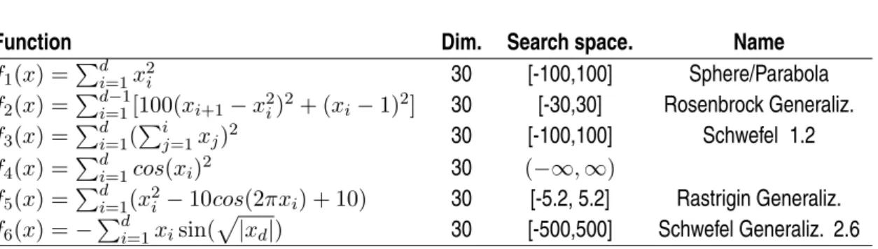
stochastic optimization techniques. They produce good results on both real life problems and optimization problems. A simple mixture between those two algorithms, called Differential Evolution - Particle Swarm Optimization (DE-PSO), is also considered. The explanation will no longer use the sine function, but the more frequently used sphere function. Also note that the explanation for this algorithm will not use a single value, but arrays (vectors) to represent particles and velocities. Therefore, it is compatible with more dimensions.
Enhanced Neural Networks
The most usual connection type in neural networks is the axo-dendritic connection. This connection is based on the fact that the axon of an afferent neuron is connected to another neuron via a synapse on a dendrite, and modelized
inANN model by a weighted activation transfer function. But, there exists many other connection types as:
axo-somatic, axo-axonic and axo-synaptic [Delacour,1987]. This paper is focused on the second kind of connection type
axo-axonic. Merely, the structure of the axo-axonic connection can be sketched by three neurons with a classical
axo-dendritic connection and the synaptic axonal termination ofN3 connected to the synapseS12. The principle
consists on propagating the action of neuronN3as synapseS12. In order to model previous connection type, two
neural networks are required [Mingo,1998]. The first (assistant) one will compute the weight matrix of the second
(principal) one. And, the second network will output a response, using the previously computed weight matrix, this
architecture is named Enhanced Neural NetworksENN[Mingo,1999;Mingo,1999a;Mingo,1999b].
Taylor Approximation
Taylor approximation degree2of a functionn-differentiable at a pointx =acan be obtained using the following
expression as a power series:
ˆ
f(x) =f(a) +f0(a)(x−a) +f
00(a)
2 (x−a)
2+e(ξ) (1)
, whereξbelongs to interval[x, a).
Iff000(x)is a continuos function in the closed interval[a, x]then this derivate has a maximunM in such interval,
and therefore, the error in the aproximation (equation1) is measure by [Blum,1991]:
maxf000(x)
≤M (2)
|e(x)| ≤ 1
6M|x−a|
3 (3)
In case an approximation degreenof functionf(x)must be obtained, previous equations can be generalized in
ˆ
f(x) =
n X
i=0
fi)(a)(x−a)i
i! +
fn+1)(ξ)(x−a)(n+1)
(n+ 1)! (4)
provided following constraints are verified:
1. fi)(x)corresponds to thei-derivate off(x). Besidesf0)(x) =f(x).
2. Ifi= 0theni! = 1.
3. ξis a point at interval[x, a).
The approximation error, that isf(x)−fˆ(x), can be measured if the (n+ 1)-derivate is a continuos function in
interval[a, x). Approximation error has a maximum defined by:
|e(x)| ≤ 1
(n+ 1)!M|x−a|
(n+1) (5)
ENN as Taylor series approximators.
Above section has shown that a function can be approximated with a given error using a polynomialP(x) = ˆf(x)
with a degreen. The errorf(x)−P(x)is measure by equation (5) in such a way that in order to find a suitable
approximation (error lower than a known threshold) it is only needed to compute sucessive derivates of function f(x)until a certain degreen.
Enhanced Neural Networks behave asn-degree polynomial approximators depending on the number of hidden
layer in the architecture. In order to obtain such behavior all activation functions of the net must be lineal function
f(x) =ax+b.
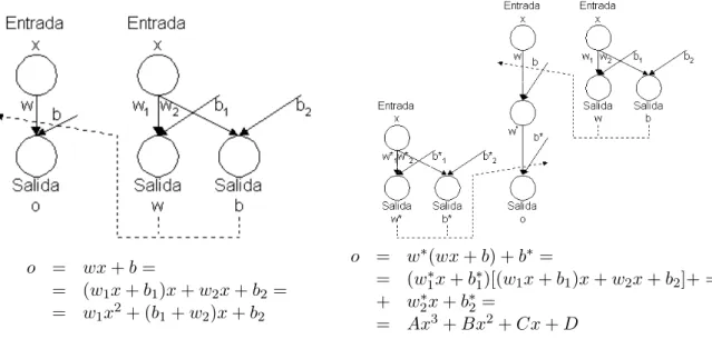
o = wx+b=
= (w1x+b1)x+w2x+b2 = = w1x2+ (b1+w2)x+b2
o = w∗(wx+b) +b∗ =
= (w∗1x+b∗1)[(w1x+b1)x+w2x+b2]+ = + w∗2x+b∗2=
= Ax3+Bx2+Cx+D
Figure 1: ENN architectures and output expressions
As shown in figure1and output equations, the number of hidden layers can be increased in order to increase the
degree of the output polynomial, that is, the numbernof hidden layers control, in some sense, the degreen+ 2of
output polynomial of the net.
Table1shows how the degree of the output polynomial increases according to the number of hidden layers in the
Table 1: Number hidden layers vs. degree of output polynomial
Hidden DegreeP(x) Output
Layers Polynomial
0 2 o=a2x2+a1x+a0
1 3 o=a3x3+a2x2+a1x+a0
· · · ·
n n+ 2 o=Pn+2
i=0 aixi
The only condition that the learning algorithm must verified is that weights must be adjusted to values related with
the sucesive derivates of functionf(x)that pattern set represents. Usually such function is unkown therefore, if
the network converges with a low mean squared error then all weights of the net have converged to the derivates of
functionf(x)(the pattern set unkown function), and such weights will gather some information about the function
and its derivates that the pattern set represents.
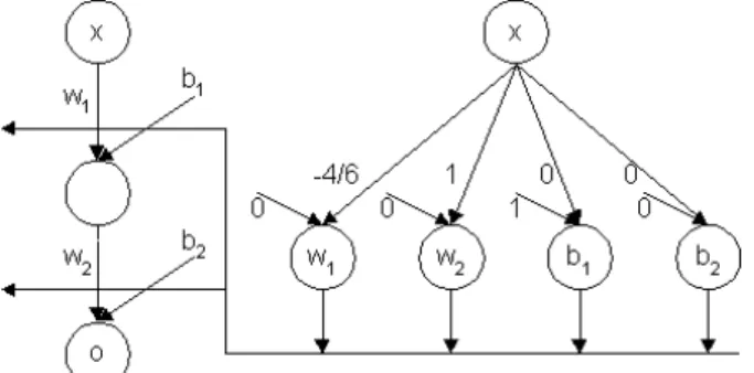
As an example, functionf(x) =sen(x)cos(x)can be approximated using equation (4), with a given pointa= 0.
Such equation can be reduced tof˜(x) = x− 64x3, using a polynomialP(x)degree 3. This is a mathematical
approach, but what happens if such function is the pattern set to an enhanced neural network mentioned before?. A one hidden layer neural network must be used in order to obtain a 3-degree polynomial as the output expression.
Figure2shows such architecture, after the training stage, the final configuration is shown. Output equation of the
net iso=x−46x3, equivalent equation withf˜(x).
Figure 2: Approximation off(x) =sen(x)cos(x)with a one hidden layer
The approximation error using net in figure2can be computed using equation (5), and thereforeM SE ≤ |e(x)|.
Such approximation is not the only one nor the best one, but it can be computed theoretically in order to provide the net some initial weights in order to speed up the learning process and to obtain a better approximation that the initial one with a lower error ratio. In sumary, Enhanced Neural Networks can be initialized to some weights computed using the Taylor Series of the function that the pattern set defines and after this initial stage the learning algorithm must be applied in order to achieved the best solution (the one that improves the Taylor Series error).
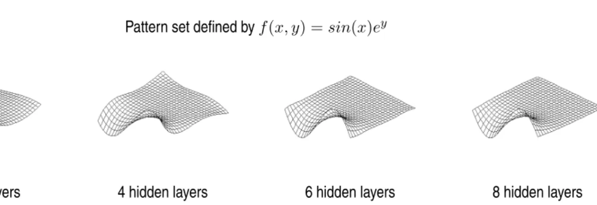
Figure3shows the surface computed by a net as the number of hidden layers is increased. The mean squared
error is decreasing as the number of hidden layers goes up. This figure shows that this kind of neural net is very suitable when approximating functions, a given function or a function defined by the pattern set.
Non-Linear Activation
According to previous ideas,linear ENNsare better than linearMLPs, or at least, they are able to generate complex
regions in order to divide the output space. When working with aMLP, only hyperplanes can be obtained. And
Pattern set defined byf(x, y) =sin(x)ey
2 hidden layers 4 hidden layers 6 hidden layers 8 hidden layers
Figure 3: Surface approximation depending on the number of hidden layers
a) Sinusoidal basis b) 3D Surfaces Approximation
Figure 4: Approximation with sinusoidal activation functions using basis of figure a).
In order to obtain a functional basis, one constraint must be made. It consists on implementing the network
architecture with linealPEs except the output neurons of assistant network. These neurons must have an activation
functiong(x)which is used to computed the functional basis as the application ofg(x)to a non lineal combination
of inputs. Figure4shows an example of a functional basis and the main network ourput.
Depending on the activation function of output neurons belonging to assistant network, the main network will output an approximation function based on non lineal combination of elements belonging to the basis. That is if a sinusoidal activation function is implemented, then a cuasi-Fourier approximation is computed by the network; is a Ridge activation function is implemented, then a cuasi-Ridge approximation is computed and so on.
Main advantage of this new approximation method is that is absolutely easy to implement. And moreover, a global approximation to all the pattern set is perform. This way, if there are enough input patterns, then the generalization error will be minimized if there are enough learning iterations.
Enhanced Neural Networks as Universal Approximators
Along the paper [Mingo,1999a], this new architecture has shown that it is very suitable when dealing with any
problem. Decision surfaces generated by the net are complex enough to represent any data set. The powerfull of these nets is in the number of hidden layers, that is, in the degree of the output polinomial associated to one output unit.
FunahashiTheorem can be directly apply toEnhanced Neural Networksin order to proof the universal approximation
property of proposed networks, provided that activation function in hidden and output neurons belongs to a given
class of functions stated byFunahashi. This way,ENNbehave as universal approximators, that is, they are able to