Dominance intensity measuring methods in MCDM with ordinal relations regarding weights

Dominance intensity measuring methods in MCDM with ordinal relations

regarding weights

A. Mateos , A. Jiménez-Martín, E.A. Aguayo, P. Sabio

Departamento de Inteligencia Artificial, Universidad Politécnica de Madrid, Campus de Montegancedo S/N, Boadilla del Monte, 28660 Madrid, Spain

a b s t r a c t

We consider a multicriteria decision-making context in which the decision-maker’s preferences are represented by a multi-attribute additive value function. We account for imprecision concerning the per-formance of alternatives, value functions and weights, which represent the relative importance of criteria. We propose two new methods based on dominance intensity measures aimed at ranking alternatives. Both methods can be applied to different representations of imprecision about weights. Their perfor-mance is compared with other existing approaches when ordinal weight information represents impre-cision concerning weights. Monte Carlo simulation is used for the comparison in terms of a hit ratio and a rank-order correlation.

1. Introduction

A key concept in Multi-Attribute Value Theory (MAVT) refers to preferential independence conditions, see Keeney and Raiffa [7]. For reasons described in Raiffa [14] and Stewart [21], the additive model is considered a valid approach in many practical situations and is widely used. The functional form of the additive model is

n

v(ai) = YwjVj(xij), (1)

where xij is the performance over the attribute (or criterion)

Xj, j = 1,..., n, for the alternative ai, i = 1,..., m; and Vj is the value

function and wj is the weight, respectively, for attribute Xj. Note that Yj=1wj — 1 and wj P 0.

However, it is often not easy to elicit precise value functions and/or values for scaling weights. They are often described within prescribed bounds or as just satisfying certain relations. Different authors refer to this situation as decision-making with imprecise

information, incomplete information or partial information [15,16].

Several reasons are given in the literature that justify why a decision maker (DM) may wish to provide imprecise information

[23,20]. For instance, regarding alternative performances, some parameters of the model may be intangible as they reflect social

* This paper was supported by the Madrid Regional Government project S-0505/ TIC/0230, the Spanish Ministry of Education and Science project TIN2008-06796-C04-02 and the Spanish Ministry of Science and Innovation project MTM2011-28983-C03-03.

* Corresponding author. Tel: +34 91 336 6596; fax: +34 91 352 4819.

E-mail addresses: [email protected] (A. Mateos), [email protected]

(A. Jiménez-Martín), [email protected] (E.A. Aguayo), [email protected] (P. Sabio).

or e n v i r o n m e n t a l impacts. Also, performance m a y b e t a k e n from statistics or m e a s u r e m e n t s , a n d t h e information t h a t w o u l d s e t t h e value of s o m e p a r a m e t e r s m a y b e incomplete, contradictory or controversial. Regarding weights, DMs m a y find it difficult t o c o m p a r e criteria or m a y n o t w a n t t o reveal their preferences in public. Moreover, t h e decision could b e taken in a g r o u p deci-sion-making situation, w h e r e imprecise information, such a s w e i g h t rankings or w e i g h t intervals, is usually derived from a negotiation process [6,11].

Many p a p e r s o n MAVT h a v e dealt w i t h imprecise information. Sage a n d W h i t e [17] proposed t h e m o d e l of Imprecisely Specified Multi-Attribute Utility Theory (ISMAUT), w h e r e preference inform a t i o n a b o u t b o t h w e i g h t s a n d utilities is n o t a s s u inform e d t o b e p r e -cise. Malakooti [ 1 0 ] suggested a n efficient algorithm for ranking alternatives w h e n t h e r e exists imprecise information a b o u t pref-erences a n d alternative values. Ahn [ 1 ] e x t e n d e d Malakooti’s work. Lee e t al. [9] e x t e n d e d t h e approach t o hierarchical s t r u c -tures, a n d Park [ 1 2 ] developed t h e concepts of weak potential optimality a n d strong potential optimality. More recently, t h e TOP-SIS m e t h o d h a s b e e n e x t e n d e d t o uncertain linguistic environ-m e n t s [25,26] o r u s e d for d e t e r m i n i n g DM w e i g h t s w i t h interval n u m b e r s [27]. Dias [ 1 9 ] provide a brief overview of a p -proaches proposed b y different a u t h o r s w i t h i n t h e MAUT (Mul-ti-Attribute Utility Theory) a n d MAVT framework t o deal w i t h imprecise information.

A recent approach t o deal w i t h imprecise information is c o m -p u t i n g different m e a s u r e s of d o m i n a n c e t o derive a ranking of alternatives, k n o w n a s dominance measuring methods. Ahn a n d Park

results of simulation experiments suggest that surrogate weighting methods, specifically the rank-order centroid weights (ROC) method, perform best in terms of selecting the best alternative and ranking alternatives.

In this paper we consider a decision-making problem with n attributes, X = {X1,... ,X„}, and m alternatives, A = {a1,..., am}, where W ( w = (w1,...,w„) e W) and V, ( v* = (vt(x1),..., Vi(xin))

e Vj) define the feasible region for scaling weights and values

associated with the alternative a, over each attribute, respectively, representing imprecise information. Therefore, Eq. (1) can be rewritten as

v(a{) = {wT v,'|w e W,v,- e V,-}.

We analyze two new dominance measuring methods based on a dominance intensity that we will denote from now on as

domi-nance intensity methods. The first method computes dominating

and dominated measures in the manner of Ahn and Park [2], but these measures are combined into a dominance intensity rather than a net dominance measure. In the second method, a global

dominance intensity measure is derived to rank alternatives. A

sim-ulation study is performed to compare the proposed methods with Ahn and Park [2] and with surrogate weighting methods and mod-ified decision rules.

The paper is organized as follows. Section 2 reviews earlier methods for dealing with imprecise information within MCDM. Section 3 introduces two dominance intensity measuring methods. Section 4 illustrates the proposed methods with an example. Sec-tion 5 uses Monte Carlo simulation to compare the performance of the proposed methods with the approaches reviewed in Sec-tion 2. We outline the conclusions in Section 6.

2. Review of earlier methods for dealing with imprecise information within MCDM

Different approaches dealing with imprecise attribute weights to output a best alternative and/or ranking of alternatives can be found in the literature. In this section, we detail the approaches that will be compared with the methods that we propose in order to analyse their performance. We start with surrogate weighting methods, which can be used when there are ordinal relations regarding attribute weights. Next, we introduce some classical decision rules modified to account for imprecise decision contexts based on the absolute dominance concept. Finally, we describe two dominance measuring methods.

2.1. Surrogate weighting methods

If the DM provides ordinal relations regarding attribute weights, i.e., we consider a ranking of importance of attributes, arranged in descending order from the most to the least important attribute, then

w e W

= w = (W1,..., w„) |W1 P W2 P • • • P w„ P 0, V~\v,- = 1

et al. [22], or rank-order centroid (ROC) weights and equal (EW)

weights, suggested by Barron and Barrett [3]. Table 1 shows how weights are computed for the above surrogate weighting methods. The ROC and RR methods typically attach more importance to the best rankings. Compared with the ROC method, the RR method distributes values more evenly over the worst rank. Thus, aggrega-tion by the RR method is insensitive to the order of the worst ranks. On the other hand, the EW method assigns equal weights to all the attributes, whereas the RS method emphasizes all the weight rank-ings at the same level (i.e., w1 — w2 = w2 — w3 = • • • = w„_1 - w„).

Surrogate weighting methods have been evaluated by differ-ent authors (see, e.g., [4]). The common conclusion reached is that the ROC method has an appealing theoretical rationale and appears to perform better than the other rank-based schemes in terms of choice accuracy. ROC has been extended to address the situation where alternative performances for an attribute are not precisely known, but again the DM has to pro-vide ordinal information [20], i.e., a ranking of alternatives for the respective attributes.

2.2. Dominance measuring methods

A possibility described in the literature for dealing with impre-cision is based on the concept of dominance. Given two alternatives

ak and a,, alternative ak dominates a, if Dkj P 0, with Dkj being the optimum value of the optimization problem,

Dkj = min{v(ak) - v(aj) = wT\k - wT v,|w e W,\k e Vk,\j e Vj}, (2) and there exists at least one w, \k and v, such that the overall value of ak is strictly greater than that of a,. This concept of dominance is called pairwise dominance.

Another type of dominance, known as absolute dominance [18], can be employed. Absolute dominance considers the following optimization problems:

Uk = max {w TVt|w e W,vt e Vt} and

Lk = min {w TVt|w eW,\k eVk}.

Alternative ak dominates absolutely a, if Lk P Vj. Note that if ak absolutely dominates a,, then ak dominates a,, but the reverse does not hold.

This dominance approach often results in almost no priorization of alternatives or too many non-dominated alternatives [8]. How-ever, pairwise and absolute dominance values can be used to further prioritize competitive alternatives, and hence recommend the best alternative and fully rank alternatives. The use of these dominance values is exemplified by the modification of four classical decision rules to encompass an imprecise decision context [13,18]:

• maximax or optimist rule (OPT) consists of evaluating each alter-native based on its maximum guaranteed value, i.e., best case =• maximax: maxj{Uj}.

• maximin or pessimist rule (PES) consists of evaluating each alter-native based on its minimum guaranteed value, i.e., worst case =• maximin: max,{L,}.

Surrogate weighting methods deal w i t h r a n k e d a t t r i b u t e w e i g h t s t o o u t p u t a b e s t alternative a n d / o r ranking of alternatives. In t h e s e m e t h o d s , a w e i g h t vector is selected from a s e t of admissible w e i g h t s t o r e p r e s e n t t h e set. This vector is t h e n u s e d t o evaluate t h e alternatives b y m e a n s of t h e m u l t i - a t t r i b u t e value m o d e l . Commonly u s e d surrogate weighting m e t h o d s a r e rank sum (RS) weights a n d rank reciprocal (RR) weights, proposed i n Stillwell

T a b l e 1

S u r r o g a t e w e i g h t i n g m e t h o d s .

R a n k s u m w e i g h t s

R a n k r e c i p r o c a l w e i g h t s

R a n k - o r d e r c e n t r o i d w e i g h t s E q u a l w e i g h t s

(RS)

(RR)

(ROC)

(EW)

£ j - 1 "(n+ 1 )

Wv = ^1 l, ! = 1 , . . . , n

W; = ^ ^ , i = 1 , . . . , n

• minimax regret rule (REG) consists of evaluating each alternative based on the maximum loss of value with respect to a better alternative =$- minimax regret: mink{MRk}, where MRk repre-sents the maximum regret incurred when choosing alternative

ak, i.e.,

MRk = max { max{w Tv, - w T\k | w e W, v,- e Vj,\k e Vk }Vj ¥=k}. • central value rule (CEN) consists of evaluating each alternative

based on the midpoint of the range of possible

perfor-3 . C o m p u t e t h e ratio

mances =$• central values: maxk ^ ± M .

Obviously none of these rules ensures that the best-ranked alternative coincides. However, simulations show that the selected alternative is generally one of the best [19].

A more recent approach is computing different measures of dominance to derive a ranking of alternatives, known as dominance

measuring methods. For instance, Ahn and Park [2] compute a dom-inating measure <pt = S-1Ag and a dominated measure

<pk = ^j-1^jk for alternative ak, and then derive a net dominance as 4k = 4t~4k. With these measures, Ahn and Park proposed two methods:

j T

Note that R£ is well defined because we can assume that 0 < 4>k> - 4>k<, avoiding division by 0, as demonstrated at the end of the algorithm. Note also that 0 < R£ < 1.

4. Compute the dominated indices tp^tp^< and tp^ for each alter-native ak:

m m m

4>

= y^Pjk, 4k> = y2Dj

, and

4^

= V ^ , k = 1 , . . . ,m.

Dii, > 0

j – k D < 0 _jk

In other words, <pk is computed by adding the paired dominance values in the fcth column of D, whereas ip^> and 4>k < are computed

in the same way, but considering just the positive and negative val-ues in the respective column. Note that 4>k = 4k> + 4k<.

5. Compute the ratio

Rl

if

• API: Rank alternatives according to <pt values, where the pro-posed alternative is that for which <pk is maximum.

• AP2: Rank alternatives according to <j>k. 3. Dominance intensity measuring methods

We introduce two new dominance measuring methods based on dominance intensities, denoted dominance intensity measuring

methods. The first one is based on the same idea as Ahn and Park

[2]. It also computes dominating and dominated measures but they are combined into a dominance intensity rather than a net domi-nance index. In the second method, a global domidomi-nance intensity in-dex is derived to rank alternatives. These are used as a measure of the strength of the preference in the sense that a greater value is better.

3.1. Dominance intensity method 1 (DIM1)

DIM1 is implemented as follows:

1. Obtain the paired dominance values Dki by solving problem Eq.

(2) for m(m - 1) ordered pairs of alternatives, grouped in the matrix:

D

£>12 E>21

i-'m1 L*m2

D 1(m-1)

D 2(m-1)

£*3(m-1)

An(m-1)

i-'2m

2 . C o m p u t e t h e dominating indices native ak:

P+> and k < for each

alter-\ L)bi k+> _{y^Dfy, and4£}

< = y^Dkj, k = 1,...,m.

i=1

D H > 0

j – k D < 0 _kj

In other words, 4>k is computed adding the paired dominance values in the fcth row of D, whereas <^> and (pt< are computed in the same way, but just considering positive and negative values in the corre-sponding row, respectively. Clearly, 4>k = 4V> +

that 0 < (p^ - (p^, and 0 < Kj~ < 1.

6. Calculate the global dominance intensity value Dk for each alter-native ak:

Dk = Rk n - k = 1 , . . . , m.

Note that - 1 < Dk < 1, where - 1 = Dk ^^> Vjk when all alternatives dominate ak, and Dk =

(R+ = 0 and Rk

1

_(K

1) 1

and Rk = 0) when all alternatives are dominated by ak.

7. Rank alternatives according to Dk values, where the best alter-native is that for which Dk is maximum and the worst is that for which Dk is minimum.

Let us demonstrate that Rk is well defined. Rk would not be well defined if tp^ - 4k< = 0. In this case,

rk

i'V

= 0 =^

r.

=> wT\k - wTy, P 0, Vj, Vw => wTy, - wT\k < 0, Vj => Djk < 0, Vj. Therefore, we have two possibilities:

• Dkj = 0,Vj and Djk < 0,Vj =$- alternative ak dominates aj,\/j =$- ak is the most preferred alternative. This may be recognized from the beginning, so we assume it does not happen.

• Dkj = 0, Vj and Djk = 0,Vj =• wT\k = wT v,Vw e W =• Both alter-natives are indifferent. In this case, we can discard alternative a, and keep ak (or the opposite).

As a conclusion, if we assume that there are no two alternatives

ak and a, with wTyk =wTYj\/w eW,\/yk eVk,\/\j eVj, (in this case, alternative a,, or alternative ak, would be discarded because they are indifferent) and <pk> - 4k< = 0, then alternative ak domi-nates a,, i.e., alternative ak is preferred, and a, would be eliminated from the analysis.

The difference between this approach and the methods pro-posed by Ahn and Park is as follows. Ahn and Park’s first method,

AP1, adds positive and negative values for the alternative in its

respective row. This accounts for the dominance of this over the other alternatives. Likewise, Ahn and Park’s second method, AP2, adds positive and negative values to both the row and column. The two quantities are then subtracted. The values added in the column account for the dominance of the other alternatives over Note that Rk is also well defined because we can assume

the alternative in question. As pointed out in Section 2, a simula-tion study showed AP1 to be better than AP2. The reason is that

AP2 uses duplicate information (row and column values).

The starting point for DIM1 is AP2. The aim is to improve AP2 by reducing the duplicate information involved in the computa-tions. We have taken into account that a given alternative, ak, only dominates alternatives with positive elements in the feth row of the dominance matrix. Analogously, this alternative is dominated only by alternatives with positive elements in the feth column.

Therefore, we compute the dominating measure by adding positive values in the respective row, which we divide by the dif-ference between the sums of the positive and negative values in that row. Likewise, we compute the dominated measure by adding positive values in the respective column, which we divide by the difference between the sums of the positive and negative values in that column.

This type of ratios attach more weight to positive values in the row (or column). This means that DIM1 would output a value greater than zero in the event of positive values being canceled out by negative values where the dominating (dominated) mea-sures in AP1 and AP2 would be zero.

However, DIM1 has a drawback: if all the elements in D are neg-ative then it is not possible to derive a ranking of alternneg-atives be-cause their dominance intensity is zero in all cases, since tp^ = 0 a n d 0;Vfc. This drawback implies that DIM1 is not indepen-dent of irrelevant alternatives. A simple numerical example fol-lows. Consider a two-criteria problem. The only constraints on weights are that they should be non-negative and add up to 1. Alternatives are a1 = (e; 1 +e);a2 = (0;1) and a3 = (1;0) (e is a number between 0 and 1). Considering all three alternatives, a1 is the best-ranked according to DIM1. But this is because we have included a2, which is irrelevant. If we remove a2, DIM1 is unable to rank the alternatives. In Section 3.2, we propose another domi-nance intensity method that overcomes this drawback.

3.2. Dominance intensity method 2 (DIM2)

To introduce the second dominance intensity method, D1M2, we observe that, trivially,

Dkj < w T(yk - V,) < -Djk; Vw e W; Vt e Vk;\j e V,:

In this method, paired dominance values Dkj are first transformed into dominance intensities Dlkj. Then, a global dominance intensity

(GDIk) is derived for each alternative ak. This is used as a measure of the strength of preference, in the sense that a greater global dom-inance intensity is better.

DIM2 is implemented as follows:

1. Obtain matrix D as before.

2. If Dkj P 0, then alternative ak dominates alternative a,, and we say that the dominance intensity of ak over a, is 1, i.e., Dlkj = 1. E l s e (Dkj < 0 ) :

- If Djk P 0, then alternative a, dominates alternative ak, and we say that the dominance intensity of ak over a, is 0, i.e.,

DIkj = 0.

- Else, (Djk < 0) the dominance intensity of ak over a, is defined as

DIkj -D jk -Djk - Dkj :

3. Calculate a global dominance intensity (GDI) for each alterna-tive ak

m

GDIk = V" DIkj:

4. Rank alternatives according to the GDIk values, where the best (rank 1) is the alternative for which GDIk is maximum and the worst is the alternative for which GDIk is minimum.

In Section 5, we analyse the performance of the proposed meth-ods and compare them with other methmeth-ods reviewed in Section 2.

4. A numerical example

In this section, we provide a simple example to illustrate the proposed dominance intensity measuring methods. Let us consider a decision-making problem with five attributes, X,; i = 1;...; 5 and five alternatives, a,;j = 1;... ;5. We assume that the ranking of attribute importance is 1 P W1 P w2 P w3 P w4 P w5 P 0, with ]T5=1W; = 1.

The evaluation of the five alternatives is as follows

0.2 O3 0,4

as

X\ X2 X3 Xi X§ / 0.711 0.146 0.115 0.892 0.241 \

0.253 0.192 0.087 0.722 0.477 0.401 0.805 0.524 0.327 0.828 0.793 0.965 0.647 0.241 0.091 ^ 0.284 0.576 0.714 0.618 0.411 J

F o r c o n v e n i e n c e , t h e c o l u m n s i n t h i s m a t r i x a r e n o r m a l i z e d s o

t h a t t h e s m a l l e s t v a l u e i s z e r o a n d t h e l a r g e s t v a l u e i s o n e :

0:848 0 0:044 1 0:203

0 0:056 0 0:739 0:523

0:4274 0:804 0:697 0:132 1

1 1 0 : 8 9 3 0 0 CA

0:057 0:525 0:714 1 0:434

O p t i m i z a t i o n p r o b l e m s a r e s o l v e d t o c o m p u t e p a i r e d d o m i -n a -n c e v a l u e s , l e a d i -n g t o t h e c o r r e s p o -n d i -n g d o m i -n a -n c e m a t r i x :

DI--In the DIM1 method, the dominating measures, 4>k> and 4>k<, are computed for each alternative, followed by the ratios Rk, see

Table 2. For instance, 4%> = 0:152 + 0:3148 + 0:0596 = 0:5264 or

4>t/< = -0:574 - 0:726 - 0:0633 = -1:3633. Next, the dominated

measures 4>k< and <pk> are computed for each alternative, followed by the proportion Rk, shown in Table 2.

Finally, the ranking of alternatives is derived from the global

dominance intensity Dk, see Table 3.

In the DIM2 dominance intensity measuring method, once the paired dominance matrix D is available, dominance intensities Dlkj are computed, leading to the matrix:

ai

02 "3 CZ4 05

{ ~

0

0.34

1

^ 0.22

1

-1 1 1

0.66

0

0 0

0,004

-0

0.77 \

0

0.80

1

" /

Ol 02 03 04 05

( ~ 0

0.34

1

^ 0.22

1

-1 1 1

0.66

0

0 0

0,004

-0

0.77 \

0

0.80

1

" /

DI--Table 2

Dominating and dominated measures.

Dominating measures Dominated measures

Altern. Ri Altern. R:

a1 a2 a3 a4 a5

0.155 —1.1907 0.11518 a1

0 -2.93 0 a2

0.274 —1.3633 0.16734 03 0.5264 —0.003 0.99433 a4 0.057 -1.9826 0.02794 0 5

Table 3

Global dominance intensities and ranking with DIM1.

a1 a2 a3

D& 0.05 —1 0.17 Ranking 3 5 2

a4

0.99 1

0 5 -0.04 4

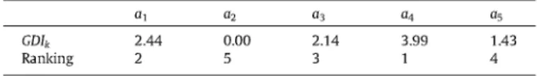
Table 4

Global dominance intensities and ranking with DIM2.

a1 a2 a3

GDIk 2.44 0.00 2.14

Ranking 2 5 3 a4

3.99 1

a5

1.43 4

For instance, as D12 =0:155 P 0,thena1 dominates a2 and D/12 = 1. On the other hand, D14 = -0:6667 < 0, whereas D41 =0:152 > 0, so D/14 = 0.

Finally, D13 = -0:2943 < 0 and D31 = -0:574 < 0. Conse-quently, D/13 = 029435+0 574 = 0:66.

Finally, the ranking of alternatives is derived from the global dominance intensity GDIk (see Table 4).

We find that the rankings output by both methods (D/M1 and D/M2), see Tables 3 and 4, are very similar but do not match ex-actly. The best- and worst-ranked alternatives are the same for both methods (a4, and a5 and a2, respectively). However, the alter-natives ranked second and third are different for each method (a1 and a3, respectively). The question is, then, does one method out-perform the other for different decision-making settings, i.e., for a different number of attributes or alternatives?

5. Performance analysis based on Monte Carlo simulation Having described the dominance intensity measuring methods we propose ( DIM1 and DIM2), let us now compare these methods with Ahn and Park’s approach, surrogate weighting methods and decision rules modified to encompass an imprecise decision-mak-ing context. Note that, although DIM1 could be discarded from fur-ther analysis since it is not independent of irrelevant alternatives, as explained in Section 3.1, it has been considered in the simula-tion process.

The proposed methods can be applied for different representa-tions of imprecision concerning weights. In surrogate weighting methods, however, DMs provide ordinal relations regarding attri-bute weights. For comparability, we have considered ordinal rela-tions about weights throughout the simulation.

We shall carry out a simulation study of the above methods to analyze their performance. For a decision-making problem with m alternatives and n attributes, the process would be as follows:

1. Component utilities are randomly generated for each alterna-tive in each attribute from a uniform distribution in (0,1), lead-ing to an m x n matrix. The columns in this matrix are normalized to make the smallest value zero and the largest value one, and dominated alternatives are removed. Note that these alternatives are removed in the simulation because they are not useful for analyzing the performance of the considered methods.

2. Attribute weights are randomly generated according to the ranking of attribute importance [5]. If these weights are the

TRUE weights, the derived ranking of alternatives will be

denoted as the TRUE ranking. To generate the TRUE weights, first select n - 1 independent random numbers from a uniform dis-tribution on (0,1), and rank these numbers. Suppose the ranked numbers are 1 P r„_1 P • • • P r2 P n > 0. The differences between adjacently ranked numbers are then used as the target

weights w\ = 1 - r„_1, w£_1 = r„_1 - r„_2 ,...,w1 = r1. The resulting weights will sum 1 and be uniformly distributed in the weight space. Attribute weights corresponding to surrogate weighting methods are computed as described in the introduction.

3. The ranking of alternatives is computed for each method (surro-gate weighting methods, modified decision rules and domi-nance measuring methods) according to their procedures and compared with the TRUE ranking, computed in the last step. We use two measures of efficacy, the hit ratio and rank-order

correlation [3,2]. The hit ratio is the proportion of cases in which the method selects the same best alternative as in the TRUE

ranking. Rank-order correlation represents how similar the

overall rank structures of alternatives are in the TRUE ranking and in the ranking derived from the method. It is calculated using Kendall’s T [24]:

2 x (number of pairwise preference violations)

T = 1 " Total number of pair preferences

= , V^, (3)

m(m - )/2

where S is the difference between the number of concordant (or-dered in the same way) and discordant (or(or-dered differently) pairs and m is the total number of alternatives.

If there are tied (same value) observations then the denominator

m{m - 1)/2 has to be replaced by

^ [ m ( m - 1 ) / 2 - £ j 1m-1)/2] [ m ( m - 1 ) / 2 - ^ ^ - 1 ) / 2 ,

where t, is the number of observations tied at the TRUE ranking, and u, is the number of observations tied at the ranking derived from the method.

Like Ahn and Park [2], we validated the results using four differ-ent levels of alternatives (m = 3,5,7,10 ) and five differdiffer-ent levels of attributes (n = 3,5,7,10,15). Also, 10 replications of 10,000 tri-als were performed for each of the 20 design elements (alternatives x attributes). Replications were parallelized to save computational resources (mainly time).

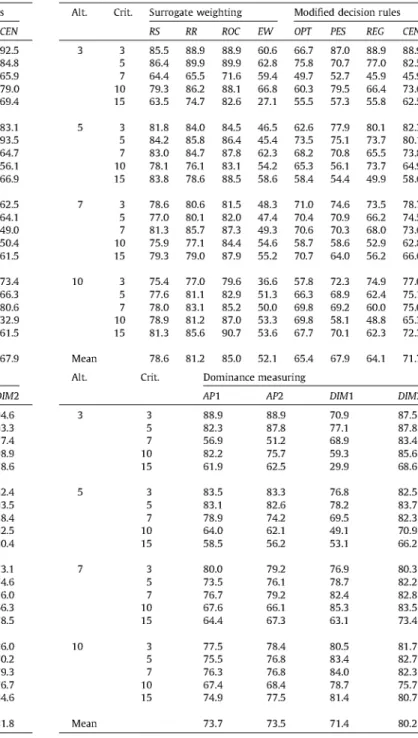
Table 5 exhibits the average hit ratio for each of the 20 design elements, i.e., the average values of 10 replications of 10,000 trials, whereas the last row in this table is the mean of each column.

Looking at the surrogate weighting methods, ROC is the best, followed by the RR method, the RS method and the EW method. This result matches those reported in Barron and Barrett [3] and Ahn and Park [2]. Regarding modified decision rules, although there is no regular trend, the PES method appears to be better than the CEN method. CEN outperforms the REG method, and REG out-performs the OPImethod. In any case, modified decision rules are worse than surrogate weighting methods, except for the EW meth-od. For the dominance intensity methods, the mean value for the

DIM2 method is the highest (81.8), its hit ratio being the highest

for 13 out of the 20 design elements. The DIM2 method is followed by DIM1, which is better thanAPJ. API is better than AP2.

On the whole, ROC and DIM2 are better than the other methods in terms of hit ratio. The DIM2 method performs better than the dominance measuring methods in Ahn and Park [2], and outputs results closer to the ROC method. Furthermore, according to the paired-samples t-test (which computes the difference between the mean values of the two methods and tests whether the average differs from zero), there is no significant difference among the hit ratio means for the DIM2 and ROC methods (significance level, two-tailed: 0.210).

ROC is again the best surrogate weighting method in terms of

Table 5 Average hit ratios.

Table 6

Rank-order correlation (Kendall’s s).

Alt. Crit. Surrogate weighting Modified decision rules

10

Mean

Alt.

10

Mean

RS RR ROC EW OPT PES REG CEN

3 89.6 5 82.5 7 79.4 10 94.8 15 78.2 3 82.4 5 93.5 7 90.9 10 78.3 15 89.3 3 63.0 5 68.8 7 84.6 10 64.7 15 71.7 3 73.4 5 72.2 7 72.9 10 76.7 15 80.7 79.94 Crit.

92.5 92.5 89.6 77.1 89.6 92.5 92.5 88.0 88.0 81.2 74.8 81.4 84.8 84.8 78.4 79.9 73.4 56.0 73.5 65.9 65.9 94.8 94.8 84.8 59.1 94.8 75.1 79.0 87.8 90.1 57.1 53.8 71.7 69.4 69.4

83.1 84.4 53.9 46.6 65.0 84.4 83.1 93.5 93.5 38.3 62.2 83.8 93.5 93.5 90.9 90.9 71.2 44.7 84.8 70.2 64.7 64.3 79.2 59.9 29.5 56.7 58.4 56.1 85.1 91.1 59.5 46.9 81.3 58.9 66.9

65.7 66.6 45.1 36.1 60.8 64.9 62.5 71.4 77.2 47.9 42.6 71.4 61.8 64.1 84.6 84.6 43.5 39.8 72.1 66.3 49.0 64.2 72.3 48.7 40.8 51.7 49.2 50.4 78.5 87.8 50.0 51.5 80.2 53.2 61.5

73.4 73.4 42.2 37.9 53.0 65.0 73.4 66.2 72.0 30.4 42.1 55.4 66.4 66.3 80.6 80.6 32.6 31.4 80.6 67.7 80.6 76.7 88.3 58.4 14.0 62.2 47.1 32.9 82.4 85.7 78.0 22.2 81.2 60.4 61.5

80.1 83.6 57.3 45.6 72.5 67.7 67.9

Dominance measuring

AP1 AP2 DJM1 DIM2

3 5 7 10 15 3 5 7 10 15 3 5 7 10 15 3 5 7 10 15 92.5 84.8 74.4 88.7 78.6 82.4 93.5 88.4 73.0 82.7 65.7 67.4 80.1 62.2 78.5 69.6 68.1 76.7 73.2 80.0 78.0 92.5 84.8 65.9 79.0 69.4 84.4 93.5 64.7 41.8 66.9 66.5 68.7 66.3 61.1 61.5 73.4 66.2 71.5 48.0 73.7 70.0 89.6 94.2 95.3 96.7 84.8 76.8 72.9 88.4 85.3 95.7 64.0 73.0 70.3 57.8 56.5 70.4 68.2 72.7 81.2 80.0 78.7 94.6 93.3 77.4 98.9 78.6 82.4 93.5 88.4 82.5 80.4 73.1 74.6 76.0 66.3 78.5 86.0 70.2 79.3 76.7 84.6 81.8 Alt. 3 5 7 10 Mean Alt. 3 5 7 10 Mean Crit. 3 5 7 10 15 3 5 7 10 15 3 5 7 10 15 3 5 7 10 15 Surrogate weighting

RS RR ROC

85.5 86.4 64.4 79.3 63.5 81.8 84.2 83.0 78.1 83.8 78.6 77.0 81.3 75.9 79.3 75.4 77.6 78.0 78.9 81.3 78.6 Crit. 3 5 7 10 15 3 5 7 10 15 3 5 7 10 15 3 5 7 10 15 88.9 88.9 89.9 89.9 65.5 71.6 86.2 88.1 74.7 82.6 84.0 84.5 85.8 86.4 84.7 87.8 76.1 83.1 78.6 88.5 80.6 81.5 80.1 82.0 85.7 87.3 77.1 84.4 79.0 87.9 77.0 79.6 81.1 82.9 83.1 85.2 81.2 87.0 85.6 90.7 81.2 85.0 EW 60.6 62.8 59.4 66.8 27.1 46.5 45.4 62.3 54.2 58.6 48.3 47.4 49.3 54.6 55.2 36.6 51.3 50.0 53.3 53.6 52.1

Modified decision rules

OPT 66.7 75.8 49.7 60.3 55.5 62.6 73.5 68.2 65.3 58.4 71.0 70.4 70.6 58.7 70.7 57.8 66.3 69.8 69.8 67.7 65.4 Dominance measuring AP1 88.9 82.3 56.9 82.2 61.9 83.5 83.1 78.9 64.0 58.5 80.0 73.5 76.7 67.6 64.4 77.5 75.5 76.3 67.4 74.9 73.7 AP2 88.9 87.8 51.2 75.7 62.5 83.3 82.6 74.2 62.1 56.2 79.2 76.1 79.2 66.1 67.3 78.4 76.8 76.8 68.4 77.5 73.5 PES 87.0 70.7 52.7 79.5 57.3 77.9 75.1 70.8 56.1 54.4 74.6 70.9 70.3 58.6 64.0 72.3 68.9 69.2 58.1 70.1 67.9 DJM1 70.9 77.1 68.9 59.3 29.9 76.8 78.2 69.5 49.1 53.1 76.9 78.7 82.4 85.3 63.1 80.5 83.4 84.0 78.7 81.4 71.4 REG 88.9 77.0 45.9 66.4 55.8 80.1 73.7 65.5 73.7 49.9 73.5 66.2 68.0 52.9 56.2 74.9 62.4 60.0 48.8 62.3 64.1 CEN 88.9 82.5 45.9 73.6 62.5 82.3 80.1 73.8 64.9 58.6 78.7 74.5 73.6 62.8 66.6 77.0 75.1 75.0 65.3 72.3 71.7 DIM2 87.5 87.8 83.4 85.6 68.6 82.5 83.7 82.3 70.9 66.2 80.3 82.2 82.8 83.5 73.4 81.7 82.7 82.3 75.7 80.7 80.2

In t h e ROC m e t h o d , t h e rank-order correlations r a n g e from 71.6% t o 90.7%, a n d t h e values a r e relatively constant irrespective of t h e n u m b e r of alternatives ( m e a n values a r e 84.2%, 86%, 84.6% a n d 85% for 3 , 5, 7 a n d 1 0 alternatives, respectively). W i t h exception of EW, modified decision rules a r e w o r s e t h a n t h e surrogate weighting m e t h o d .

As regards d o m i n a n c e intensity m e a s u r i n g m e t h o d s , DIM2 p e r -forms b e t t e r t h a n DIM1 a n d t h e approaches suggested by Ahn a n d Park [2], a n d reaches a rank-order correlation close t o t h e ROC m e t h o d . Its rank-order correlations range from 66.2% t o 87.8%, a n d a r e relatively constant irrespective of t h e n u m b e r of alterna-tives ( m e a n values a r e 82.6%, 77.1%, 80.4% a n d 80.6%, respectively). In this case, t h e paired-samples t-test s h o w s a significant difference a m o n g t h e rank-order correlation m e a n s for t h e DIM2 a n d ROC m e t h o d s (significance level, t w o - t a i l e d : 0.009). On t h e o t h e r h a n d ,

DIM1 h a s t h e w o r s t rank-order correlation m e a n o u t of all t h e d o m i n a n c e intensity m e a s u r i n g m e t h o d s , this value improves in proportion t o t h e n u m b e r of alternatives r a n k e d ( m e a n values for 3 , 5, 7 a n d 1 0 alternatives a r e 61.2%, 65.3%, 77.3% a n d 81.6%, respectively), s e e Table 6.

Note t h a t ROC is a n e x a m p l e of centroid values, w h i c h gener-alizes t o any convex value set defined by linear inequalities, a n d centroid c o m p u t a t i o n s a r e relatively straightforward for a large class of situations. However, w e think t h a t DIM2 is m o r e gener-ally applicable in t h e s e n s e t h a t , it is easy t o apply e v e n t o a nonconvex value set (corresponding t o different t y p e s of i m p r e cision concerning t h e i n p u t parameters), once t h e respective o p t i -mization p r o b l e m s h a v e b e e n solved (possibly based o n t h e application of metaheuristics) a n d t h e d o m i n a n c e m a t r i x h a s b e e n obtained.

6. Conclusions

In complex decision-making problems it is often not easy to eli-cit precise values for scaling weights representing the relative importance of criteria, which are described by a constraint set, for instance, within prescribed bounds or as just satisfying certain ordinal relations (ranked attribute weights).

Two distinct approaches for suggesting an alternative and/or ranking of alternatives can be found in the literature dealing with ranked attribute weights. One group is the so-called surrogate weighting methods, where a weight vector is selected from a set of admissible weights to represent that set. This vector is then used to evaluate the alternatives by means of a multi-attribute value model. The other possibility is to eliminate inferior alternatives based on the concept of dominance. An example of the employment of dominance values is the modification of classical decision rules to encompass an imprecise decision context. A more recent ap-proach is to use information about each alternative’s intensity of dominance, known as dominance intensity measuring methods.

We have proposed two new dominance intensity measuring methods, DIM1 and DIM2. DIM1 is designed to improve one of the methods proposed by Ahn and Park, AP2, by reducing duplicate information to compute dominating and dominated measures. These measures are then combined to yield a dominance intensity. However, DIM1 was dispensed with because it is not independent of irrelevant alternatives. DIM2 derives a global dominance intensity measure to rank alternatives.

Monte Carlo simulation techniques have been used to analyse the performance of the proposed methods and to compare them with dominance measuring methods proposed by other authors (Ahn and Park), surrogate weighting methods and adapted decision rules.

As regards average hit ratios, DIM2 and ROC outperform the other methods (including DIM1) and, according to the paired-sam-ples t-test, there is no significant difference among them. DIM2 and ROC also outperform the other methods (including DIM1) in terms of rank-order correlation, but ROC slighty outperforms DIM2 in this case.

Note, however, that ROC can be only applied when ordinal rela-tions regarding attribute weights are provided. However, DIM2 is more generally applicable since it can also be used when the imprecision concerning weights or even value functions is repre-sented in other ways, for example by interval values, probability distributions or even fuzzy numbers. And again it is applicable when there is uncertainty about the alternative performances.

References

[1] B.S. Ahn, Extending Malakooti’s model for ranking multicriteria alternatives with preference strength and partial information, IEEE Trans. Syst., Man. Cyb.: Part A 33 (2003) 281–287.

[2] B.S. Ahn, K.S. Park, Comparing methods for multiattribute decision making with ordinal weights, Comput. Oper. Res. 35 (2008) 1660–1670.

[3] F. Barron, B. Barrett, Decision quality using ranked attribute weights, Man. Sci. 42 (1996) 1515–1523.

[4] J. Butler, D.L. Olson, Comparison of centroid and simulation approaches for selecting sensitivity analysis, J. Multi-Crit. Decis. Anal. 8 (1999) 146–161.

[5] J. Jia, G.W. Fischer, J.S. Dyer, Attribute weighting method and decision quality in the presence of response error: A simulation study, J. Behav. Decis. Making 1 1 (1998) 85–105.

[6] A. Jiménez, A. Mateos, S. Ríos Insua, Monte Carlo simulation techniques in a decision support system for group decision-making, Group Dec. Negot. 14 (2005) 109–130.

[7] R.L. Keeney, H. Raiffa, Decision with Multiple Objectives: Preferences and Value-Tradeoffs, Wiley, New York, 1976.

[8] C.W. Kirkwood, J.L. Corner, The effectiveness of partial information about attribute weights for ranking alternatives in multiattribute decision making, Org. Behav. Human Dec. Proc. 54 (1993) 456–476.

[9] K. Lee, K.S. Park, H. Kim, Dominance, potential optimality, imprecise information and hierarchical structure in multi-criteria analysis, Comput. Oper. Res. 29 (2002) 1267–1281.

[10] B. Malakooti, Ranking and screening multiple criteria alternatives with partial information and use of ordinal and cardinal strength of preferences, IEEE Trans. Syst., Man. Cyb.: Part A 30 (2000) 787–801.

[11] A. Mateos, A. Jiménez, S. Ríos Insua, Monte Carlo simulation techniques for group decision-making with incomplete information, Euro. J. Oper. Res. 174 (2006) 1842–1864.

[12] K. Park, Mathematical programming models for characterizing dominance and potential optimality when multicriteria alternative values and weights are simultaneously incomplete, IEEE Trans. Syst., Man. Cyb.: Part A 34 (2004) 601– 614.

[13] J. Puerto, A.M. Marmol, L. Monroy, F.R. Fernández, Decision criteria with partial information, IEEE Trans. Oper. Res. 7 (2000) 51–65.

[14] H. Raiffa, The Art and Science of Negotiation, Harvard University Press, Cambridge, 1982.

[15] D. Ríos Insua, Sensitivity Analysis in Multi-objective Decision Making, Springer, New York, 1990.

[16] D. Ríos, S. French, A framework for sensitivity analysis in discrete multi-objective decision-making, Euro. J. Oper. Res. 54 (1991) 176–190.

[17] A. Sage, C.C. White, Ariadne: a knowledge-based interactive system for planning and decision support, IEEE Trans. Syst., Man. Cyb.: Part A 14 (1984) 35–47.

[18] A. Salo, R.P. Hämäläinen, Preference ratio in multiattribute evaluation (PRIME) - elicitation and decision procedures under incomplete information, IEEE Trans. Syst., Man. Cyb.: Part A 3 1 (2001) 533–545.

[19] P. Sarabando, L.C. Dias, Multi-attribute choice with ordinal information: a comparison of different decision rules, IEEE Trans. Syst., Man. Cyb.: Part A 39 (2009) 545–554.

[20] P. Sarabando, L.C. Dias, Simple procedures of choice in multicriteria problems without precise information about the alternatives values, Comput. Oper. Res. 37 (2010) 2239–2247.

[21] T.J. Stewart, Robustness of additive value function method in MCDM, J. Multi-Crit. Decis. Anal. 5 (1996) 301–309.

[22] W.G. Stillwell, D.A. Seaver, W.A. Edwards, Comparison of weight approximation techniques in multiattribute utility decision making, Org. Behav. Human Decis. Proc. 28 (1981) 62–77.

[23] M. Weber, Decision making with incomplete information, Euro. J. Oper. Res. 28 (1987) 44–57.

[24] R.L. Winkler, W.L. Hays, Statistics: Probability, Inference and Decision, Holt, Rinehart & Winston, New York, 1985.

[25] Z. Xu, A method for multiple attribute decision making with incomplete weight information in linguistic setting, Knowl.-Based Syst. 20 (2007) 719– 725.

[26] Y. Xu, Q. Da, A method for multiple attribute decision making with incomplete weight information under uncertain linguistic environment, Knowl.-Based Syst. 2 1 (2008) 837–841.