sensors
ISSN 1424-8220 www.mdpi.com/journal/sensors
Article
A Novel Topology Control Approach to Maintain the Node
Degree in Dynamic Wireless Sensor Networks
Yuanjiang Huang *, Jos´e-Fern´an Mart´ınez, Vicente Hern´andez D´ıaz and Juana Sendra
Centro de Investigaci´on en Tecnolog´ıas Software y Sistemas Multimedia para la Sostenibilidad (CITSEM), Campus Sur Universidad Polit´ecnica de Madrid (UPM), 28031 Madrid, Spain; E-Mails: [email protected] (J.-F.M.); [email protected] (V.H.D.);
[email protected] (J.S.)
*Author to whom correspondence should be addressed; E-Mail: [email protected]; Tel.: +34-91-336-5511; Fax: +34-91-336-7817.
Received: 25 December 2013; in revised form: 20 February 2014 / Accepted: 24 February 2014 / Published: 7 March 2014
Abstract: Topology control is an important technique to improve the connectivity and the reliability of Wireless Sensor Networks (WSNs) by means of adjusting the communication range of wireless sensor nodes. In this paper, a novel Fuzzy-logic Topology Control (FTC) is proposed to achieve any desired average node degree by adaptively changing communication range, thus improving the network connectivity, which is the main target of FTC. FTC is a fully localized control algorithm, and does not rely on location information of neighbors. Instead of designing membership functions and if-then rules for fuzzy-logic controller, FTC is constructed from the training data set to facilitate the design process. FTC is proved to be accurate, stable and has short settling time. In order to compare it with other representative localized algorithms (NONE, FLSS, k-Neighbor and LTRT), FTC is evaluated through extensive simulations. The simulation results show that: firstly, similar to k-Neighbor algorithm, FTC is the best to achieve the desired average node degree as node density varies; secondly, FTC is comparable to FLSS and k-Neighbor in terms of energy-efficiency, but is better than LTRT and NONE; thirdly, FTC has the lowest average maximum communication range than other algorithms, which indicates that the most energy-consuming node in the network consumes the lowest power.
1. Introduction
Topology control has been proposed as a technique to address many problems in networks by adding or deleting nodes/links according to certain algorithms/protocols, with the aim of obtaining expected network properties. In Wireless Sensor Networks (WSNs), the topology control is usually achieved by means of changing the communication range (equivalently, transmission power), scheduling sensor nodes to active/sleep mode, placing sensor nodes in specific positions, etc. Since energy availability is one of the most precious resources for sensor nodes, one of the goals of the topology control in WSNs is usually to reduce energy consumption, while at the same time preserving other fundamental properties, such as network connectivity, reliability, fault-tolerant, coverage,etc.
The node degree means the number of one-hop neighbors a node has. If all nodes in a network are still connected after removal of anyk−1nodes, the network is calledk−connectednetwork. A network that isk−connectedindicates that the node degree of each node is at leastk, but the network is not necessary
k −connectedif the node degree for each node is at leastk. The reasons considering the node degree as the goal of the topology control are the following. Firstly, the node degree suggests fault-tolerance capability of network. If a node has a higher node degree, it implies that there are more alternative paths to route the data when one or more neighbors fail. Secondly, if the node degree is the order of Θ(logn), wherenis the total number of nodes in a network, the whole network is connected with high probability [1]. This result helps to design a localized algorithm, because each node in the network only has to take care of its own node degree. Thirdly, the node degree has an impact on the signal inference. Nodes experience lower contention when accessing a wireless channel if the node degree is lower. As a result, a tradeoff between network connectivity and link quality has to be taken into account.
In order to obtain the desired node degree, many algorithms are proposed to adjust sensor nodes’ communication range to control the desired number of nodes in neighbor list, e.g., [2,3]. Because collecting global information is a time-consuming and energy-consuming process in large and distributed WSNs, these algorithms are usually localized, so they only rely on local and its one-hop neighbors’ information. However, they also usually depend on calculating its neighbors’ locations, e.g., through sensor nodes equipped with GPS, which is not always available in sensor nodes.
cumbersome process of tuning fuzzy controller parameters to learning algorithms. In this paper, we construct FTC from the training data set. More specifically, the training data set is derived from the mathematical description of the network. In addition, there is an integral controller outside fuzzy-logic controller to control the fuzzy-logic input.
To the best of our knowledge, this paper is the first that applies the fuzzy-logic controller based on a training data set to be used in topology control for WSNs. We study the impact of the integral controller parameters on network properties, and prove that the system is stable, accurate and has short settling time. In order to compare it with other representative localized algorithms (NONE, FLSS [2], k-Neighbor [10], LTRT [3]), FTC is evaluated by extensive simulations. The simulation results show that very similar to k-Neighbor algorithm, FTC is able to achieve desired average node degree even when node density varies, and FTC is better than NONE, FLSS and LTRT algorithms. Besides, in terms of energy consumption, FTC is comparable to that of FLSS and k-Neighbor, but saves more energy than NONE and LTRT.
The rest of this paper is organized as follows. An introduction of related works is provided in Section 2. Section 3 presents our proposed control algorithm FTC. We evaluate FTC by comparing it with other localized algorithms in Section4. Section5concludes our work.
2. Related Works
Topology control for network connectivity issues has been widely studied. Latest surveys can be found in [11–14]. One of the fundamental problems in network is how to make the network connected or k−connected. For instance, if two networks arek −connected, the resultant network formed by joining them together is also ak−connectednetwork if there arek−vertexdisjoint edges connecting them [15]. The connectivity problem can be formalized as a linear programming (LP) problem [16–18]. Study [18] considers the special issue that some nodes’ batteries are renewable. It presents the algorithm to optimize the power assignment by employing LP model. The connectivity problem can also be formalized as a Steiner tree or minimal spanning tree problem, e.g., [2,3,19–23].
Many works focus on study of the node degreek. One of the most interesting problems is the value ofkto make the whole network connected. If all nodes in a network are uniformly deployed at random, there are some asymptotical results showing the condition when the entire network is connected with high probability as n → +∞, wheren is the number of nodes in a network. There is a generic form: if k ≥ c1logn, the network is connected with high probability; if k < c2logn, the network is not connected with high probability. For instance, if k ≥ 0.5193 logn, the network is connected with high probability [24]. If k < 0.074 logn, the network is disconnected with probability one; if k ≥ 5.1774 logn, the network is connected with probability one [25]. Study [26] finds that if
k ≤ 0.3043 logn the network is not connected with high probability; if k ≥ 0.5139 logn, then the network is connected with high probability. There is no evidence showing that c1 = c2. It is worth mentioning that once the network is connected with high probability, it is also immediatelyk−connected
with high probability [24,27].
algorithms/protocols to make the network connected with high probability, while conserving as much energy as possible. However, the optimal solutions are usually not available. The problems, such as minimizing power consumption while maintaining a k − connected network [28]; minimizing number of links to obtain a 2−connected network [29]; minimizing the number of node placement for k −connected [30]; minimizing the number of relay nodes for 2− connected network [31,32], are NP-hard or NP-complete. Therefore, heuristic algorithms/protocols are proposed, such as [33], SPAN [34], CCP [35], PEAS [36], k-Neighbor [10], FGSS [2], FLSS [2], LTRT [3] and FTC, which is shown in this paper. Some of them are centralized algorithms, such as FGSS [2]. FGSS has proved that the maximum transmission radius among all nodes in the network is minimized. In WSNs, because the number of the nodes deployed in the field is very large, processing capability is relatively low, and power in each sensor nodes is very limited, a centralized algorithm is not very practical. Hence, localized and lightweight algorithms/protocols are expected for WSNs. Ref [33] proposes a greedy algorithm: it starts from a complete graph, and then reduces nodes to reach desirable connectivity, or starts from an empty graph and later connect edges until connectivity is reached, then it cuts off unnecessary nodes but maintains the same connectivity. In this paper, our proposed FTC is a localized approach based on fuzzy-logic theory and does not depend on neighbor location information. The results show that FTC is able to achieve comparable performances to FLSS and better than LTRT, but FLSS and LTRT both utilize the neighbor location information.
Control theory has been applied to WSNs. Ref [37] proposes a protocol that applies a control-theoretic approach to control packet reception ratio (PRR) directly. The receiver monitors all incoming packages and records the package transmission failures, and then computes the transmission power needed for next round. This information will be sent to the sender side. Some advanced control theories, such as fuzzy-logic control, are proposed to address various challenges in WSNs, e.g., energy optimization [38,39], clustering [40], and routing issues [41,42]. The one tackled in this paper is neither a routing, nor a network clustering problem. In general, routing or clustering algorithms are built on the basis that the network topology is well connected. We study a more fundamental problem from the network connectivity point of view. As presented in this paper, the fuzzy-logic system serves as an inference engine for each sensor node to modify its communication range. Unlike other fuzzy-logic control methods for WSNs, such as [6,7,38–43], this paper employs a training data set to design fuzzy-logic controller, rather than starting from designing membership functions and if-then rules. Our proposal is more flexible to deal with network dynamics, such as different node densities.
3. Fuzzy-Logic Topology Control (FTC)
3.1. WSNs Topology Control Using Fuzzy-Logic
In general, there are two ways to design the fuzzy-logic controller. The most commonly used approach is to design the membership functions and the if-then rules on the basis of understanding the system from domain experts. However, due to the complexity and dynamic of the system (such as WSNs), the design of the membership functions and if-then rules might not be easy. Without any (or with incomplete) knowledge about a system, tuning the parameters often takes very long time, e.g., the shape of the membership functions. Another way to design fuzzy controllers is to use the training data set obtained from extensive experiments or mathematical description if it exists. By means of applying some learning algorithms, the fuzzy controller can be learnt from training data set. In this paper, our FTC leverages the second approach.
3.1.1. FTC Output and Input
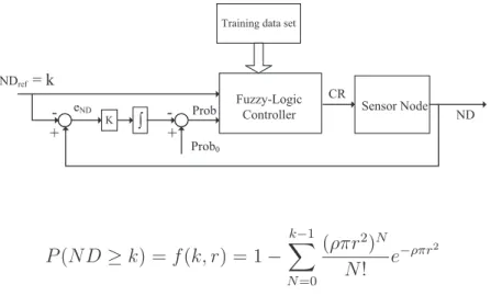
Figure 1 shows the system design of FTC. Adjusting the communication range (or equivalently transmission power) is a very common capability in many sensor nodes, e.g., Sun SPOT (Sun Small Programmable Object Technology) sensors. Hence, the output of FTC is the communication range (CR). Since the target is to reach a specific node degree (ND) for FTC, one of the inputs is the desired or reference ND, denoted by N Dref or k. Note that in this paper, we use N Dref and k
interchangeably, becauseN Dref is used in control systems andk commonly represents the node degree
in the graph theory. On the other hand, for a large and random network, the number of nodes within its communication range is unknown. Nevertheless, according to the network deployment strategy, the probability that a node has node degree k is known. For a random and uniform deployment, the probability that the node degree is at least bigger than k is given by Equation (1) (see [9]), where r is the node communication range,nis the total number of nodes in the field, node densityρ= n
A, andAis
the area of the field. Therefore, the probability that a node has degreekis another fuzzy-logic controller input, denoted byP rob. In practice,kis an integer and communication range has an upper boundrmax,
so integerk >0and0≤r ≤rmax.
Figure 1.Fuzzy-logic topology control (FTC).
= k
P(N D ≥k) =f(k, r) = 1−
k−1
X
N=0 (ρπr2
)N
N! e
−ρπr
2
3.1.2. FTC Learning Data Set
Provided a training data set from Equation (1), the fuzzy controller can be obtained through learning algorithms, such as neuro-adaptive learning algorithm. With the help of the Matlab “adaptive neuro-fuzzy inference system” (ANFIS) tool, FTC controller is not difficult to get. In ANFIS, the membership function parameters are automatically tuned through a backpropagation algorithm individually or in combination with a least square method. Once the data training is completed, the fuzzy inference system is available by simply using the function “evalfis” provided by Matlab. Hence, we concentrate on how to generate the training data set. As illustrated in Figure 1 and Equation (1), the inputs are N Dref and P rob, and the output is CR. Given ρ, N Dref ∈ {k1, k2,· · ·km} and
CR ∈ {r1, r2,· · ·, rj}, P rob = f(N Dref, CR) can be calculated from Equation (1). The training
data setT is as×3matrix in the form of [N Dref,P rob,CR], wheres =m·j. For instance, one item
in the training data set could be [3, 0.9, 25]. It means that the CR is set to 25m if the probability that
N Dref ≥3is 0.9.
3.1.3. P rob0 and K
SinceN Dref is characterized by the probability, it is necessary to adjust the node degree if a node
does not reachN Dref. For instance, ifCR = 25m can not lead to actualN D =N Dref, then next step
is to adjustP robto a higher value according to the node degree erroreN D. As shown in Figure1, there
is an integral controller outside the fuzzy control to adaptively change P rob. From the control theory point of view, the system properties (e.g., steady state) are controlled by parameterP rob0andK. IfeN D
is less than 0,K is configured to be half of its initial value. As a result,CRtends to increase faster than decrease. In Section4.2, we will further discuss the impact ofP rob0andKby simulation.
3.2. FTC Protocol
According to the design of FTC in Section 3.1, corresponding FTC protocol is presented in this section, as shown in FTC protocol running for a generic node. Each node broadcasts the HELLO message at the maximum communication range rmax, in order to collect neighbors’ information. The
communication range is modified accordingly based on the fuzzy-logic controller.
On the one hand, in this paper, we only consider undirected links (that is, there is a link between two nodes if and only if they are both in each other’s communication range), because in practice many routing protocols assume that the link between two nodes are undirected. On the other hand, FTC is a localized control algorithm running at each node independently. As a result, the node degree changes over time. For instance, nodeuis the neighbor ofv at this round of communication range updating, but it is likely that in next round uis not the neighbor of v due to the communication range of uand/orv
FTC protocol (for a generic nodei)
Require:
1: Training data set,T = [k,P rob,CR];
2: Maximum communication range,rmax;
3: Reference node degree,N Dref;
4: Initial Probability,P rob0;
5: InitialK,K0;
6: Number of rounds,rounds;
Ensure:
7: Obtain the fuzzy-logic control system by ANFIS, ANFIS(T);
8: CRi ⇐rmax;
9: P rob⇐P rob0;
10: whilerounds > 0do
11: Broadcast HELLO message with currentCRi;
12: For messages received from other nodes, store the ID of its neighbors;
13: Calculate the number of neighborsN Din the neighbor list;
14: CalculateeN D =N D−N Dref;
15: ifeN D <0then
16: K =K0;
17: else
18: K = K0
2 ;
19: end if
20: P rob⇐P rob−K ·eN D;
21: CRi ⇐evalf is(N Dref, P rob); %The outputCRican be calculated byCRi =evalf is(k, P rob)
22: rounds⇐rounds−1
23: end while
4. Simulation-Based Performance Evaluation
In this section, we evaluate our proposal FTC by using Matlab, comparing FTC with three representative localized topology control algorithms (FLSS, k-Neighbor, and LTRT), together with an algorithm without any control algorithms, called NONE in this paper. We will introduce them in Section4.3.
4.1. Preliminaries
FTC is applicable to a network when all nodes are randomly and uniformly deployed, because the training data derived from Equation (1) assumes that all nodes are randomly and uniformly deployed. However, FTC can be applied to other deployment strategies as long as the node degree distribution is able to be obtained. In our simulations, nodes are uniformly deployed at random in a 100×100 m2
field. All nodes are stationary after the deployment. The maximum communication ranges, denoted asrmax,
range within [0rmax]m. In this paper, we call one “round” simulation when all nodes finish the process
of executing a topology control algorithm one time. Recall thatnis the total number of nodes deployed in the field, andkis the desired node degree (namely,N Dref =k). In Section4.4, in order to simulate
different node densities, the number of nodes deployed in the area varies from 50 to 90 nodes. We randomly generate 50 networks for each specific number of nodes. For each network, we run different algorithms separately. The results are the average of 50 deployments.
4.2. Analysis of FTC Properties
As we mentioned in Section 3.1, FTC is affected by two parameters (P rob0 and K) outside the fuzzy-logic controller. The simulator provides average node degree calculated by the sum of node degree for all nodes divided by the number of nodes in the network. Figure2shows the impact ofKon network settling time, accuracy and stability. Firstly, the average node degree quickly converges to its steady state value (after about 10 rounds). Secondly, the average node degree converges to the reference node degree
k = 3. A lowerK results in a more stable system, but longer convergence time. For instance,K = 0.02 is more stable thanK = 0.1, butK = 0.02takes longer time to reach steady state. Thirdly, the system is stable, but the system demonstrates heavier oscillation behavior whenK is bigger.
Figure 2. Average node degree with different K (P rob0 = 0.8, n = 60, k = 3).
0 5 10 15 20 25 30
2.5 3 3.5 4 4.5 5 5.5 6
Node Degree
K = 0.02 K = 0.05 K = 0.08 K = 0.1
Rounds
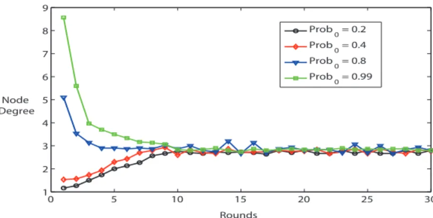
Figure 3. Average node degree with differentP rob0(K = 0.02, n = 60, k = 3).
0 5 10 15 20 25 30
1 2 3 4 5 6 7 8 9
Node Degree
Prob
0 = 0.2
Prob
0 = 0.4
Prob0 = 0.8
Prob0 = 0.99
Figure3illustrates different features at the first several rounds. IfP rob0is higher at the beginning, the nodes are more likely to be connected than P rob0is lower. Nevertheless, the average node degree goes to stable state after 10 rounds as well. As a result,P rob0has an impact on the initial status of network.
In short, the simulation results illustrate that K has an important influence on network settling time, accuracy and stability. In the following simulations, we choose K = 0.02, P rob0 = 0.8 and
rounds= 15to configure the parameters described in FTC protocol.
4.3. NONE, FLSS, k-Neighbor, LTRT
In this section, we briefly introduce four algorithms we have compared FTC with. More details can be found in the corresponding references.
• NONE: once all sensor nodes are deployed in the field, each node configures its communication range to the maximum communication range, and the communication range does not change during the simulation. NONE generates the most connected network, thus gives the upper bound of network connectivity. NONE algorithm is used to simulate the case that there is no topology control applied to WSNs.
• Fault-tolerant Local Spanning Subgraph (FLSS) [2]: each node runs at their maximum communication range to collect neighbors’ information, e.g., IDs, locations. Based on this information, each node first sorts all edges in an ascending order, and then only selects edges according to the order if it is notk −connectedto it. Maybe some edges are directed, but it is optional to only consider bi-directional edges by deleting directed edges, or turning directed edges into bi-directional edges.
• k-Neighbor algorithm [10]: each node first runs at its maximum communication range as well, in order to collect neighbor IDs and location information. Its final communication range is set to the distance between itself and itsk−thnearest neighbor. One of the important features of k-Neighbor is that the algorithm is asynchronous. Each node starts running its topology algorithm at a random time. However, the difference between nodes wake up is bounded by a known constant∆. By the time4∆+2d+τ, all nodes terminate setting the communication range, wheredis the time to obtain a specific contention free wireless with probability P, andτ is the upper bound of processing time for sorting neighbors. In the circumstances that the number of neighbors is less thank, k-Neighbor algorithm modifies its communication range to the distance to the farthest neighbor.
• Local Minimum Spanning Tree (LTRT) [3]: LTRT performs local spanning tree algorithmktimes. Given a networkG(V, E), whereV is the set of nodes,E is the set of links. LTRT calculates one of its spanning treesT(V,Eˆ1), and then removes all links inEˆ1 fromE. The resulting network is denoted asG(V, E−Eˆ1). Next, the same process is conducted onG(V, E−Eˆ1). Afterktimes, the final network is formed by combining all trees together, that isG(V,Eˆ1+ ˆE2+· · ·+ ˆEk). The
final communication range of each node is the maximum communication range inG(V,Eˆ1+ ˆE2+ · · ·+ ˆEk).
bek−connectedif the original network is at leastk−connected. On the contrary, k-Neighbor algorithm only proves that the network is1−connected with high probability ifk is the order ofΘ(logn). Like FLSS, k-Neighbor and LTRT, FTC proposed in this paper is also a fully localized algorithm to find k
neighbors, but FTC does not need location information. Similar to k-Neighbor, FTC cannot guarantee that the network is 100% connected either, but FTC can achieve the desired k, and therefore FTC can make the network connected with high probability if choosingkappropriately.
4.4. Comparison and Discussion
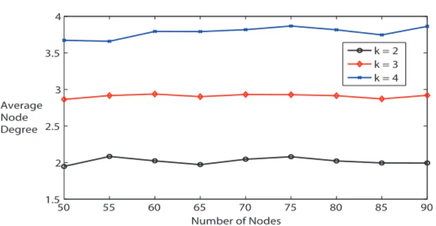
First, we evaluate whether FTC is able to trace theN Dref ork. As illustrated in Figure4, the average
node degree is very close to the desired node degree whenk = 2as the number of nodes varies from 50 to 90. Whenkis bigger, the average node degree is slightly lower than expected, because it is less likely to get more neighbors. For instance, with the same communication range, the probability of having 4 neighbors is obviously lower than having only 2 neighbors. In addition, the maximum communication range is limited. We can conclude from Figure4that FTC is able to achieve desired average node degree
k without knowing the locations of neighbors. Later, we will show that only k-Neighbor algorithm can achieve desired node degree as FTC, but k-Neighbor requires location information of neighbors.
Figure 4. Different desired node degree k.
50 55 60 65 70 75 80 85 90
1.5 2 2.5 3 3.5 4
k = 2 k = 3 k = 4
Number of Nodes Average
Node Degree
Figure 5. Example of resultant topology (n = 65, k = 3). (a) NONE; (b) k-Neighbor; (c) FLSS; (d) LTRT; (e) FTC.
0 20 40 60 80 100
0 20 40 60 80 100 1 2 3 4 5 6 7 8 9 10 11 12 13 14 15 16 17 18 19 20 21 22 23 24 25 26 27 28 29 30 31 32 33 34 35 36 37 38 39 40 41 42 43 44 45 46 47 48 49 50 51 52 53 54 55 56 57 58 59 60 61 62 63 64 65
(a)
0 20 40 60 80 100
0 20 40 60 80 100
1 2
3 4
5
6
7 8
9 10 11 12 13 14 15 16 17 18 19 20 21 22 23 24 25 26 27 28 29 30 31 32 33 34 35 36 37 38 39 40 41 42 43 44 45 46 47 48 49 50 51 52 53 54 55 56 57 58 59 60 61 62 63 64 65
(b)
0 20 40 60 80 100
0 20 40 60 80 100
1 2
3 4
5
6
7 8
9 10 11 12 13 14 15 16 17 18 19 20 21 22 23 24 25 26 27 28 29 30 31 32 33 34 35 36 37 38 39 40 41 42 43 44 45 46 47 48 49 50 51 52 53 54 55 56 57 58 59 60 61 62 63 64 65
(c)
0 20 40 60 80 100 0 20 40 60 80 100
1 2
3 4
5
6
7 8
9 10 11 12 13 14 15 16 17 18 19 20 21 22 23 24 25 26 27 28 29 30 31 32 33 34 35 36 37 38 39 40 41 42 43 44 45 46 47 48 49 50 51 52 53 54 55 56 57 58 59 60 61 62 63 64 65
(d)
0 20 40 60 80 100 0 20 40 60 80 100 1 2 3 4 5 6
7 8
9 10 11 12 13 14 15 16 17 18 19 20 21 22 23 24 25 26 27 28 29 30 31 32 33 34 35 36 37 38 39 40 41 42 43 44 45 46 47 48 49 50 51 52 53 54 55 56 57 58 59 60 61 62 63 64 65
(e)
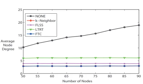
calculates where the k−th nearest neighbor is, based on already known distance information. FTC, on the contrary, is able to reach the desired k (see also Figure 4), but without knowing the neighbor locations. LTRT’s node degree is the second higher. As shown in previous Figure 5d, LTRT shows its superiority over FTC, FLSS, and k-Neighbors concerning the network connectivity.
Figure 6. Average node degree (k = 3).
50 55 60 65 70 75 80 85 90 0
5 10 15 20 25
Average Node Degree
NONE k−Neighbor FLSS LTRT FTC
Number of Nodes
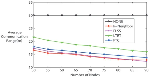
Moreover, it is worth noting that the communication range is proportional to the energy consumption of wireless sensor nodes. Therefore, a lower average communication range implies a lower energy consumption, which is a significant performance when designing WSNs. Figure 7shows the average communication range. Recall that the maximum communication range of each node is 30 m in the simulation. On the one hand, apart from NONE algorithm (because the communication range of each node is fixed at maximum), other algorithms’ average communication range decreases along with the number of nodes in the network increasing, because higher node density indicates that it is more likely to have the desired node degree with lower communication range. With the number of hops increasing, the energy consumption due to wireless transmission decreases, but the energy consumption due to forwarding messages increases. Overall, though, the energy is still saved, because the energy spent on wireless transmission is orders of magnitude higher than that spent on computation. So, we can conclude that energy consumption is lower if the node density is high for all algorithms (except NONE). On the other hand, from Figure7, it can be seen that in terms of energy consumption, NONE is the worst, and LTRT is the second worst. FTC, FLSS and k-Neighbors performance is very close to each other, but it is better than NONE and LTRT.
Finally, Figure 8 demonstrates the average maximum communication range. FTC maintains the lowest maximum communication range comparing it with other algorithms, which means that the most energy-consuming node in the network consumes the lowest power. Furthermore, Figure9evaluates the Energy Expended Ratio (EER) (defineEER = 100× CRavg
Figure 7.Average communication range (k = 3).
50 55 60 65 70 75 80 85 90 10
15 20 25 30 35
Average Communication
Range(m)
NONE k−Neighbor FLSS LTRT FTC
Number of Nodes
Figure 8. Average maximum communication range (k = 3).
50 55 60 65 70 75 80 85 90
10 15 20 25 30 35
Maximum Communication
Range(m) NONE
k−Neighbor FLSS LTRT FTC
Number of Nodes
Figure 9.Energy expended ratio (EER) (k = 3).
50 55 60 65 70 75 80 85 90
40 50 60 70 80 90 100 110
EER
NONE k−Neighbor FLSS LTRT FTC
Number of Nodes
5. Conclusions and Future Works
number of one-hop neighbors a node has), therefore in turn improving the network connectivity. Unlike other ways to design fuzzy-logic control system, the fuzzy-logic controller of FTC is constructed from a training data set. One of the great advantages of this approach is that it is easier to design a feasible controller without complicated parameter adjustment for the fuzzy-logic controller, especially when the network is highly dynamic.
FTC has been compared with four representative localized algorithms: NONE, FLSS, k-neighbors and LTRT. The simulation results show that FTC is able to trace the desired node degree as k-Neighbor algorithm which is based on the locations of neighbors, but FTC does not depend on location information. On the contrary, NONE, FLSS, and LTRT are unable to achieve the desired node degree. The average communicating range of FTC is very close to FLSS and k-Neighbor, but lower than NONE and LTRT. It implies that the energy consumption of FTC is lower than that of NONE and LTRT. In addition, the average maximum communication of FTC is the lowest, which means that the highest energy-consuming node in the network running FTC protocol consumes the lowest power than running other algorithms. The Energy Expended Ratio (EER) of FTC is very close to LTRT, but higher than FLSS and k-Neighbor. In summary, without knowing the neighbor location information, our localized FTC shows the capability of achieving desired node degree, maintaining network connectivity, and it is energy-efficient.
In this paper, all nodes are stationary after they are deployed. In our future works, we will take into account the mobility of sensor nodes. Furthermore, our validations are based on computer simulations. In order to validate FTC protocol, real experiments will be carried out on our Sun SPOT sensor platform in the near future. The node deployment is very unlikely to be an ideal random and uniform distribution, so we will calculate all sensor nodes’ locations through computer simulation prior to deploying them in the field.
Acknowledgments
This work is supported by the European project “Design, Monitoring and Operation of Adaptive Networked Embedded Systems” (DEMANES) (project code ARTEMIS-JU:295372) and Spanish “Ministerio de Industria, Energ´ıa y Turismo” (project code ART-010000-2012-2).
Author Contributions
Yuanjiang Huang, Jos´e-Fern´an Mart´ınez and Juana Sendra were responsible for the theoretical analysis of the control system. Yuanjiang Huang, Jos´e-Fern´an Mart´ınez and Vicente Hern´andez designed the simulation procedure and analyzed the simulation results. The simulation platform is being developed by the Research Group of Next-Generation Networks and Services (GRyS), where the authors belong to.
Conflicts of Interest
References
1. Balister, P.; Sarkar, A.; Bollob´as, B. Percolation, Connectivity, Coverage and Colouring of Random Geometric Graphs. InBolyai Society Mathematical Studies; Springer: Berlin/Heidelberg, Germany, 2008; Volume 18, pp. 117–142.
2. Li, N.; Hou, J. Localized fault-tolerant topology control in wireless ad hoc networks. IEEE Trans. Parallel Distrib. Syst. 2006, 17, 307–320.
3. Miyao, K.; Nakayama, H.; Ansari, N.; Kato, N. LTRT: An efficient and reliable topology control algorithm for ad-hoc networks. IEEE Trans. Wirel. Commun. 2009, 8, 6050–6058.
4. Kulkarni, R.; Forster, A.; Venayagamoorthy, G. Computational Intelligence in Wireless Sensor Networks: A Survey. IEEE Commun. Surv. Tutor. 2011, 13, 68–96.
5. Feng, G. A Survey on Analysis and Design of Model-Based Fuzzy Control Systems. IEEE Trans. Fuzzy Syst. 2006, 14, 676–697.
6. Bagci, H.; Yazici, A. An energy aware fuzzy approach to unequal clustering in wireless sensor networks. Appl. Soft Comput.2013, 13, 1741–1749.
7. Costa, P.; Cesana, M.; Brambilla, S.; Casartelli, L. A cooperative approach for topology control in Wireless Sensor Networks. Pervasive Mob. Comput.2009, 5, 526–541.
8. Guo, L.; Xu, H.; Harfoush, K. The Node Degree for Wireless Ad Hoc Networks in Shadow Fading Environments. In Proceedings of the 2011 6th IEEE Conference on Industrial Electronics and Applications (ICIEA), Beijing, China, 21–23 June 2011; pp. 815–820.
9. Bettstetter, C. On the Minimum Node Degree and Connectivity of a Wireless Multihop Network. In MobiHoc ’02 Proceedings of the 3rd ACM International Symposium on Mobile ad Hoc Networking & Computing; ACM: New York, NY, USA, 2002; pp. 80–91.
10. Blough, D.; Leoncini, M.; Resta, G.; Santi, P. The k-Neighbors Approach to Interference Bounded and Symmetric Topology Control in Ad Hoc Networks. IEEE Trans. Mob. Comput. 2006, 5, 1267–1282.
11. Aziz, A.; Sekercioglu, Y.; Fitzpatrick, P.; Ivanovich, M. A Survey on Distributed Topology Control Techniques for Extending the Lifetime of Battery Powered Wireless Sensor Networks. IEEE Commun. Surv. Tutor. 2013, 15, 121–144.
12. Zhu, C.; Zheng, C.; Shu, L.; Han, G. A survey on coverage and connectivity issues in wireless sensor networks. J. Netw. Comput. Appl. 2012, 35, 619–632.
13. Younis, M.; Senturk, I.F.; Akkaya, K.; Lee, S.; Senel, F. Topology management techniques for tolerating node failures in wireless sensor networks: A survey. Comput. Netw. 2013,58, 254–283.
14. Wang, B. Coverage Problems in Sensor Networks: A Survey. ACM Comput. Surv. (CSUR)2011, 43, 32:1–32:53.
15. Bondy, A.; Murty, U. Graph Theory; Springer: Berlin/Heidelberg, Germany, 2008.
16. Guerriero, F.; Violi, A.; Natalizio, E.; Loscri, V.; Costanzo, C. Modelling and solving optimal placement problems in wireless sensor networks. Appl. Math. Modell. 2011, 35, 230–241.
18. Asorey-Cacheda, R.; Garc´ıa-S´anchez, A.J.; Garc´ıa-S´anchez, F.; Garc´ıa-Haro, J.; Gonz´alez-Castano, F.J. On Maximizing the Lifetime of Wireless Sensor Networks by Optimally Assigning Energy Supplies. Sensors2013, 13, 10219–10244.
19. Byrka, J.; Grandoni, F.; Rothvoß, T.; Sanit´a, L. An Improved LP-based Approximation for Steiner Tree. In Proceedings of the 42nd ACM Symposium on Theory of Computing; ACM: New York, NY, USA, 2010; STOC ’10, pp. 583–592.
20. Senel, F.; Younis, M. Relay node placement in structurally damaged wireless sensor networks via triangular steiner tree approximation. Comput. Commun.2011, 34, 1932–1941.
21. Alfadhly, A.; Baroudi, U.; Younis, M. An Effective Approach for Tolerating Simultaneous Failures in Wireless Sensor and Actor Networks. In Proceedings of the First ACM International Workshop on Mission-oriented Wireless Sensor Networking; ACM: New York, NY, USA, 2012; MiSeNet ’12, pp. 21–26.
22. Lee, S.; Younis, M. Recovery from multiple simultaneous failures in wireless sensor networks using minimum Steiner tree. J. Parallel Distrib. Comput. 2010, 70, 525–536.
23. Degener, B.; Fekete, S.P.; Kempkes, B.; auf der Heide, F.M. A survey on relay placement with runtime and approximation guarantees. Comput. Sci. Rev.2011, 5, 57–68.
24. Brito, M.; Ch´avez, E.; Quiroz, A.; Yukich, J. Connectivity of the mutual k-nearest-neighbor graph in clustering and outlier detection. Stat. Probability Lett. 1997, 35, 33–42.
25. Xue, F.; Kumar, P.R. The Number of Neighbors Needed for Connectivity of Wireless Networks. Wirel. Netw. 2004, 10, 169–181.
26. Balister, P.; Bollob´as, B.; Sarkar, A.; Walters, M. Connectivity of random k-nearest-neighbour graphs. Adv. Appl. Probab.2005, 37, 1–24.
27. Yuanjiang, H.; Ortega, J.F.M.; Pons, J.S.; Santidri´an, L.L. The Influence of Communication Range on Connectivity for Resilient Wireless Sensor Networks Using a Probabilistic Approach. Int. J. Distrib. Sens. Netw. 2013, 2013, 1–11.
28. Hajiaghayi, M.T.; Immorlica, N.; Mirrokni, V.S. Power Optimization in Fault-tolerant Topology Control Algorithms for Wireless Multi-hop Networks. IEEE/ACM Trans. Netw. 2007, 15, 1345–1358.
29. Abellanas, M.; Garc´ıa, A.; Hurtado, F.; Tejel, J.; Urrutia, J. Augmenting the Connectivity of Geometric Graphs. Comput. Geom. Theory Appl. 2008, 40, 220–230.
30. Han, X.; Cao, X.; Lloyd, E.; Shen, C.C. Fault-Tolerant Relay Node Placement in Heterogeneous Wireless Sensor Networks. IEEE Trans. Mob. Comput. 2010, 9, 643–656.
31. Kashyap, A.; Khuller, S.; Shayman, M. Relay Placement for Higher Order Connectivity in Wireless Sensor Networks. In Proceedings of INFOCOM 2006 25th IEEE International Conference on Computer Communications, Barcelona, Spain, April 2006, pp. 1–12.
33. Bredin, J.L.; Demaine, E.D.; Hajiaghayi, M.; Rus, D. Deploying Sensor Networks with Guaranteed Capacity and Fault Tolerance. In Proceedings of the 6th ACM International Symposium on Mobile Ad Hoc Networking and Computing; ACM: New York, NY, USA, 2005; MobiHoc ’05, pp. 309–319.
34. Chen, B.; Jamieson, K.; Balakrishnan, H.; Morris, R. Span: An Energy-Efficient Coordination Algorithm for Topology Maintenance in Ad Hoc Wireless Networks. ACM Wirel. Netw. 2002, 8, 481–494.
35. Wang, X.; Xing, G.; Zhang, Y.; Lu, C.; Pless, R.; Gill, C. Integrated Coverage and Connectivity Configuration in Wireless Sensor Networks. In Proceedings of the 1st International Conference on Embedded Networked Sensor Systems; ACM: New York, NY, USA, 2003; SenSys ’03, pp. 28–39.
36. Ye, F.; Zhong, G.; Cheng, J.; Lu, S.; Zhang, L. PEAS: A Robust Energy Conserving Protocol for Long-lived Sensor Networks. In Proceedings of the 23rd International Conference on Distributed Computing Systems, Providence, RI, USA, 19–22 May 2003; pp. 28–37.
37. Fu, Y.; Sha, M.; Hackmann, G.; Lu, C. Practical Control of Transmission Power for Wireless Sensor Networks. In Proceedings of the 20th IEEE International Conference on Network Protocols (ICNP), Austin, TX, USA, 30 October–2 November 2012; pp. 1–10.
38. Lee, J.S.; Cheng, W.L. Fuzzy-Logic-Based Clustering Approach for Wireless Sensor Networks Using Energy Predication. IEEE Sens. J.2012, 12, 2891–2897.
39. Brante, G.; de Santi Peron, G.; Demo Souza, R.; Abrao, T. Distributed Fuzzy Logic-Based Relay Selection Algorithm for Cooperative Wireless Sensor Networks. IEEE Sens. J.2013, 13, 4375–4386.
40. Veena, K.N.; Kumar, B. Dynamic Clustering for Wireless Sensor Networks: A Neuro-Fuzzy Technique Approach. In Proceedings of the 2010 IEEE International Conference on Computational Intelligence and Computing Research (ICCIC), Coimbatore, India, 28–29 December 2010; pp. 1–6.
41. Ghataoura, D.S.; Yang, Y.; Matich, G. GAFO: Genetic Adaptive Fuzzy Hop Selection Scheme for Wireless Sensor Networks. In Proceedings of the 2009 International Conference on Wireless Communications and Mobile Computing: Connecting the World Wirelessly; ACM: New York, NY, USA, 2009; IWCMC ’09, pp. 376–380.
42. Budyal, V.; Manvi, S. ANFIS and agent based bandwidth and delay aware anycast routing in mobile ad hoc networks. J. Netw. Comput. Appl. 2014, 39, 140–151.
43. Ando, H.; Kulla, E.; Barolli, L.; Durresi, A.; Xhafa, F.; Koyama, A. A New Fuzzy-based Cluster-Head Selection System for WSNs. In Proceedings of the 2011 International Conference on Complex, Intelligent and Software Intensive Systems (CISIS), Seoul, Korea, 30 June–2 July 2011; pp. 432–437.
c