Joint 4-D variational stereo reconstruction and camera calibration refinement for oceanic sea state measurements

JOINT 4-D VARIATIONAL STEREO RECONSTRUCTION AND CAMERA

CALIBRATION REFINEMENT FOR OCEANIC SEA STATE MEASUREMENTS

Ping-Chang Shih Guillermo Gallego

Anthony Yezzi Francesco Fedele

INTRODUCTION

ABSTRACT

Validating modern oceanographic theories using models produced through stereo computer vision principles has recently emerged. Space-time (4-D) models of the ocean surface may be generated by stacking a series of 3-D reconstructions indepen-dently generated for each time instant or, in a more robust man-ner, by simultaneously processing several snapshots coherently in a true "4-D reconstruction." However, the accuracy of these computer-vision-generated models is subject to the estimations of camera parameters, which may be corrupted under the influ-ence of natural factors such as wind and vibrations. Therefore, removing the unpredictable errors of the camera parameters is necessary for an accurate reconstruction. In this paper, we pro-pose a novel algorithm that can jointly perform a 4-D reconstruc-tion as well as correct the camera parameter errors introduced by external factors. The technique is founded upon variational optimization methods to benefit from their numerous advantages: continuity of the estimated surface in space and time, robustness, and accuracy. The performance of the proposed algorithm is tested using synthetic data produced through computer graphics techniques, based on which the errors of the camera parameters arising from natural factors can be simulated.

Within the past twenty years, computer vision principles have been gradually adopted to create three-dimensional (3-D) models of the ocean surface for measurement and analysis pur-poses. These computer models are generated through a process known as 3-D reconstruction in the field of stereo computer vi-sion, where the 3-D shape of an object is recovered based on its 2-D projections (e.g. observed images) obtained from various viewpoints.

Variational 3-D reconstruction methods have been founded upon the advantages of the calculus of variations to overcome the aforementioned disadvantages of feature-based methods. By converting a computer vision problem into a variational opti-mization one, these 3-D reconstruction methods approximate the surface of the target object by piece-wise smooth functions [8,9] instead of a collection of 3-D points. Therefore, users can ar-bitrarily sample the functions to visualize the model at any res-olution or to analyze the model at any location. Utilizing this concept, Gallego et al. [10-12] proposed a variational frame-work to reconstruct the space-time model of a patch of ocean surface. In this framework, the reconstructed surface of the ob-ject is obtained as the minimizer of a functional that takes into account both the smoothness of the surface and its photomet-ric error. The latter quantifies the discrepancy between the mea-surements (snapshots of videos) and the "reprojections" of the reconstruction onto measurements via mathematical coordinate transformations and pin-hole projection formulas. The resulting reconstruction consists of two parts: the height or elevation map and the superficial texture pattern (called radiance map) of the ocean surface. When the radiance map is superimposed on top of the elevation map, a computer model of the ocean surface is obtained.

However, the accuracy of all aforementioned computer-vision-generated models strongly depends on the accuracy in the determination of the cameras' parameters, a technique called camera calibration. These parameters specify the perspective projection operation carried out by the cameras (mapping points in the 3-D world to 2-D sensors) and its inverse operation (back-projection), hence they have a direct effect in the evaluation of reprojection errors. The reconstruction process is very sensitive to the changes of camera parameters, e.g., small deviations of the camera parameters can cause a magnified incorrect repro-jection error and, consequently, change the minimizers of the error functional, yielding incorrect reconstruction. Since cam-eras are installed outdoors in real applications, extrinsic camera parameters—parameters that accounts for the relative orientation and location of the cameras in the scene—are prone to be per-turbed by natural factors such as breeze or vibrations. Therefore, the reconstruction of a patch of the ocean surface over a time in-terval should not be performed alone but be incorporated with a camera calibration refinement technique.

In this paper, we address the problem of reconstructing a patch of the ocean surface over a given period of time in the case that the extrinsic camera parameters might be perturbed by environmental factors. To this end, we adopt a variational opti-mization framework and jointly estimate the 4-D reconstruction of the ocean surface and the refinement of the camera param-eters as the minimizers of an error functional that measures /) the photometric error between acquired videos and the reprojec-tion of the 4-D reconstrucreprojec-tion onto the videos, ii) the spatial and temporal smoothness of the reconstruction, and Hi) the temporal

variance of the perturbed camera parameters. As a result of itera-tively obtaining the minimizers of the error functional, our algo-rithm can reconstruct the space-time model for the target region and decrease the influence of the errors caused by deviations of the camera parameters on the reconstruction. Since introducing the desired perturbations to the camera parameters and acquiring the ground truth of the reconstruction in real cases are difficult tasks, we validate the algorithm and show its effectiveness by applying it to reconstruct a synthetic ocean surface generated by a computer graphics tool (OpenGL) under the conditions that de-viations are deliberately added into the true camera parameters.

METHODOLOGY

Notation and Geometric Image Formation

We use XT to denote the coordinates of a general point on the model observed in the world coordinate system at moment T. When observed by the i01 camera coordinate system, XT can be

expressed as X¡ = (X;,Y;,Z;)T. Coordinates XT and X¡ are lin-early related by a rigid body motion, X; = R JXT+1], where R] is

a three-by-three rotation matrix accounting for the difference be-tween the orientations of the world and the i01 camera coordinate

systems, and t] e R3 is the displacement between the origins of the two systems.

Suppose the apertures of the cameras are small enough and lens are ideal. Thus, the imaging of a 3-D point onto the sensor can be approximated as a pin-hole model without considering the distortion effects of lens; as such, each point X¡ is projected onto a 2-D point x on the image plane using the pin-hole projection formula: x = (xj)J = (X¡/2¡, Y¡/2¡)T.

Up to now, x is given with respect to the ith camera

coordi-nate system, so one more transformation is required to convert it to pixel coordinates x = (x,y)T, i.e., the position of x on a CCD

image plane. Such a transformation is given by

x =

where the internal parameters of the camera (L'x and L'y are the

focal lengths and (x'0,y'0) is the principal point of the ith camera,

in pixel units) are compactly represented by the intrinsic camera matrix [13]

K,- =

Note that we use bold fonts to represent vector quantities and add superscript T to the extrinsic parameters of the cameras —RJ and t]—to emphasize their temporal dependence due to

X y_ =

"4 o"

_° 4.

+

x0

A

"4

0

V

0 x0

fo

Xi

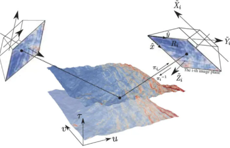
FIGURE 1: Illustration of the space-time reconstruction of a

patch of ocean surface. The synchronized cameras film the same area for a period of time while the extrinsic camera parameters may be perturbed by environmental factors. The stacked graphs in the middle symbolize the ocean surface at different moments in time. Each point on the space-time reconstruction is repre-sented as XT, which is imaged by the cameras and then converted

to pixel coordinates x.

the possible influence of environmental factors, whereas such a notation is not used in case of the intrinsic camera parameters in K; since we assume that they remain constant or that the effect on the system of their small variations is negligible compared to that of the extrinsic parameters. In addition, to simplify notation, T is not particularly used on some symbols such as x, x, and X;, even though they are time dependent. All symbols and their relationships are geometrically shown in Fig. 1.

Proposed Error Functional

To jointly reconstruct a dense space-time model of a patch of ocean surface and simultaneously refine the extrinsic camera parameters, we propose the following error functional

E ( / , Z , A ) = W / , Z , A ) ( 1 )

"T ^geom (ZJ + iirad \J ) ~r ^cam \" ) .

In this functional, Z and / are functions of three variables (w, v, T) with domain in Uj := U x [0,7], where u = (w,v)T £ U are

spatial variables and T G [0, T] is the temporal variable (as il-lustrated in Fig. 1). From the visual perspective, Z(W,V,T) and /(W,V,T) represent the shape and the texture of the model on parameter point (w,v) at time T (as shown in Fig. 2), respec-tively, so XT = (w,v,Z(w,v,T))T. The vector function A(T) =

(A1 (T), ..., Xm(z))T denotes the extrinsic camera parameters

es-timated within the observation interval of duration T. The

func-FIGURE 2: Relationship between the elevation map (Z), the

ra-diance map (/), and the reconstructed surface for a given time T. The reconstructed surface is formed when each spatial coordinate Z(w, v, T) is tinted with "color" or intensity value /(w, v, T).

tion AJ represents a single camera parameter. The minimizers of

this functional—a special set of (/,Z, A)—are expected to opti-mally fit the visual measurements and appropriately approximate the superficial properties on the observed ocean surface and the temporal variations of the camera parameters. Therefore, £data>

EgQom, £rad> and Ecam are designed as follows:

£data = [ t [ I (//(x) -f(7ir\x))fdxd^ (2)

JTÍ=IJRÍ Z

£geom = \ J J (Z¡ + Zv2 + Z?) dVL d*C, (3)

£rad = | J J {fl+fi+fi) dudT, (4)

2 JT JT-W 2W

where a, j8,7 > 0. In the data fidelity term ((2)), Nc is the

num-ber of cameras, Ri is the reprojection region of the reconstruc-tion at time x on the /th image (denoted by //), and //(x) is the

image intensity at pixel x. The forward perspective projection (the aforementioned coordinate transformations from XT to x in

the previous section) is represented by 7%, and, by abuse of no-tation, its inverse operation is represented by %^x. In the

for-mulation, the first term of ¿data ((2)) quantifies the sum of the discrepancies between the measurements (the acquired synchro-nized stereo videos) and the reprojections of the reconstructed surface onto the image planes.

Because the target object is the ocean surface, the shape (Z) and the texture (/) can be assumed to be smooth functions with respect to time and space, which is formulated in (3) and (4). The term £ge0m measures the spatial and temporal smoothness

same for / .

Given that natural factors such as breeze or vibrations smoothly influence the extrinsic camera parameters, we design ^cam to restrict the temporal behavior of X. Instead of penaliz-ing the temporal changes of X in terms of derivatives, as it is done with Z and / in (3) and (4), £c a m is designed to penalize the temporal variations of X with respect to a local variance, as expressed by (5). In the equation, ¡i{x;w) represents the local mean of X in an interval of duration 2w centered around time T. that is,

H{x;w) = 1

2w z+w

X(q)dq. (6)

By choosing an appropriate w, we can eliminate different types of perturbations on the camera parameters that are otherwise not possible to be removed using penalties on the derivatives.

Minimizers of the Error Functional The minimizers

of (1) are determined by the zero functional derivatives with

re-8E 8E 8E

spect to the arguments (denoted by | § = 0, | y = 0, and ff = 0,

Mj = 0 for all j). Methods for deriving the analytical forms

i.e.,

of I f and I f are explored in [12]. Although the error functional _{sz Sf} in [12] differs from (1), | | = 0 and | f = 0 yield the same set of partial differential equations (PDEs),

g(ZJ) - aAZ = 0 in UT,

Nc

•^(Ii-m-P^f = 0 in UT,

i = i

r\7

b(ZJ) + a-j- = 0 on dUT:

B^J- =QondUT -dv

(7)

(8)

(9)

(10)

In the equations above, g(Z,f) and b(Z,f) are nonlinear terms due to the data fidelity component of the error functional,

g(Z,f)=V{UiV)f-Y,\Ki\Z^(Ii-f)(u-CJ,v-Ci

h

Nc

b(Z,f) = ld-(I¡-f)2\K¡\Z7\(u-C¡)vu + (v-q -2)vv)

(=1

and /,- is the Jacobian of the change of variables from U to the ith

image plane, i.e., J¡ = |K¡|Zr3 max (0, - ( XT - C¡, X* x XJ}) ac-cording to the derivations in [11]. The symbol d in (9) and (10) has two different and standard meanings: it represents the direc-tional derivative operator, as in | | , or indicates the boundary of the domain of Z and / , as in dllr- Finally, V = (v", vv, vT)T is

the unit outward normal on dUj, and C¡ = (C¡,Cf,Cf) l is a

vector with the world coordinates of the i01 camera center.

To compute | £ , we augment X with an artificial time vari-able t and differentiate X with respect to t using chain rule rela-tionship, yielding ¿f = (j§J^tJ)L , where (v)L2( r ) is the

L2 -inner product operator between functions defined over the in-terval of duration T. This lays down the path toward obtaining an extrema of E by evolving X with respect to t using a descent method.

Thus, differentiating E with respect to t leads to

dE ~dt

dE, data dEc,

dt dt (11)

where the smoothness terms in £geom and Eiad vanish because

they do not depend on the camera parameters X. Next, let us show how to compute each term in (11), starting with the data fidelity one: Since R] and t] are the parameters of the ith camera,

we can drop the summation symbol in (2) when differentiating E with respect to t. Hence,

dE, data

dt T dt ^jR\{li{t)-f{n.l(t))fd^dz. (12)

Operator j j in (12) cannot be directly moved inside JR. because Ri depends on Xi, and consequently on t. In this case, deriving

the analytical form of (12) requires the use of Reynolds' trans-port theorem and a change of variables, which was completed by Shih et al. in [14]. Compared with the assumption in this paper, the extrinsic camera parameters discussed in [14] are regarded as temporally constant variables, which, nevertheless, does not af-fect the reasoning process of the derivations in this case. Hence, the right hand side of (12) is ultimately differentiated as

3-Edata

dt V:

, [ii(x,(xz))-f(xzJ\2 ¿MX*)) ^ ¿ N x * ) )X j

+ [ [ / ( Xt) - /j( ai( Xt) ) ] < ^)Vi/ ( Xt) ) J 'jd « \ ,

JU I L2(T)

(13)

where (•, •} is the usual inner product operator in R" ((a,b) =

aJb) and Q is a planar (two-by-two) rotation matrix that rotates

a unit tangent vector to the corresponding outward normal. In addition, Vs/ stands for ( ^ - ) , which is (/„, fv, 0)T.

3{*i(Xz))

dli and

With different types of camera parameters,

j in (13) possess different analytical forms. For example, if

'Although C; = —(R?)Tt? depends on T, the corresponding superscript is not

X = t], according to [14],

dX

UXZ^ 0 - Z ¿ X¡ Y . 7 - 2 fZ :

¡ 7 - 1 _ r ! ' v . 7 - 2 0 Z > Z r ' - Z < YfZ :

and

~Jx

T N - l

I d 3 x 3 X.-N,-1

X7N;

where N¡ is an outward normal on the reconstructed model ob-served in the ft1 camera frame. Furthermore, [14] indicates that

if X = a>¡ (a>¡ is the rotation vector of R] in exponential coordi-nates), then

¿fc(X

))

dX

0 - 4 X;Z r2 0 Z^Zr1 - Z ^ Z r2

¿izr

and

<9XT

(R?

I d 3 x 3 • R?[X*

Next, let us deal with the second term in (11). Taking into account that X = X{p,t) depends on t, and therefore ¡l =

IÜ(T,Í;W) mdEcam(X) depend on t, too, the second term in (11)

is computed as follows:

dEc, dt

r rZ+w -\

¿ y j ^ ^ (X-n)

^(X-n)dpdx.

Because \lt does not depend on p, \it can be moved out of the

inner integral. As such,

z+w

{X-n)Jiitdp = z+w

{X-n)dp) ¡it = 0,

H{x) = 1 i f x > 0

0 otherwise

which accounts for the fact that the integrand of (14) may not vanish if T - w < p < t + w, or equivalently, if p — w <t <p + w

. Then, recalling that X = X{p,t) and n = ¡i{x,t;w) in (14), it

becomes

dE, _cam

¿ J y Xj(X-ii)W(T,p;w)dTdp

i y_ f

2w JT i y_ fp+w

2w

-JT1

J I \ ^'r J p — W 0-^cam

(X -n)W(T,p;w)dT ) dp

(X-p)d%

= (Xt

sx

using the vectorial version of (•, -)L2iT\ • Therefore, we identify

SX

,

«=¿£>-''>

= Y[X(P) 2w

rp+w

2w X(q)dq d%

where in the last line we substituted the definition (6) for the local mean \i and omitted the dependence of X with respect to t.

Combining the functional gradients (with respect to the cam-era parameters) of the data fidelity and the camcam-era refinement components of the error functional, the gradient descent flow cor-responding to | £ = 0 is Xt = - f f • Therefore,

x>

=-\L ['•

-

'

,'

'

'']

^ga,

^gi)„

IdU dXJ ds

[/(XT) -/f(jn-(XT))] < | ^ , VS/ ( XT) ) ^

+yX] {%)-4w2

rz+w

X]{q)dq )dz\, V/. (16)

so we are left with

<5£cam 7 r rZ+w

dt 2w JT JT_W (X-tl)JXtdpdx. (14)

To further simplify (14), let us swap the order of integration by using a window function W(T, p; w) = H{p — t + w) H{p

-t - w). H is -the Heaviside s-tep func-tion defined as

is the cross product matrix associated to

0 — <Z3 ú¡2

2Matrix [a] x = a-¡ 0 —a\

—ai a\ 0

vector a = (a\, 02, «23 )T £ R3 so that a x b = [a] x b for all b e R3.

EXPERIMENTS

Synthetic Data

Computer graphics and 3-D reconstruction applications are reverse operations of each other. In computer graphics, imagi-nary objects are created in a virtual world and can be viewed from various angles. Using computer graphics tools, such as OpenGL, we can create a region of deforming ocean waves in a virtual world and set up multiple virtual cameras to acquire videos of the synthetic ocean surface. The synthetic ocean waves will be a dense 3-D point cloud deforming with respect to time in which the coordinates (in the virtual world) of all points are known (because we create them), and textures will be rendered on the point cloud as the superficial pattern of the synthetic waves. The videos—the contents shown in the application programming in-terface (API) windows—can be read from the memory of the computer graphics card. However, because the reference frame of the virtual world is different from that of our algorithm, we must perform a coordinate transformation (a rigid body motion) to express the simulated extrinsic camera parameters in the ref-erence system used by the algorithm. After this information is ready, we can add errors to the camera parameters, reconstruct the model of the synthetic waves, and apply our calibration re-finement algorithm to see how the reconstruction is rectified. By deliberately discretizing the elevation and radiance maps of the reconstructed model with the same number of samples as the in-put point cloud, we can verify the accuracy of the reconstructed model by point-wise comparison with respect to the input point cloud and radiance.

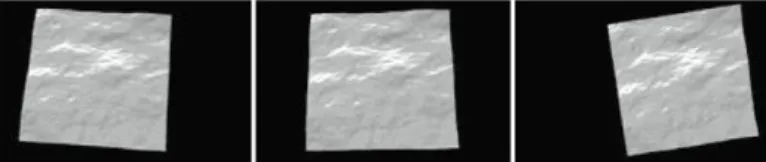
The configuration of the synthetic data is illustrated in Fig. 3. A deforming ocean surface is created in a virtual world and ob-served from three different positions (as shown in Fig. 3a) for a specified time interval. Artificial errors are added to the true extrinsic camera parameters converted from the configuration of virtual scene developed using OpenGL. Since the purpose of this experiment is to explore the performance of our algorithm un-der the smooth influence of environmental factors, the artificial errors are deliberately smoothed within the observation interval (nine temporal samples), as shown in Figs. 3b and 3c.

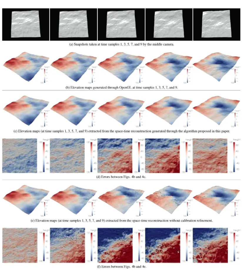
We particularly take out the inputs and outputs at temporal samples 1, 3, 5, 7, and 9 for demonstration. The visual observa-tions of the deforming ocean surface are listed in Fig. 4a, and the elevation maps produced through OpenGL at those time samples are listed in Fig. 4b. The width and height of the surface are set to be 7,475.2 mm, and the range of the height is configured to be

[-500,450] mm, as marked by the hue bars.

We initially set a = 5, /3 = 50, y = 500, and w = 3 for nu-merically solving (7) - (10) and (16). These parameters pro-duce a rough reconstruction. Afterward, we continue to solve the aforementioned equations while a, ¡5,y, and w are gradually reduced to a = 0.2, /3 = 0.025, y = 100, and w = 1. Eventually, the elevation maps generated through this process are shown in Fig 4c. In addition, the differences between Figs. 4b and 4c are shown in Fig. 4d. All hue bars are given in millimeter units.

•DC

(b) Errors introduced to the translational part t¡ of the extrinsic parameters.

(c) Errors introduced to the rotational part R¡ of the extrinsic parameters.

FIGURE 3: Configuration of the synthetic data: Artificial errors,

temporally smooth, are added to corrupt the true camera param-eters converted from OpenGL to simulate the effects imposed by natural factors on a 3-D reconstruction camera system. Note that the vertical axes indicate that errors are limited to be less than 2% of the true values.

An experiment where the calibration refinement is not per-formed is conducted and shown in Fig. 4e for comparison. In this experiment, only (7)—(10) are solved; (16) is not used (i.e., 7 = 0 ) . The error maps between the outcomes of this experiment and the inputs are shown in Fig. 4f.

differ-(a) Snapshots taken at time samples 1, 3, 5, 7, and 9 by the middle camera.

J-

J

(b) Elevation maps generated through OpenGL at time samples 1, 3, 5, 7, and 9.

> i i i

(c) Elevation maps (at time samples 1,3,5,7, and 9) extracted from the space-time reconstraction generated through the algorithm proposed in this paper.

(d) Errors between Figs. 4b and 4c.

(e) Elevation maps (at time samples 1,3,5,7, and 9) extracted from the space-time reconstraction without calibration refinement.

h*oN

(f) Errors between Figs. 4b and 4e.

enees. In addition, the effect of the calibration refinement can be observed from the comparison between Figs. 4d and 4f.

In the case in which the reconstruction and the calibration refinement are jointly performed (as shown in Fig. 4d), most of the points in the error maps at time samples 1, 3, 5, 7, and 9 fall within the ±40 mm range. By contrast, when the reconstruction is executed without calibration refinement, a very large portion of the error maps exhibit colors beyond the range of the hue bars. Note that even /) with relatively large errors added to the camera parameters and ii) without the calibration refinement, the reconstruction at time samples 5, 7, and 9 in Fig. 4e still roughly resemble the ground truth in Fig. 4b, which is mainly due to the temporal coherence imposed on the space-time reconstruction, as shown in (3) and (4).

Conclusion

In the context of stereo vision systems to measure ocean waves in space and time, we addressed the recovery of the sur-face of the ocean and the refinement of the extrinsic camera pa-rameters as a joint problem. To this end, we developed an al-gorithm based on the minimization of an error functional that in-corporates a penalty to filter the variations of the camera parame-ters. The simulations carried out demonstrated the improvement in the surface reconstruction step of the proposed technique for a specific example. In future work, we intend to carry out a more thorough evaluation of the deviations of the camera parameters that this technique can tolerate.

The work presented is another step toward accurate stereo-scopic means of determining the 4-D ocean surface features from video recordings, which ultimately offers the possibility of over-coming many uncertainties related to conventional wave measur-ing devices. The topic we addressed, reducmeasur-ing the errors asso-ciated with camera deviations, is particularly important in ocean engineering since such measurement systems would find appli-cation on offshore and gas facilities in which significant camera motions would be unavoidable.

ACKNOWLEDGMENT

OceanFFT project, CUDA SDK. This work has been par-tially supported by the Office of Naval Research Grant BAA 09-012: "Ocean Wave Dissipation and Energy Balance (WAVE-DB): toward reliable spectra and first breaking statistics" and by the Ministerio de Economía y Competitividad of the Spanish Government under project TEC2010-20412 (Enhanced 3DTV).

REFERENCES

[1] Santel, F., Heipke, C , Konnecke, S., and Wegmann, H., 2002. "Image sequence matching for the determination of three-dimensional wave surfaces". International archives

of photo grammetry remote sensing and spatial information sciences, 34(5), pp. 596-600.

[2] Santel, F., Linder, W., and Heipke, C , 2004. "Stereoscopic 3D-image sequence analysis of sea surfaces". In Proc. IS-PRS Commission V Symposium, Vol. 35, pp. 708-712. [3] Benetazzo, A., 2006. "Measurements of short water waves

using stereo matched image sequences". Coastal

engineer-ing, 53(12), pp. 1013-1032.

[4] Wanek, J., and Wu, C , 2006. "Automated trinocular stereo imaging system for three-dimensional surface wave mea-surements". Ocean engineering, 33(5), pp. 723-747. [5] MacHutchon, K., and Liu, P., 2007. "Measurement and

analysis of ocean wave fields in four dimensions". In OMAE, Vol. 1, pp. 923-927.

[6] de Vries, S., et al., 2011. "Remote sensing of surf zone waves using stereo imaging". Coastal Engineering, 58(3), pp. 239-250.

[7] Bechle, A. J., and Wu, C. H., 2011. "Virtual wave gauges based upon stereo imaging for measuring surface wave characteristics". Coastal Engineering, 58(4), pp. 305-316. [8] Faugeras, O., and Keriven, R., 1998. "Variational

princi-ples, surface evolution, pde's, level set methods and the stereo problem". IEEE Trans. Image Processing, 7(3), pp. 336-344.

[9] Yezzi, A., and Soatto, S., 2003. "Stereoscopic segmenta-tion". Int. Journal of Computer Vision, 53(1), pp. 31^43. [10] Gallego, G , Yezzi, A., Fedele, F., and Benetazzo, A., 2011.

"A Variational Stereo Method for the Three-Dimensional Reconstruction of Ocean Waves". IEEE Trans. Geoscience

and Remote Sensing, 49(11), pp. 4445^1457.

[11] Gallego, G , 2011. "Variational image processing algo-rithms for the stereoscopic space-time reconstruction of water waves". PhD thesis, Georgia Institute of Technology, Atlanta, GA, USA.

[12] Gallego, G , Yezzi, A., Fedele, F., and Benetazzo, A., 2012. "Space-time Reconstruction of Oceanic Sea States via Vari-ational Stereo Methods". In Proc. ISOPE 22nd Int. Conf. on Offshore and Polar Engineering, Vol. 3, pp. 732-739. [13] Hartley, R., and Zisserman, A., 2004. Multiple View

Geom-etry in Computer Vision. Cambridge University Press.

[14] Shih, P.-C, Gallego, G, Yezzi, A., and Fedele, F., 2013. "Improving 3-D Variational Stereo Reconstruction of Oceanic Sea States by Camera Calibration Refinement". In Proc. ASME 32nd Int. Conf. on Ocean, Offshore and Arctic Engineering.

[15] NVIDIA Corporation. NVIDIA CUDA

SDK - Physically-Based Simulation.

http://developer.download.nvidia.eom/compute/cuda/l. 1 -Beta/x86_website/Physically-Based_Simulation.html.

[16] Tessendorf, J., 1999-2004. "Simulating Ocean Water". In SIGGRAPH course notes.