Computer simulation study of the global phase behavior of linear rigid
Lennard-Jones chain molecules: Comparison with flexible models
A. Galindoa)
Department of Chemical Engineering and Chemical Technology, Imperial College London, South Kensington Campus London SW7 2AZ, United Kingdom
C. Vega, E. Sanz, and L. G. MacDowell
Departamento de Quı´mica Fı´sica, Facultad de Ciencias Quı´micas, Universidad Complutense de Madrid, Ciudad Universitaria 28040 Madrid, Spain
E. de Miguel and F. J. Blas
Departamento de Fı´sica Aplicada, Facultad de Ciencias Experimentales, Universidad de Huelva, 21071, Huelva, Spain
共Received 8 October 2003; accepted 24 November 2003兲
The global phase behavior共i.e., vapor-liquid and fluid-solid equilibria兲of rigid linear Lennard-Jones 共LJ兲 chain molecules is studied. The phase diagrams for three-center and five-center rigid model
molecules are obtained by computer simulation. The segment-segment bond lengths are L⫽, so
that models of tangent monomers are considered in this study. The vapor-liquid equilibrium conditions are obtained using the Gibbs ensemble Monte Carlo method and by performing isobaric-isothermal NPT calculations at zero pressure. The phase envelopes and critical conditions are compared with those of flexible LJ molecules of tangent segments. An increase in the critical temperature of linear rigid chains with respect to their flexible counterparts is observed. In the limit of infinitely long chains the critical temperature of linear rigid LJ chains of tangent segments seems to be higher than that of flexible LJ chains. The solid-fluid equilibrium is obtained by Gibbs–Duhem integration, and by performing NPT simulations at zero pressure. A stabilization of the solid phase, an increase in the triple-point temperature, and a widening of the transition region are observed for linear rigid chains when compared to flexible chains with the same number of segments. The triple-point temperature of linear rigid LJ chains increases dramatically with chain length. The results of this work suggest that the fluid-vapor transition could be metastable with respect to the fluid-solid transition for chains with more than six LJ monomer units. © 2004 American Institute of Physics. 关DOI: 10.1063/1.1642603兴
I. INTRODUCTION
In simple fluids the fluid-solid equilibrium is determined by packing considerations, and freezing can be understood in terms of the freezing of hard spheres. In molecular systems shape, polarity, and flexibility must also be considered. Al-though it is generally assumed that flexibility is not crucial in determining the fundamental phase behavior of many chain-like fluids, careful analysis reveals that the vapor-liquid criti-cal points of chainlike molecules with different degrees of flexibility are different.1It is also well known that systems of rigid nonspherical molecules can exhibit liquid crystalline phase behavior, which is never observed in fully flexible sys-tems. Similarly, it can be expected that flexibility will play an important role in determining the stable solid structure and its thermodynamic properties.
A well-established model to study chainlike molecular systems is one in which the molecules are modeled as chains formed by connected spherical segments. In these models the
pair potential between the monomers 共either in the same or
in different chains兲that form the chains is given by a
spheri-cal potential. Such models incorporate two essential features: the excluded volume of the chains, and the connectivity be-tween segments. Chain molecules of tangent segments can be considered fully flexible unless bending and torsional po-tentials are explicitly incorporated. This model is commonly
used to represent polymer phase behavior 共see Ref. 2 and
references therein兲. Rigid molecules of connected spherical segments can be constructed by fixing the bond angles and internal degrees of freedom, so that the intramolecular en-ergy is constant. In the case of linear molecules liquid
crys-talline phase behavior can be observed with this model.3,4
Semiflexible models can also be considered within the same framework by incorporating bending and torsional potentials. Computer simulations have played a crucial role in the understanding of molecular systems in general, and of the relation of molecular features and macroscopic phase behav-ior in particular. Dickman and Hall5 provided the first com-puter simulation data for the fluid equation of state of fully flexible chains of 4, 8, and 16 tangent hard-sphere segments, which served as a benchmark to test statistical mechanical theories of chain molecules in the late 1980s. Also in the late
1980s, Frenkel and co-workers6 were able to confirm the
predictions of Onsager7,8 showing that a fluid of hard rods a兲Author to whom correspondence should be addressed. Fax ⫹⫹ 共0兲20
75945604; Electronic mail: [email protected]
3957
can exhibit liquid crystalline phase behavior. Liquid crystal-line phases of semiflexible9,10 and rigid chain molecules of tangent hard spherical segments3,4were later presented.
Among the theories developed for flexible chains, the
thermodynamic perturbation theory 共TPT兲 of Wertheim11–16
is one of the most successful and widespread. In this theory the properties of the chain system can be obtained provided the properties of the reference monomer system are known; at the first level of approximation 共TPT1兲the properties are not dependent on the geometrical details of the chains.15This prediction was confirmed by computer simulations, which showed that both flexible and rigid chains present similar equations of state.17However, a closer look into the behavior of the two systems revealed some differences. Vega et al.18 studied in some detail the effect of flexibility in chain models built from tangent hard-spherical segments. Concentrating on the fluid phases, they noted that the virial coefficients of flexible and rigid hard chains differ significantly. In the
in-termediate region, as expected,17 they confirmed that the
equations of state of the two models are very similar. At higher densities, but still in the fluid region, linear rigid chain molecules with more than five tangent segments exhibit liq-uid crystalline phases3,4,9,10 共as predicted by Flory19兲 which are not seen in fully flexible chain models of any length.
When attractive interactions are incorporated in these models, gas-liquid phase behavior can also be considered. The TPT1 approach of Wertheim has been used to model the fluid-phase equilibria of hard chains with dispersion
interac-tions treated at the mean-field level of van der Waals,16
Lennard-Jones chains,20–24 and chains of square-well25 and
Yukawa26 segments. The approach is widely used to model
the phase behavior of chainlike molecules, from n-alkanes to polymers, and their mixtures共see Refs. 27 and 28 for recent
reviews兲. As mentioned above, the TPT1 does not take into
account flexibility or conformational effects. Based on the fact that the equations of state of rigid and flexible hard chains are very similar in the intermediate density range, it is generally assumed that flexibility does not have a crucial effect on the fluid phase behavior. Recent works have chal-lenged this assumption, however. First, as discussed above, it is clear that if a chainlike molecule is ‘‘stiff’’ enough, liquid crystalline phases can be expected to appear, which may in-terrupt the vapor-liquid phase behavior 共see Ref. 29 for an example of the global phase behavior of the Gay–Berne
model兲. Even in the case of semiflexible chains in which
liquid crystalline phases are not observed, Sheng et al.1
noted a decrease in the vapor-liquid critical point of semi-flexible Lennard-Jones chains of tangent segments. Carrying out computer simulations, they predict a critical temperature 7% lower than that of a flexible chain in the limit of infinite chain length.
In terms of the global phase behavior of chain mol-ecules, it is only recently that solid phases are being consid-ered; the computation of solid-fluid phase transitions of chain molecules by computer simulation is a major undertak-ing. Empirical rules are frequently used in order to avoid the expensive calculation of the free energy. These techniques have been particularly useful in the study of finite systems and cluster growing in the phase transitions of atomic
sys-tems, including Lennard-Jones models 共see Ref. 30 and
ref-erences therein兲, and homopolymers.31,32As in the formation of liquid crystalline phases, it is apparent from the beginning that molecular flexibility plays a crucial role in the stabiliza-tion of the solid phase. It was first suggested by Wojciechowski et al.33,34that the stable structure of a system of flexible molecules of tangent spherical segments should be one exhibiting an fcc close packed arrangement of mono-mers, but with random bonds, i.e., with no long-range orien-tational order between bond vectors. Such a structure is re-ferred to as a disordered solid. In the case of semiflexible and rigid molecules, the system cannot adopt a disordered solid structure due to the restrictions imposed by the molecular architecture of the model. The stable structures of rigid and semiflexible chains are expected to be given by layers of molecules arranged in such a way that all the molecules in a layer point in the same direction. In general, molecules in different layers may point in different directions,35although differences in free energies of these different arrangements of the layers are expected to be small共at least this was the case for systems of hard dumbbells, where differences in free en-ergies between different solid structures differing only in the orientation of the layers were found to be quite small35兲. One of the possible structures is the so called CP1 solid, in which the molecular axes in all the layers point in the same direction.35 A similar structure was also considered by Pol-son and Frenkel36when dealing with the fluid-solid transition of semiflexible tangent Lennard-Jones molecules. Polson and Frenkel noted that increasing chain stiffness results in the stabilization of the solid phase 共at a fixed temperature the solid-fluid transition pressure is lowered兲, and that the den-sity gap at the transition is broadened. As we will see later in this work, we observe the same trends in comparing a fully
flexible and a linear rigid model of Lennard-Jones 共LJ兲
chains.
Very recently it has been shown that Wertheim’s TPT1 can also be applied to the solid phase,37allowing the study of fluid-solid equilibrium using the TPT1 for both fluid and solid phases. The fluid-solid equilibria of fully flexible hard-sphere chains,37fully flexible hard disks38共two dimensions兲, and fully flexible LJ chains39– 41have been predicted, yield-ing good agreement with simulation. A mean-field theory in
the spirit of Longuet-Higgins and Widom42,43has also been
used to model fully flexible hard-chain molecules interacting via mean-field dispersion interactions.44 Studies of systems with attractive forces have revealed the fact that fully flexible chains present enormous liquid ranges. The predicted ratio of Tt/Tcis of the order of 0.1 for very long chains. For argon this ratio is about 0.55, for propane 共which has one of the largest liquid ranges known兲 it is about 0.23, and for
poly-ethylene it is about 0.35–0.40.45,46 One may conclude that
are not available. Vega and McBride,47 and more recently Blas et al.48implemented an empirical scaling that describes well the properties共equation of state and free energy兲of hard linear chains in the solid phase. When this theoretical de-scription is used in combination with a mean-field term共 fol-lowing Longuet-Higgins and Widom42兲for the case of linear rigid chains, the predicted Tt/Tcratio is seen to increase for increasing chain length, causing the vapor-liquid equilibrium to become metastable with respect to freezing for long chains. This is a surprising prediction that was one motiva-tion for this work. Although theories of stiff macromolecules have suggested that the nematic-isotropic transition may pre-empt the vapor-liquid phase transition, this has not yet been confirmed. In a recent work by Ivanov et al.49a wide density difference is seen between the nematic and isotropic phases, which points toward the suppression of the vapor-liquid-nematic triple point
Our aim in this paper is to study the phase diagram of linear rigid LJ chains to illustrate the similarities and differ-ences between flexible and linear chains, both for the vapor-liquid equilibrium and for the fluid-solid equilibrium. We will check whether the Tt/Tcratio increases with increasing chain length, as predicted by the theory recently proposed.48 In addition, we hope that the simulation data provided here will be useful in the development of theoretical treatments for these systems.
II. SIMULATION DETAILS
We consider Lennard-Jones model chain molecules
formed by m identical Lennard-Jones sites 共monomers兲 of
diameterand dispersive energy⑀. The molecules are
mod-eled as linear and rigid with segment-segment bond distances
L⫽ 共meaning that chains of tangent segments are
consid-ered兲.
The pair interaction between two molecules is given by
u共1,2兲⫽
兺
i⫽1m
兺
j⫽1
m
4⑀
冋冉
ri j冊
12
⫺
冉
ri j
冊
6
册
, 共1兲where ri j is the distance between site 共monomer兲i of mol-ecule 1 and site j of molmol-ecule 2. Since the model is rigid the intramolecular energy is constant, and we set it to zero. Therefore the internal energies reported here are due only to intermolecular interactions 共and not to intramolecular inter-actions兲. In this work we carry out computer simulations for
systems of linear rigid LJ chain molecules of length m⫽3
共3CLJ兲and m⫽5 共5CLJ兲.
As in previous work,40the global phase diagrams for the systems of interest are determined using various simulation techniques. Before describing the details of each of the tech-niques it is useful to note that in all the simulations
per-formed the site-site LJ pair potential is truncated at rc
⫽2.5, and that long-range corrections are added to all the
computed thermodynamic properties 共internal energy,
pres-sure, and chemical potential兲 by assuming that the site-site pair correlation function is equal to unity beyond the cutoff.50A cycle is defined as a trial move per particle共 dis-placement of the center of mass and/or molecular rotation兲, and a trial volume change. In the case of the Gibbs ensemble
simulations a cycle also includes Nex attempts to exchange
particles between the boxes. Throughout this work we use reduced units, so that T*⫽T/(⑀/kB), *⫽3⫽(N/V)3, P*⫽P/(⑀/3), and U*⫽U/(N⑀).
A. Vapor-liquid equilibria
The vapor-liquid phase equilibria of a number of flexible LJ chain molecules with tangent segments have been studied
previously. The two-center (m⫽2) system has been studied
by Dubey et al.51and Stoll et al.,52and recently by some of us.40Blas and Vega23,53presented data for the flexible system
with m⫽3, obtained by carrying out Gibbs ensemble Monte
Carlo共GEMC兲simulations.54Escobedo and de Pablo55used the GEMC technique with a configurational bias to study systems of LJ flexible chains of 4, 8, 16, and 32 monomers. Longer chains have been studied by Sheng et al.,56who used
the N PT⫹test particle method to obtain the vapor-liquid
phase diagrams of polymerlike LJ flexible chains of 20, 50, and 100 tangent segments.
The phase diagram of linear rigid LJ chain molecules has been considered previously only by Perera and Sokolic
for molecules with a reduced bond length L*⫽0.505.57The
case of ‘‘tangent’’ linear rigid LJ chains with L*⫽1 has not been considered previously 共to the best of our knowledge兲. Hence, we carry out standard GEMC calculations to deter-mine the vapor-liquid coexistence of the two systems of in-terest here, which will be used for comparison with the flex-ible ones. At each temperature T*, initial configurations for the gas and liquid phases are generated by first equilibrating two subsystems共each containing 500 molecules兲at the given T* and with initial vapor and liquid densities close to the expected coexistence values. Constant-volume NVT Monte Carlo simulations are carried out in this equilibration stage, consisting of approximately 10 000–20 000 cycles. The re-sulting configurations are subsequently used as starting con-figurations for the Gibbs ensemble run, which consisted of 50 000 equilibration cycles and 50 000 cycles for collecting averages. The coexistence densities, internal energies, pres-sures, and chemical potentials for each of the temperatures considered are presented in Tables I 共linear rigid 3CLJ兲and II共linear rigid 5CLJ兲. The number of particle exchanges and the probabilities of insertion are also presented in the tables. As can be seen, at low temperatures the probability of trans-ferring particles between the two subsystems becomes ex-tremely low, and the Gibbs ensemble technique is found im-practicable. Reliable estimates of the coexistence liquid densities at low temperatures can instead be obtained by car-rying out NPT simulations at zero pressure. These are pre-sented in Table III for the m⫽3 共3CLJ兲 and m⫽5 共5CLJ兲 systems. The procedure is expected to be most accurate at the lowest temperatures, but it can be seen that even at the highest temperature considered the errors are less than 0.1% as compared to the GEMC results of Tables I and II.
The critical temperatures Tc* and densities c* are ob-tained using the simulation results for the vapor and liquid coexistence densities and the relations
l*⫺v*⫽A共T*⫺Tc*兲 共2兲
l*⫹v*
2 ⫽B⫹CT*, 共3兲
wherel* andv* are the liquid and vapor coexistence den-sities at temperature T*, A, B, and C are constants, andis the corresponding critical exponent; a value⫽1/3 was as-sumed here. The critical pressure Pc* is obtained using the relation
ln P*⫽a⫹bT*, 共4兲
where P*is the saturation pressure at temperature T*, and a and b are constants.
The vapor-liquid critical conditions of the linear rigid LJ chains with m⫽3 are found to be Tc*⫽2.081⫾0.016, Pc* ⫽0.060⫾0.017, and c*⫽0.089⫾0.004 共where * is the
molecular number density兲. The critical conditions of the
system with rigid chains of length m⫽5 are Tc*⫽2.49
⫾0.06, Pc*⫽0.034⫾0.012, andc*⫽0.046⫾0.009.
B. The solid phases
The simulation details regarding the solid phase are similar to those of previous work35,39,40,58and hence we dis-cuss here only the main features. In this work the ordered solid CP1 structure is considered, as was done by Sanz et al.41for LJ rigid chains. In the CP1 structure all molecules of a layer point in the same direction, and all layers point in the same direction. The monomers of the molecules form an fcc close packed structure at the ‘‘close packing’’ density. In
the case of the system with m⫽3, N⫽400 molecules are
used, by arranging four layers of 100 molecules each. In the
case of the model with m⫽5, N⫽288 molecules are used by
arranging two layers of 144 molecules each. Since the
result-ing boxes are noncubic, the Rahman–Parrinello59
modifica-tion of the constant-pressure NPT Monte Carlo technique is used in order to allow for nonisotropic changes in the
simu-lation box shape.60 The simulations were started from
con-figurations at very high pressures, where the density is close
TABLE I. Vapor-liquid coexistence properties for linear rigid LJ chains with bond length L*⫽1 and chain length m⫽3 obtained from Gibbs ensemble Monte Carlo simulations for systems containing initially 500⫹500 molecules. T*⫽kT/⑀ is the reduced temperature,*⫽3 the reduced number density of
molecules, U*⫽U/N⑀the reduced residual internal energy per particle, P*⫽P3/⑀the reduced pressure, and*⫽/⑀the reduced chemical potential. The
reported pressures and chemical potentials refer to values in the vapor phase共these values are equal to the corresponding values in the liquid phase within the statistical uncertainties兲. The probability of transferring a particle between the two boxes ‘‘Prob’’ and the number of insertion attempts Ninsare also given.
T* v* l* U*v Ul* P* * Prob Nins
2.05 0.042共4兲 0.133共9兲 ⫺2.5共2兲 ⫺6.8共4兲 0.0478共18兲 ⫺8.48共4兲 0.03603 250 2.04 0.042共4兲 0.142共5兲 ⫺2.5共2兲 ⫺7.2共2兲 0.0470共19兲 ⫺8.46共4兲 0.02822 350 2.02 0.037共2兲 0.145共7兲 ⫺2.27共14兲 ⫺7.3共3兲 0.0431共15兲 ⫺8.47共3兲 0.02467 500 2.00 0.034共2兲 0.152共4兲 ⫺2.13共14兲 ⫺7.68共19兲 0.0408共12兲 ⫺8.47共3兲 0.01884 600 1.98 0.0300共13兲 0.159共3兲 ⫺1.93共8兲 ⫺8.04共15兲 0.0373共10兲 ⫺8.48共2兲 0.01506 550 1.95 0.0278共18兲 0.165共3兲 ⫺1.83共11兲 ⫺8.36共16兲 0.0347共12兲 ⫺8.47共3兲 0.01225 700 1.90 0.0213共15兲 0.175共3兲 ⫺1.46共10兲 ⫺8.87共18兲 0.0283共13兲 ⫺8.52共4兲 0.00784 800 1.85 0.0169共7兲 0.185共2兲 ⫺1.20共5兲 ⫺9.41共11兲 0.0231共7兲 ⫺8.55共2兲 0.00473 900 1.80 0.0131共6兲 0.192共2兲 ⫺0.97共4兲 ⫺9.86共12兲 0.0184共6兲 ⫺8.63共3兲 0.00305 1000 1.75 0.0096共5兲 0.1987共18兲 ⫺0.74共4兲 ⫺10.25共10兲 0.0139共6兲 ⫺8.76共4兲 0.00205 1250 1.70 0.0079共3兲 0.2071共16兲 ⫺0.63共2兲 ⫺10.76共9兲 0.0113共3兲 ⫺8.78共2兲 0.00120 1500 1.65 0.0063共3兲 0.2137共16兲 ⫺0.52共2兲 ⫺11.16共10兲 0.0090共3兲 ⫺8.81共3兲 0.00071 2000 1.60 0.00467共19兲 0.2201共14兲 ⫺0.40共2兲 ⫺11.57共9兲 0.0067共2兲 ⫺8.93共3兲 0.00042 2500 1.55 0.00361共19兲 0.2260共13兲 ⫺0.324共19兲 ⫺11.96共9兲 0.0051共2兲 ⫺9.00共4兲 0.00024 3000 1.50 0.00278共13兲 0.2325共15兲 ⫺0.261共17兲 ⫺12.39共10兲 0.00386共17兲 ⫺9.05共4兲 0.00013 7500
TABLE II. Vapor-liquid coexistence properties for linear rigid LJ chains with bond length L*⫽1 and chain length m⫽5 obtained from Gibbs ensemble Monte Carlo simulations. Reduced quantities are defined as in Table I.
T* v* l* U*v Ul* P* * Prob Nins
to the close packing limit共no true close packing can be de-fined when a soft potential such as the LJ is used, but the reduced number density of the hard-sphere model at close
packing can be used as a good starting point兲, and were
expanded to lower densities by performing NPT simulations at slowly decreasing pressures. A typical run of the solid phase involved 40 000 equilibration cycles followed by 40 000 cycles for obtaining equilibrium properties. Some representative simulation results for the solid phase of the
models with m⫽3 and m⫽5 are presented in Table IV.
In order to determine the fluid-solid equilibrium, the free energy of the fluid and solid phases must be calculated. The free energy A of the fluid phase at densitycan be obtained by thermodynamic integration along an isotherm:
A共,T兲
NkBT ⫽关
ln共3兲⫺1兴⫹
冕
0
关Z共⬘,T兲⫺1兴
⬘
d⬘
, 共5兲 where Z is the compressibility factor. In this equation, the first term on the right-hand side stands for the ideal gas con-tribution to the free energy 共we have arbitrarily set the de Broglie wavelength to 兲, and the rest is the residual part. Following this expression, the free energies of the fluid phaseat a temperature T*⫽4 共supercritical temperature兲were ob-tained via integration of the compressibility factor along the corresponding isotherm. Some representative results of these simulations for the fluid phase are presented in Table V.
In the case of the solid phase, the free energies can be
calculated using the Einstein-crystal methodology.61 The
method used here is quite similar to the one described in
previous work.35,39,40,58 Translational and orientational
springs are used, with a maximum value 共for translational
and orientational springs兲 max⫽15 000 for m⫽3 and max
⫽70 000 for m⫽5 共note that the units are kBT/2 for the translational spring and kBT for the orientational spring兲. The
free energy calculations were performed at T*⫽4 using 20
different values ofin the range 0⭐⭐maxand, as before,
the length of the runs for the free energy calculations was 40 000 equilibration cycles plus 40 000 averaging cycles. It is important to mention that the shape of the equilibrium unit cell at a given density is slightly different from that at close packing; the free energy calculations were carried out using the equilibrium unit cell at each density. For the CP1 solid
structure of the m⫽3 system, we obtained at T*⫽4 and
*⫽0.369 19 a free energy value of A/(NkBT)⫽4.573; for
the m⫽5 system at T*⫽4 and *⫽0.233 98 we obtained
A/(NkBT)⫽3.487. Using these states as reference, the free energies of the solid phases are obtained as functions of den-sity by thermodynamic integration.
We also carried out NPT simulations for the solid phases at very low temperature and zero pressure, since an estimate of the solid densities along the sublimation curve can be obtained in this way. The solid densities along the sublima-tion curve are presented in Table VI.
C. Gibbs–Duhem simulations
Once the free energies of the fluid and solid phases are known at a fixed temperature (T*⫽4 in this work兲, the fluid-solid equilibria can be determined by equating the pressures
TABLE III. Density*and residual internal energy共per particle兲U*in the liquid phase as obtained from NPT Monte Carlo simulations at zero pressure for linear rigid LJ chains with m⫽3 and m⫽5.
m T* * U*
3 1.50 0.2324共16兲 ⫺12.39共10兲 3 1.45 0.2378共16兲 ⫺12.76共10兲 3 1.40 0.2437共18兲 ⫺13.17共12兲 3 1.35 0.2487共16兲 ⫺13.52共10兲 3 1.30 0.2549共13兲 ⫺13.93共9兲 3 1.25 0.2597共14兲 ⫺14.32共10兲 3 1.20 0.2653共17兲 ⫺14.74共12兲 3 1.15 0.2708共13兲 ⫺15.16共10兲 3 1.10 0.2755共13兲 ⫺15.53共10兲 3 1.05 0.2808共10兲 ⫺15.94共7兲
5 2.10 0.1178共16兲 ⫺16.3共2兲 5 2.05 0.1217共15兲 ⫺17.0共3兲 5 2.00 0.1276共15兲 ⫺18.1共2兲 5 1.95 0.1311共14兲 ⫺18.7共2兲 5 1.90 0.1366共11兲 ⫺19.7共2兲 5 1.85 0.1397共11兲 ⫺20.31共18兲 5 1.80 0.1505共13兲 ⫺22.56共3兲
TABLE IV. NPT Monte Carlo simulation results for the CP1 solid phase of linear rigid LJ chains at T*⫽4 with m⫽3 and 5.
m * P* U*
3 0.46938 80 ⫺4.95 3 0.44783 60 ⫺9.63 3 0.41921 40 ⫺13.73 3 0.39952 30 ⫺15.31 3 0.37046 20 ⫺16.14
5 0.27529 60 ⫺18.23 5 0.26019 40 ⫺25.46 5 0.23777 20 ⫺30.92 5 0.20857 8 ⫺30.47 5 0.20138 6 ⫺29.89
TABLE V. NPT Monte Carlo simulation results for the fluid phase at T*
⫽4 for linear rigid LJ chains.
m * P* U*
3 0.00503 0.02 ⫺0.28 3 0.04836 0.2 ⫺2.11 3 0.14235 1 ⫺6.19 3 0.20780 3 ⫺9.09 3 0.25890 7 ⫺10.87 3 0.28815 11 ⫺11.43 3 0.30883 15 ⫺11.45 3 0.32915 20 ⫺11.23 3 0.35900 30 ⫺10.13 3 0.37035 35 ⫺9.21
and chemical potentials of both phases. The results of the fluid-solid equilibrium at T*⫽4 for the linear rigid 3CLJ and 5CLJ systems are reported in Table VII. In order to obtain the complete fluid-solid coexistence curve in a range of temperatures, the Gibbs–Duhem integration technique can be used. For each chain length studied, initial configurations for the liquid and solid phases are prepared at the
equilib-rium conditions. In the case of the m⫽3 system, N⫽256
molecules are used in the liquid phase, and N⫽300 共three
layers of 100 molecules each兲are used for the solid. In the case of the m⫽5 system, N⫽256 molecules are used for the
liquid and N⫽288 共two layers of 144 molecules兲 for the
solid.
The Gibbs–Duhem method is implemented carrying out isotropic NPT simulations for the fluid phase, and nonisotro-pic NPT simulations for the ordered solid structure, and us-ing a modified version of the Clausius equation共see also Ref. 40兲, which can be written as
冉
d ln P d冊
⫽⫺⌬h
P⌬v 共6兲
where⫽1/T, and⌬h and⌬vare the enthalpy and volume
differences per particle between the fluid and solid phases, respectively. The integration of this equation requires an ini-tial coexistence point 共here, the fluid-solid equilibrium re-sults at T*⫽4 are used; see Table VII兲, and a simple trap-ezoidal rule can then be used with a step⌬. Details of the
integration technique are similar to those reported
previously.40 As in our previous work,40 the lengths of the runs used to determine the coexistence pressure for a new temperature were 5000 equilibration cycles and 5000 aver-aging cycles. Once the coexistence pressure for a new
tem-perature is determined, runs of 30 000⫹30 000 cycles are
used to determine the equilibrium properties at coexistence.
We have typically used a step ⌬⫽0.02 in the integration.
The algorithm was checked by implementing this Gibbs– Duhem integration scheme to determine the fluid-solid equi-librium properties of a LJ monomer system, and the results were found to be in good agreement with those of other
works.62,63The same algorithm was used in a previous work
to study the solid-fluid equilibrium of two-center Lennard-Jones 共2CLJ兲molecules.40
III. RESULTS
In this work we consider model chain molecules built from tangent spherical Lennard-Jones segments in order to investigate the effect of molecular flexibility on the phase behavior of these systems. We examine the global phase be-havior, including solid-fluid as well as vapor-liquid transi-tions. We consider at this stage two limiting cases: freely jointed chains and linear rigid chains.
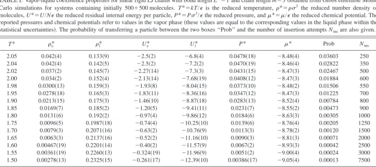
Although it is commonly assumed that molecular flex-ibility has little effect in terms of the fluid phase behavior, recent work has questioned this.1Hence, we start by consid-ering the effect of flexibility on the fluid phase transitions. In Fig. 1共a兲 the T*-* phase diagrams for model systems of chains with three tangent LJ segments are presented. Com-puter simulations of the fully flexible 3CLJ system were car-ried out previously by Blas and Vega;23,53they report a criti-cal point at T*⫽2.06 and*⫽0.088. Here, we have carried out GEMC simulations for the corresponding rigid system 共see the previous section for details of the simulations兲; the critical point in this case is found to be Tc*⫽2.081⫾0.016, Pc*⫽0.060⫾0.017, and c*⫽0.089⫾0.004. A comparison between the two simulation studies suggests a slightly higher critical temperature value for the rigid system, although this is difficult to confirm given the 共relatively兲large error asso-ciated with our estimation of the critical temperature from computer simulations. Away from the critical point, little dif-ference is observed for the coexistence densities of the two models. As we will see later, the effect of flexibility is more noticeable for larger chains. In Fig. 1共a兲the result of a cal-culation with the TPT1 of Wertheim for Lennard-Jones chains22,23is also presented for comparison. The theory gives a very good description of the phase behavior of the system for the entire phase envelope, although larger deviations are seen in the region close to the critical point, as expected from any classical equation of state.
In Fig. 1共b兲the T*-*phase diagram for LJ chain
mol-ecules with m⫽5 tangent segments is presented. We
ob-tained the phase envelope for linear rigid molecules using GEMC simulations 共see the previous section兲, and find the critical conditions at Tc*⫽2.49⫾0.06, Pc*⫽0.034⫾0.012, andc*⫽0.046⫾0.009. Unfortunately, no simulation data are available for the flexible model. As comparison we have in-cluded in the figure the vapor-liquid envelope obtained with
the TPT1 of Wertheim. Blas and Vega53 showed that the
approach provides an excellent description of the phase be-havior of flexible LJ chain molecules. Assuming that the the-oretical calculations represent the phase behavior of the
flex-ible model in the case of m⫽5, we can conclude that a
widening of the T*-* envelope is seen as a result of an
TABLE VI. Zero-pressure densities*of linear rigid LJ chains in the CP1 solid phase as obtained from NPT Monte Carlo simulations for m⫽3 and 5.
m T* *
3 1.05 0.3411
3 1.00 0.3433
3 0.95 0.3452
3 0.90 0.3473
3 0.85 0.3493
3 0.80 0.3512
5 2.05 0.1999
5 2.00 0.2006
5 1.95 0.2017
5 1.90 0.2025
5 1.85 0.2035
5 1.80 0.2044
TABLE VII. Coexistence densities, pressures, and chemical potentials at T*⫽4 used as starting states for the Gibbs–Duhem calculations.
m T* P* l* s* /(kBT)
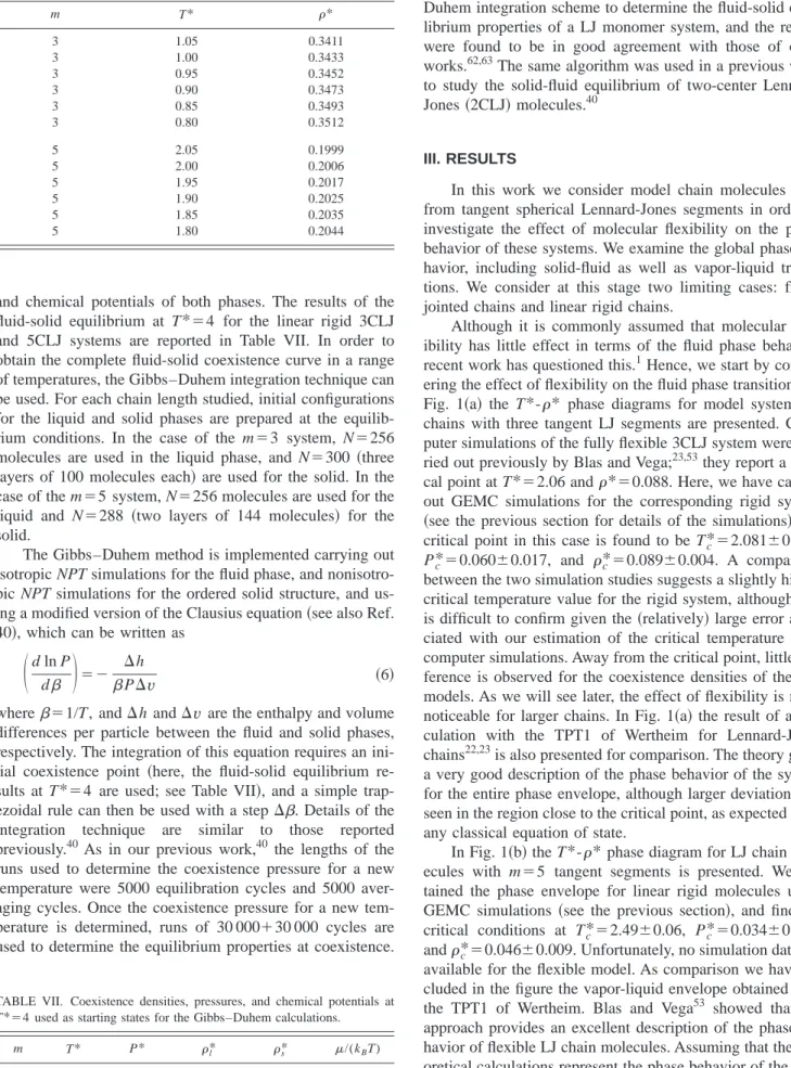
increased stiffness in the chain. The phase diagram in the P*-T* projection is presented in Fig. 2. The vapor pressure curves for the 3CLJ and 5CLJ systems are shown. The simu-lations carried out in this work for the linear rigid models are compared with calculations using the TPT1 approach of Wer-theim, which can be considered as accurately representing a flexible chain model. The flexible and rigid 3CLJ models exhibit vapor pressure curves which are very close, as could be expected given the T*-* diagram of Fig. 1共a兲. In the case of the 5CLJ systems, a slight difference in vapor pres-sure is noted between the flexible and rigid systems. The results presented in Figs. 1 and 2 seem to suggest that, while little difference is observed in the equations of state of flex-ible and rigid chains of tangent hard spherical segments,17,18 a noticeable difference in the vapor-liquid equilibrium is seen when attractive interactions are also involved.
The simulation data for flexible and rigid models for LJ
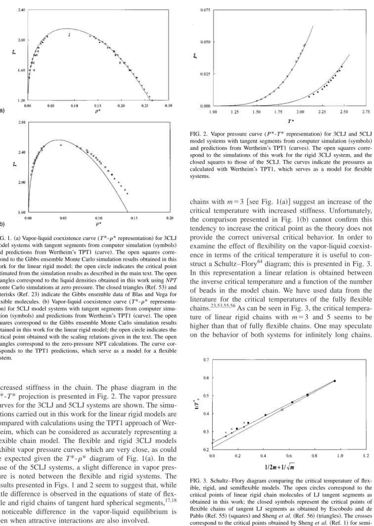
chains with m⫽3 关see Fig. 1共a兲兴 suggest an increase of the critical temperature with increased stiffness. Unfortunately, the comparison presented in Fig. 1共b兲 cannot confirm this tendency to increase the critical point as the theory does not provide the correct universal critical behavior. In order to examine the effect of flexibility on the vapor-liquid coexist-ence in terms of the critical temperature it is useful to con-struct a Schultz–Flory64diagram; this is presented in Fig. 3. In this representation a linear relation is obtained between the inverse critical temperature and a function of the number of beads in the model chain. We have used data from the literature for the critical temperatures of the fully flexible chains.23,53,55,56As can be seen in Fig. 3, the critical
tempera-ture of linear rigid chains with m⫽3 and 5 seems to be
higher than that of fully flexible chains. One may speculate on the behavior of both systems for infinitely long chains.
FIG. 1.共a兲Vapor-liquid coexistence curve (T*-*representation兲for 3CLJ model systems with tangent segments from computer simulation共symbols兲 and predictions from Wertheim’s TPT1 共curve兲. The open squares corre-spond to the Gibbs ensemble Monte Carlo simulation results obtained in this work for the linear rigid model; the open circle indicates the critical point estimated from the simulation results as described in the main text. The open triangles correspond to the liquid densities obtained in this work using NPT Monte Carlo simulations at zero pressure. The closed triangles共Ref. 53兲and asterisks共Ref. 23兲indicate the Gibbs ensemble data of Blas and Vega for flexible molecules.共b兲Vapor-liquid coexistence curve (T*-* representa-tion兲for 5CLJ model systems with tangent segments from computer simu-lation共symbols兲and predictions from Wertheim’s TPT1共curve兲. The open squares correspond to the Gibbs ensemble Monte Carlo simulation results obtained in this work for the linear rigid model; the open circle indicates the critical point obtained with the scaling relations given in the text. The open triangles correspond to the zero-pressure NPT calculations. The curve cor-responds to the TPT1 predictions, which serve as a model for a flexible system.
FIG. 2. Vapor pressure curve ( P*-T*representation兲for 3CLJ and 5CLJ model systems with tangent segments from computer simulation共symbols兲 and predictions from Wertheim’s TPT1 共curves兲. The open squares corre-spond to the simulations of this work for the rigid 3CLJ system, and the closed squares to those of the 5CLJ. The curves indicate the pressures as calculated with Wertheim’s TPT1, which serves as a model for flexible systems.
The critical point of an infinitely fully flexible chain of LJ
tangent segments is found to be T*⫽4.59共as suggested by
Sheng et al.兲. Extrapolating from the GEMC simulations for
linear rigid chains of LJ m⫽3 and m⫽5 tangent segments,
the critical temperature of an infinitely long linear rigid chain is found to be T*⫽5.27; i.e., of the order of 25% higher than that of the flexible model. However, our estimate of the criti-cal temperature of infinitely long linear rigid LJ chains
should be treated with caution since molecules with m⫽3
and 5 are certainly too short to yield linear behavior in a Schultz–Flory plot. Simulation data for longer linear rigid chains are needed to establish definite conclusions in this respect. Our present results seem to suggest that the critical point of infinitely long linear LJ chains may be higher than that of the fully flexible model 共this is certainly the case for
short chains兲, but more work needs to be carried out to
clarify this point completely. It is important to mention also that Sheng et al. examined the critical temperature of semi-flexible model molecules formed by tangent LJ segments. In their model the bond angle was fixed to the tetrahedral value, and a torsional potential was introduced. They showed that such a nonflexible model yields a critical temperature lower than that of the fully flexible case. In this work we have found the opposite共i.e., a higher critical temperature for the linear rigid model兲in comparing to the fully flexible model. This seems to indicate that the way in which chain stiffness is incorporated can affect the critical properties and chemical details of the model共the bond angle in our work is 180° as compared to 109.5° used by Sheng et al.兲. Although, as sug-gested earlier, it may turn out that the linear rigid chains considered here are too short for the Schultz–Flory plot to be valid. For short chains, the critical temperature of linear rigid chains seems to be lower than that of fully flexible chains. For long chains, we have only an indication that the same may be true, and further work is needed in this respect. As a conclusion of this part of the work, it seems clear that
flex-ibility has a non-negligible effect on the vapor-liquid phase behavior of chains with attractive interactions, and that a number of issues are yet to be resolved.
Let us now turn our attention to the solid-fluid equilibria.
In previous work,39 an extension of the TPT1 of Wertheim
was proposed which can be used to model the solid phases of fully flexible chain molecules of LJ tangent segments. The approach provides an excellent description of the global
phase behavior of the 2CLJ system,40 and, although the
phase behavior of longer flexible chains has not yet been compared with computer simulation data, it is useful to re-view here the main findings of the predicted phase behavior of fully flexible LJ chains.39The most striking feature is the existence of an enormous fluid range 共in the limit of infi-nitely long chains the ratio Tt/Tcis 0.14兲. This is due to the fact that the critical temperature of chain molecules increases for increasing chain length, whereas the calculated triple-point temperature remains practically constant; in fact it is seen to decrease slightly for increasing chain length. The stable solid structure for flexible chains of tangent spherical segments is the so-called disordered solid,33,34a solid struc-ture in which the spherical segments are arranged in a close packed fcc lattice with no long-range orientational order be-tween bond vectors. The stable solid structure of a system of rigid chains, however, corresponds to an ordered arrange-ment of layers with the molecular axes of all the molecules in a layer pointing in the same direction 共i.e., the CP1 struc-ture兲. Since the equilibrium solid structure is different for both models, and since the Hamiltonian of both systems is certainly different, one may expect important differences in the fluid-solid equilibrium of both systems.
We have used the Gibbs–Duhem integration technique to obtain the fluid-solid coexistence curve in a range of tem-peratures共Tables VIII and IX兲for linear rigid LJ chain mol-ecules. At low temperatures the solid densities along the sub-limation curve can be estimated from the zero-pressure
TABLE VIII. Fluid-solid coexistence properties obtained using the Gibbs–Duhem integration scheme for linear rigid LJ chain molecules of bond length L*⫽1 and chain length m⫽3. The initial equilibrium point for the Gibbs–Duhem integration was a state at T*⫽4 and P*⫽35.108.*f ands*are the fluid
and solid densities at fluid-solid coexistence, respectively.
T* P* *f s* T* P* f* s*
simulations presented previously 共Table VI兲. The global phase diagrams obtained from simulation are presented in Figs. 4 (T*-* projection兲 and 5 ( P*-T* projection兲. The triple-point temperature can be estimated from the simulation
results by extrapolating the fluid-solid coexistence tempera-tures to zero pressure共i.e., the vapor-liquid-solid triple-point pressure is expected to be very small兲. Conversely, it can also be determined by finding the temperature at which the den-sity of the fluid at zero pressure becomes identical to that of the fluid in the fluid-solid coexistence curve. The triple-point temperatures and densities for the linear rigid 3CLJ system are Tt*⫽1.040, l*⫽0.281, and s*⫽0.342. For the linear rigid 5CLJ system these are Tt*⫽2.050,l*⫽0.122, ands*
⫽0.199. In a previous work the triple point of the 2CLJ
system was found40 to be Tt*⫽0.650, l*⫽0.462, and s* ⫽0.515共note that for the 2CLJ the stable solid structure at the triple point is a disordered one兲. In contrast with the phase behavior of flexible chains, a clear stabilization of the solid phases results from increasing chain lengths in these rigid systems. The triple-point temperature increases dra-matically, faster, in fact, than the increase seen for the critical point. As a result, the region of vapor-liquid coexistence de-creases. The Tt*/Tc* ratio is 0.50 for the chain with three segments, while it is 0.82 for the five-segment chain. By comparison, the fluid range of flexible molecules of similar chain lengths, as predicted by our theoretical approach,39 is of the order of 0.30. Another indication of the stabilization of the solid phases is the shift toward lower densities in the fluid-solid transition 关see especially Fig. 4共b兲兴, and the wid-ening of the density gap. These results are in agreement with
FIG. 4. Global phase diagram in 共a兲 T*-* and 共b兲 T*-s* 共where s*
⫽*m) representations for linear rigid chain molecules of three and five tangent LJ segments as obtained from the simulations of this work. The open symbols correspond to the 3CLJ system and the closed symbols to the 5CLJ system. The squares correspond to the results of GEMC calculations, the triangles to the NPT calculations of the liquid phase at zero pressure, the circles to the solid-fluid coexistence densities obtained with Gibbs–Duhem calculations, and the asterisks and crosses to the solid densities obtained with NPT calculations at zero pressure.
FIG. 5. Global phase diagram in P*-T*representation for linear rigid chain molecules of three and five tangent LJ segments as obtained from the simu-lations of this work. See Fig. 4 for details of the symbols.共b兲shows the P*-T*projection at low pressures共the lines are guides to the eyes兲. TABLE IX. Fluid-solid coexistence properties obtained using the Gibbs–
Duhem integration scheme for linear rigid LJ chain molecules of bond length L*⫽1 and chain length m⫽5. The initial equilibrium point for the Gibbs–Duhem integration was a state at T*⫽4 and P*⫽6.58.*f ands*
are the fluid and solid densities at fluid-solid coexistence, respectively.
T* P* f* s*
4 6.5800 0.1648 0.2001
3.7037 5.4647 0.1638 0.1994
3.4483 4.5300 0.1615 0.1996
3.2258 3.7296 0.1571 0.1979
3.0303 3.0531 0.1564 0.1964
2.8571 2.4625 0.1516 0.1982
2.7027 1.9504 0.1473 0.1954
2.5641 1.5104 0.1475 0.1982
2.4390 1.1156 0.1437 0.1989
2.3256 0.7697 0.1384 0.1987
2.2222 0.4634 0.1333 0.1990
2.1276 0.1976 0.1278 0.1993
the simulations of Polson and Frenkel.36In Fig. 5 the P*-T* projections of the phase diagrams as obtained from simula-tion are shown for the 3CLJ and 5CLJ systems. At a fixed pressure the solid-liquid melting temperature is displaced to higher temperatures for increasing chain length. As before, this corresponds to a stabilization of the solid phase. In Fig. 5共b兲 the shift of the triple-point temperatures can be better observed. A comparison of the phase behavior of linear and flexible chains can be seen in Fig. 6. The phase behavior of the flexible model is obtained with the TPT1 approach pre-sented in earlier work.39It can be clearly seen in Fig. 6 that in the case of the flexible model the predicted triple-point temperature remains practically constant for increasing chain lengths; this leads to the large fluid range seen in the flexible model systems. Using the distance fluctuation criterion for melting and computer simulations, Zhou et al.31,32noted that the results obtained with clusters of square-well segments and isolated square-well homopolymers are very similar, and suggest that chain connectivity does not affect the solid-liquid equilibrium in the case of freely jointed chains; our TPT1 model seems to lead to the same conclusion. In the rigid systems, however, the marked stabilization of the solid phases results in an increase of the triple-point temperatures and the shrinkage of the fluid range.
It is encouraging to see that the trends highlighted here
for the rigid chains confirm the predictions of our theoretical calculations for chains of tangent hard segments interacting via attractive dispersion interactions treated at the mean-field level of van der Waals.48In the former work a simple exten-sion of Wertheim’s theory is coupled with a scaling argument to take into account the fewer degrees of freedom of a rigid
chain 共as compared to a flexible chain兲. As regards the
theory, the stabilization of the solid phase with respect to the fluid is explained in terms of this loss of degrees of freedom. It was also suggested that, as a result of the marked increase in the triple-point temperature, the vapor-liquid envelope would be metastable in systems of long rigid chains with attractive interactions. An extrapolation of the values of the Tt*/Tc*ratio as obtained from simulation in our present work suggests that chains with more than six segments will not exhibit stable vapor-liquid transitions共see Fig. 7兲. In the fig-ure the ratios corresponding to flexible LJ chains as predicted
by the extension of Wertheim’s theory37 are also shown for
comparison. In the flexible systems, the liquid-vapor enve-lope not only does not become metastable for any chain length, but dominates the phase diagram.
A final point should be made before finishing this sec-tion. As discussed in the Introduction, it has been shown3,4 that linear rigid chain molecules of tangent hard segments exhibit liquid crystalline phase behavior for chain lengths equal to or larger than five segments. In particular, Vega et al.4 have studied the phase behavior of the system with five tangent segments using NPT computer simulations. Fol-lowing a compression route, they observed isotropic, nem-atic, smectic A, and solid phases. The hard system is related to the behavior of the LJ system at high temperatures共where the effect of attractions is small兲. Therefore, since linear rigid hard sphere chains form liquid crystals, one may expect that LJ linear rigid chains may also form liquid crystal phases共at least at high temperatures兲. However, in the simulations
per-formed in this work for m⫽5 and T*⫽4 in the fluid phase
no evidence of liquid crystal phase formation was found. It remains to be considered if liquid crystal phases will appear
for this model with m⫽5 at higher temperatures. De Miguel
FIG. 6. Global phase diagram in共a兲T*-*and共b兲P*-T*representations for linear rigid chain molecules of three and five tangent LJ segments as obtained from the simulations of this work and compared with TPT1 calcu-lations共Ref. 39兲. The solid lines correspond to the TPT1 calculations for the flexible chains and the symbols to the simulation points of the rigid systems. See Fig. 4 for details of the symbols.
FIG. 7. Sketch of the Tt/Tcratio for varying chain length in model chains
and Vega29 presented the global phase diagram of a Gay– Berne model system which includes solid, liquid crystalline, and fluid phases. In their chosen system a solid-nematic-fluid triple point is observed at relatively high temperature, and a second solid-liquid-vapor triple point is observed at low tem-peratures. We expect that a similar phase diagram may emerge for the system of linear rigid LJ molecules if high enough temperatures are studied; we will consider this point in future work.
IV. CONCLUSIONS
We have determined the global phase behavior 共
vapor-liquid and fluid-solid equilibria兲 of linear rigid chain mol-ecules of three and five tangent LJ segments using computer simulations. The vapor-liquid equilibria were determined us-ing Gibbs ensemble Monte Carlo simulations and isobaric-isothermal 共NPT兲 calculations at zero pressure. In order to determine the fluid-solid coexistence densities at a given temperature, we obtained the free energies of each phase by thermodynamic integration. For the solid phase, this first re-quired calculating the free energy at a particular共solid兲state point. The Gibbs–Duhem integration technique was then used to obtain the solid-fluid transition at various tempera-tures. Zero-pressure NPT simulations have also been carried out at very low temperature to determine the coexistence solid densities along the sublimation curve. We have studied the effect of flexibility on the phase behavior by comparing the phase diagrams of flexible and rigid LJ chains.
The vapor-liquid critical conditions obtained in this work are found to be Tc*⫽2.081⫾0.016, Pc*⫽0.060⫾0.017, and c*⫽0.089⫾0.004 for the linear rigid 3CLJ system, and Tc* ⫽2.49⫾0.06, Pc*⫽0.034⫾0.012, andc*⫽0.046⫾0.009 for the linear rigid 5CLJ system. In respect to the vapor-liquid coexistence, we find that flexible and rigid chains of LJ seg-ments exhibit noticeable differences. This is a rather unex-pected result, as the equation of state of linear and rigid chains of tangent hard segments are very similar.18The criti-cal temperature of linear rigid LJ chains is found to be higher than that of flexible chains of corresponding chain length. In the limit of chains of infinite length, the difference is of
about 25%共assuming the Schultz–Flory plot can be used for
the short chains considered here兲.
As far as the fluid-solid phase equilibria are concerned, a clear stabilization of the solid phase with respect to the fluid is seen for increasing chain lengths; both the solid and fluid
densities at coexistence 共even when expressed in monomer
units兲 shift toward lower densities for larger molecules. To-gether with this, a marked increase of the triple-point tem-perature is observed: the triple-point temtem-peratures and den-sities for the linear rigid 3CLJ system are Tt*⫽1.040, l* ⫽0.281, ands*⫽0.342, while for the linear rigid 5CLJ sys-tem these are Tt*⫽2.050, l*⫽0.122, and s*⫽0.199. As a result of the stabilization of the solid phase, the fluid range 共given by the ratio Tt/Tc) decreases for increasing chain length, and it is predicted to disappear for chains with more than six tangent LJ segments. This is in marked contrast with the phase behavior predicted for systems of flexible LJ chains of tangent segments.37 In the flexible molecular
sys-tems, the vapor-liquid coexistence was seen to dominate the phase diagram. To explain this one must take into account two factors. First, the equilibrium solid structure of fully flexible and linear rigid chains is completely different. Rigid linear chains freeze into an ordered arrangement of layers with all the molecules in a layer pointing in the same direc-tion, while the stable solid structure of a system of fully flexible chains of tangent spherical segments is one with no long-range orientational order of bonds.
Second, the difference of the Hamiltonian does also af-fect the equation of state in the solid phase. It has been shown previously that even if a CP1 structure is ‘‘imposed’’ on a fully flexible chain in the solid phase, its equation of state differs from that of the rigid linear chain41in the same CP1 solid structure. Therefore the difference of the Hamil-tonian affects the equation of state, even if the same solid structure is considered.
To summarize the content of this paper one may say that linear rigid LJ chains present a shrinkage of the liquid range, and that fully flexible LJ chains present a huge liquid range (Tt/Tc⫽0.14). The behavior of semiflexible molecular
sys-tems 共such as n-alkanes兲 is expected to lie somewhere
be-tween these two extremes. In future work we plan to con-sider longer rigid chains and examine the phase behavior in more detail, analyzing the possibility of liquid crystal forma-tion in these systems.
Note added in proof. Please note there was a misprint in Table I of Ref. 39. ai j for i⫽4, j⫽1 should be 69.214 instead of 68.219 as reported.
ACKNOWLEDGMENTS
Financial support is due to Projects No. BFM-2001-1420-C02-01 and No. BFM-2001-1420-C02-02 of Spanish
DGICYT 共Direccio´n General de Investigacio´n Cientı´fica y
Te´cnica兲. A.G. would also like to thank the Engineering and Physical Sciences Research Council for the award of an Ad-vanced Research Fellowship. E.S acknowledges the award of a FPU grant. L.G.M. acknowledges the award of a Ramon y Cajal grant. E.d.M. and F.J.B. would also like to thank Uni-versidad de Huelva and Junta de Andalucı´a for additional financial support.
1
Y. J. Sheng, A. Z. Panagiotopoulos, and S. K. Kumar, Macromolecules 29, 4444共1996兲.
2P. Paricaud, A. Galindo, and G. Jackson, Mol. Phys. 101, 2575共2003兲. 3D. C. Williamson and G. Jackson, J. Chem. Phys. 108, 10 294共1998兲. 4
C. Vega, C. McBride, and L. G. MacDowell, J. Chem. Phys. 115, 4203
共2001兲.
5R. Dickman and C. K. Hall, J. Chem. Phys. 85, 4108共1986兲. 6D. Frenkel, J. Phys. Chem. 92, 3280共1988兲.
7L. Onsager, Ann. N.Y. Acad. Sci. 51, 627共1949兲. 8
G. J. Vroege and H. N. W. Lekkerkerker, Rep. Prog. Phys. 55, 1241
共1992兲.
9H. Finewever and A. Yethiraj, J. Chem. Phys. 108, 1636共1998兲. 10M. R. Wilson, Mol. Phys. 81, 675共1994兲.
11
M. S. Wertheim, J. Stat. Phys. 35, 19共1984兲.
12
M. S. Wertheim, J. Stat. Phys. 35, 35共1984兲.
13M. S. Wertheim, J. Stat. Phys. 42, 459共1986兲. 14M. S. Wertheim, J. Stat. Phys. 42, 477共1986兲. 15M. S. Wertheim, J. Chem. Phys. 87, 7323共1987兲. 16
W. G. Chapman, G. Jackson, and K. E. Gubbins, Mol. Phys. 65, 1057
共1988兲.
18C. Vega, C. McBride, and L. G. MacDowell, Phys. Chem. Chem. Phys. 4,
853共2002兲.
19P. J. Flory, Proc. R. Soc. London, Ser. A 234, 73共1956兲. 20
W. G. Chapmanf, J. Chem. Phys. 93, 4299共1990兲.
21J. K. Johnson, J. A. Zollweg, and K. E. Gubbins, Mol. Phys. 78, 591
共1993兲.
22J. K. Johnson, E. A. Mu¨ller, and K. E. Gubbins, J. Phys. Chem. 98, 6413
共1994兲.
23
F. J. Blas and L. F. Vega, Mol. Phys. 92, 135共1997兲.
24L. A. Davies, A. Gil-Villegas, and G. Jackson, Int. J. Thermophys. 19, 675
共1998兲.
25A. Gil-Villegas, A. Galindo, P. J. Whitehead, S. J. Mills, G. Jackson, and
A. N. Burgess, J. Chem. Phys. 106, 4168共1997兲.
26
L. A. Davies, A. Gil-Villegas, and G. Jackson, J. Chem. Phys. 111, 8659
共1999兲.
27E. A. Mu¨ller and K. E. Gubbins, Equations of State for Fluids and Fluid Mixtures共Elsevier, Amsterdam, 2000兲.
28
E. A. Mu¨ller and K. E. Gubbins, Ind. Eng. Chem. Res. 40, 2193共2001兲.
29E. de Miguel and C. Vega, J. Chem. Phys. 117, 6313共2002兲.
30I. A. Solov’yov, A. Solov’yov, W. Greiner, A. Koshelev, and A. Shutovich,
Phys. Rev. Lett. 90, 053401共2003兲.
31
Y. Zhou, M. Karplus, J. Wichert, and C. K. Hall, J. Chem. Phys. 107, 10691共1997兲.
32Y. Zhou, M. Karplus, K. D. Ball, and R. S. Berry, J. Chem. Phys. 116,
2323共2002兲.
33K. W. Wojciechowski, D. Frenkel, and A. C. Branka, Phys. Rev. Lett. 66,
3168共1991兲.
34K. W. Wojciechowski, A. C. Branka, and D. Frenkel, Physica A 196, 519
共1993兲.
35C. Vega, E. P. A. Paras, and P. A. Monson, J. Chem. Phys. 96, 9060
共1992兲.
36
J. M. Polson and D. Frenkel, J. Chem. Phys. 109, 318共1998兲.
37C. Vega and L. G. MacDowell, J. Chem. Phys. 114, 10411共2001兲. 38C. McBride and C. Vega, J. Chem. Phys. 116, 1757共2002兲.
39C. Vega, F. J. Blas, and A. Galindo, J. Chem. Phys. 116, 7645共2002兲. 40
C. Vega, C. McBride, E. de Miguel, F. J. Blas, and A. Galindo, J. Chem. Phys. 118, 10696共2003兲.
41E. Sanz, C. McBride, and C. Vega, Mol. Phys. 101, 2241共2003兲. 42
H. C. Longuet-Higgins and B. Widom, Mol. Phys. 8, 549共1964兲.
43E. P. A. Paras, C. Vega, and P. A. Monson, Mol. Phys. 79, 1063共1993兲. 44F. J. Blas, A. Galindo, and C. Vega, Mol. Phys. 101, 449共2003兲. 45
E. D. Nikitin, High Temp. 36, 305共1998兲.
46D. L. Morgan and R. Kobayashi, Fluid Phase Equilib. 63, 317共1991兲. 47C. Vega and C. McBride, Phys. Rev. E 65, 052501共2002兲.
48
F. J. Blas, E. Sanz, C. Vega, and A. Galindo, J. Chem. Phys. 119, 10958
共2003兲.
49V. A. Ivanov, M. R. Stukan, M. Mu¨ller, W. Paul, and K. Binder, J. Chem.
Phys. 118, 10333共2003兲.
50M. P. Allen and D. J. Tildesley, Computer Simulation of Liquids共
Claren-don, Oxford, 1987兲.
51
G. S. Dubey, S. O’Shea, and P. A. Monson, Mol. Phys. 80, 997共1993兲.
52J. Stoll, J. Vrabec, H. Hasse, and J. Fischer, Fluid Phase Equilib. 179, 339
共2001兲.
53
F. J. Blas and L. F. Vega, J. Chem. Phys. 115, 4355共2001兲.
54A. Z. Panagiotopoulos, Mol. Phys. 61, 813共1987兲.
55F. A. Escobedo and J. J. de Pablo, Mol. Phys. 87, 347共1996兲. 56
Y. J. Sheng, A. Z. Panagiotopoulos, S. K. Kumar, and I. Szleifer, Macro-molecules 27, 400共1994兲.
57A. Perera and F. Sokolic, Mol. Phys. 88, 543共1996兲. 58
C. Vega, E. P. A. Paras, and P. A. Monson, J. Chem. Phys. 97, 8543
共1992兲.
59M. Parrinello and A. Rahman, Phys. Rev. Lett. 45, 1196共1980兲. 60
S. Yashonath and C. N. R. Rao, Mol. Phys. 54, 245共1985兲.
61D. Frenkel and A. J. C. Ladd, J. Chem. Phys. 81, 3188共1984兲. 62M. A. van der Hoef, J. Chem. Phys. 113, 8142共2000兲. 63
R. Agrawal and D. A. Kofke, Mol. Phys. 85, 43共1985兲.