Estudio e implementación de un modem digital GFSK aplicado a comunicaciones móviles

Texto completo

(1).,..,,.-. -·.. INSTITUTO TECNOLÓGICO Y DE ESTUDIOS SUPERIORES DE MONTE~Y CAMPUS ESTADO DE MÉXICO 1 ;'{. :. ·. 21 SEF Z?3l.f.o·1. ESTUDIO E IMPLEMENTACIÓN DE UN MODEM DIGITAL GFSK APLICADO A COMUNICACIONES MÓVILES. DIGITAL GFSK MODEM STUDY, DESIGN AND IMPLEMENT ATION APPLIED TO MOBILE COMMUNICATIONS. TESIS QUE PARA OPTAR EL GRADO DE MAESTRO EN CIENCIAS DE LA INGENIERIA PRESENTA. DANIEL SANTANA GOMEZ. Asesor: Comité de tesis:. Jurado:. Dr. JAVIER EDUARDO GONZALEZ VILLARRUEL Dr. LUIS FERNANDO GONZALEZ PEREZ Dr. ANDRES DA VID GARCIA GARCIA Dr. Dr. Dr. Dr.. LUIS FERNANDO GONZALEZ PEREZ, ANDRES DA VID GARCIA GARCIA, JAVIER EDUARDO GONZALEZ VILLARRUEL ALDO GUSTAVO OROZCO LUGO. Atizapán de Zaragoza, Estado de México. Enero de 2005.. Presidente Secretario Vocal Vocal.

(2) 4. RESUMEN. Esta Tesis presenta el estudio, el análisis y la implementación de un Modem GFSK sobre una plataforma DSP (Digital Signal Processor) aplicado a comunicaciones móviles. Este trabajo representa el inicio del análisis e implementación de un demostrador de Software-radio. El proyecto presenta un análisis de las modulaciones digitales más utilizadas en comunicaciones inalámbricas, un análisis detallado de la modulación FSK-GFSK por medio de simulaciones en Matlab y la implementación en el DSP TMS320C5416 de Texas Instruments. En este trabajo de Tesis, se han analizado, simulado e implementado: un modulador FSK de fase continua, filtros pasabajas y gaussiano, un demodulador FSK no-coherente y un algoritmo de decisión de tipo IaD (Integrate and Dump). Finalmente se presenta el análisis de la implementación a más altas velocidades con ADC-DAC disponibles en el Mercado y se presenta la comparación entre el sistema simulado y el sistema implementado.. ABSTRACT. This Thesis presents a GFSK Modem implementation on a DSP (Digital Signal Processor) platform applied to mobile communications. It is the beginning of a future implementation of a complete Software-radio setup. The project presents an analysis of the most used digital modulations in wireless communications, a detailed analysis of GFSK modulation based on Matlab simulations and the implementation in a TMS320C5416 Texas Instruments DSP. Within this Thesis, it is analyzed, simulated and implemented: a FSK continuous phase modulator, low pass and Gaussian filters, a non-coherent FSK demodulator and an IaD (Integrate and Dump) decision algorithm. Finally the analysis of the implementation at high rates with available ADCDAC is presented together with the comparison between the simulated system and the implemented system..

(3) 5. CONTENTS. ACKNOWLEGMENTS. 3. RESUMEN. 4. ABSTRACT. 4. CONTENTS. 5. LIST OF FIGURES. 9. LIST OF TABLES. 11. l. INTRODUCTION. 12. 1.1 MOTIVA TION. 12. 1.2 OBJECTIVES. 13. 1.3 STATE OF THE ART. 13. 1.4 ORGANIZATION OF THE THESIS. 13. 1.5 BIBLIOGRAPHY. 14. 2. DIGITAL MODULATIONS SCHEMES APPLIED TO WIRELESS SYSTEMS. 15. 2.1 WIRELESS COMMUNICATION SYSTEM. 15. 2.2 LINEAR AND NON LINEAR MODULATION TECHNIQUES. 16. 2.3 LINEAR MODULATIONS. PUASE SHIFT KEYING (PSK). 17. 2.3.1 QPSK (QUADRA TURE PSK) 2.3.2 n/4-DQPSK (DIFFERENTIAL QUADRA TURE PHASE SHIFT KEYING). 17 18.

(4) 6 2.4 LINEAR MODULATIONS. QUADRA TURE AMPLITUD E MODULATION (QAM). 20. 2.5 NON LINEAR MODULATIONS. FREQUENCY SHIFT KEYING (FSK) 2.5. l GAUSSIAN FREQUENCY SHIFT KEYING (GFSK). 20 21. 2.6 NON LINEAR MODULATIONS. MINIMUM SHIFT KEYING (MSK) 2.6. l GAUSSIAN MINIMUM SHIFT KEYING (GMSK). 21 22. 2.7 BANDWIDTH AND POWER EFFICIENCY ANALYSIS. 22. 2.8 APPLICATIONS OF MODULA TION SCHEMES. 24. 2.9 CONCLUSIONS. 25. 2.10 BIBLIOGRAPHY. 25. 3. DIGITAL SIGNAL PROCESSORS. 26. 3.1 PROGRAMMABLE PLATFORM COMPARAISON AND SELECTION. 26. 3.2 TEXAS INSTRUMENT TMS320CX DIGITAL SIGNAL PROCESSORS FAMILY. 28. 3.3 TMS320C5416 SPECTRUM DIGITAL DSP STARTER KIT (DSK). 30. 3.4 PCM3002 CODEC. 31. 3.5 DSP SOFTWARE TOOLS. CODE COMPOSER STUDIO. 32. 3.6 CONCLUSIONS. 33. 3.7 BIBLIOGRAPHY. 33. 4. GFSK MODEM ANALYSIS. 34. 4.1 GFSK MODULATOR 4.1.l SINE TABLE GENERATION 4.l.2 CONTINUOUS PHASE FSK 4.l.3 GAUSSIAN FILTER. 34 36 37 38. 4.2 DEMODULATOR 4.2.1 NON-COHERENT DEMODULATION LIMITATIONS 4.2.2 DECISION ALGORITHM. 39 43 45. 4.3 CONCLUSIONS. 46. 4.4 BIBLIOGRAPHY. 46. 5. SIMULATION. 47. 5.1 MATLAB SIMULATION OF A GFSK MODEM AT 9.6 KHZ 5.1.l GFSK MODULA TION 5.l.2 POWER SPECTRUM DENSITY (PSD) 5.1.3 DEMODULA TION 5.1.4 TRANSMISSION THROUGH AN ADDITIVE WHITE GAUSSIAN NOISE (AWGN). ERROR PERFORMANCE (BER). 47 49 50 52. 54.

(5) 7 5.2 MATLAB SIMULA TION OF A GSFK MODEM AT 2 MHZ (ONE BLUETOOTH CHANNEL) 5.2.1 MODULA TION 5.2.2 MODULATION POWER SPECTRUM DENSITY (PSD) 5.2.3 DEMODULA TION 5.2.4 TRANSMISSION THROUGH AN ADDITIVE WHITE GAUSSIAN NOISE (A WGN). ERROR PERFORMANCE (BER). SS 57 58 59. 5.3 CONCLUSIONS. 61. 5.4 BIBLIOGRAPHY. 61. 6. DSP IMPLEMENTATION. 62. 6.1 IMPLEMENTATION DETAILS. 63. 6.2 MODULA TOR. 63. 6.3 DEMODULATOR. 67. 6.4 CONCLUSIONS. 69. 6.5 BIBLIOGRAPHY. 70. 7. CONCLUSIONS ANO RESULTS. 71. 7.1 MATLAB SIMULATION VERSUS DSP IMPLEMENTATION. 71. 7.2 DSP TIMING ANALYSIS. 73. 7.3 HIGH SPEED IMPLEMENTATION ANALYSIS. 74. 7.4 THESIS IMPACT AT ITESM. 75. 7.5 IMPLEMENTATION CONCLUSIONS. 75. 7.6 FUTURE WORK. 75. 7.7 BIBLIOGRAPHY. 75. APPENDIX A. 77. l. SINE TABLE. 77. II. MATLAB MODULATOR FUNCTION. 80. III. GAUSSIAN FILTER MAGNITUD E AND PUASE RESPONSE. 82. IV. MATLAB DEMODULATOR FUNCTION. 83. APPENDIX B. 86. I. MODEM MAIN FUNCTION. 86. 11. MODULATOR (MOD_DATA). 92. 59.

(6) ~I. 8 111. DEMODULATOR (DELAY_INPUT). 93. IV. INCLUDED FILES A. SINE TABLE B. GAUSSIAN FILTER COEFFICIENTS (MODULA TOR) C. LOW PASS FILTER COEFFICIENTS (DEMODULA TOR). 94 94 96 96. V. GAUSSIAN FILTER AMPLITUD E AND PHASE RESPONSE. CODE COMPOSER PLOTS.. 98. VI. LPF FILTER AMPLITUDE AND PHASE RESPONSE. CODE COMPOSER PLOTS.. 99.

(7) 9. LIST OF FIGURES. Figure2.1 General wireless communication system Figure2.2 General Modulator Figure2.3 BPSK signals Figure2.4 QPSK constellation diagram Figure2.5 n:/4-QPSK Constellation diagram Figure2.6 16QAM constellation diagram Figure2. 7 FSK signals Figure2.8 MSK signals Figure2.9 Power Spectral Densities ofFSK, 16QAM, BPSK and MSK (a) linear (b) logarithmic. Figure2.1 OBandwidth and power efficiency plot Figure3.1 Programmability and specialization comparison of programmable devices Figure3.2 DSPs vendors Figure3.3 TMS320Cx Family ofDSP's Figure3.4 C5000 DSP Platform Roadmap [1] Figure3.5 TMS320C5416 DSK Architecture Figure3.6 PCM3002 architecture Figure3.7 Code Composer Studio devefopment environment [4] Figure4.1 GFSK Modulator Figure4.2 Coherent and Non coherent FSK Figure 4.3 FSK frequencies distribution. Figure4.4 Sine signals for different k, a) k=l, f=l, b) k=5, f=500 Hz, c) k=21, f=2 KHz Figure4.5 FSK continuous phase modulation Figure4.6 Gaussian Filter impulse response Figure4. 7 FSK Demodulator Figure4.8 Non-coherent FSK demodulator Figure4.9 Demodulator signals: a) Binary input, b) R(n), c) Rd(n), d) Rt(n) Figure4.1 Oa Demodulator performance with a n:/2 delay Figure4.1 Ob Demodulator performance without a n:/2 delay Figure4.11 Bit rate (fh) versus sample frequency (fs) Figure4.12 fb and fs behavior Figure 5.1.Frequency frequencies for integer k.. 15 16 17 18 19 20 21 22 23 24 26 28 29 29 30 31 32 35 35 36 37 38 39 40 40 41 42 43 44 44 48.

(8) 10 Figure5.2 Modulation Flow Chart 49 Figure5.3 FSK and GFSK output 50 Figure5.4 FSK and GFSK PSD 51 Figure5.5 FSK and GFSK PSD with higher fs 51 Figure5.6 Demodulator flow chart 52 Figures. 7 a) GFSK demodulated signal and data input, b) GFSK demodulated signal after the 53 comparator, e) GFSK demodulated signal after IaD Figure5.8 GFSK signals with noise. a) GFSK demodulated signal and data input, b) GFSK 54 demodulated signal after the comparator, e) GFSK demodulated signa) after IaD Figure5.9 GFSK with IaD Probability of error compared with FSK non-coherent demodulation and with FSK coherent demodulation. 55 Figure5.10 Bluetooth GFSK modulation 57 Figure5.11 a) FSK signals b) GFSK signals 58 Figure5.12 GFSK after decision algorithm 59 Figure5.13 BER versus SNR in GFSK modulation 60 Figure6.1 DSP modulator flow chart 64 Figure6.2 GFSK modulation 65 Figure6.3 FSK spectrum 65 Figure6.4 Mirror effect in GFSK modulation 66 Figure6.5 FSK and GFSK spectrum 66 Figure6.6 DSP demodulator Flow chart 67 Figure6. 7 Modem GFSK setup 68 Figure6.8 GFSK Demodulator output 68 Figure6.9 GFSK demodulator with IaD 69 Figure 7.1 GFSK modulation PSD a) DSP, b) Matlab 72 Figure7.2 GFSK demodulator signals. a) DSP, b) Matlab 72 FigureAl. Gaussian Filter response at 9600bps Modem 82 FigureA2. Gaussian Filter response in lMbps (Bluetooth) Modem 82 FigureA3. Low Pass Filter responses in 9600 bps Modem 85 FigureA4. Low Pass Filter responses in 1Mbps Modem (Bluetooth) 85 FigureB 1. Gaussian Filter magnitude response in time domain 98 FigureB2. Gaussian Filter amplitude and phase response in frequency domain 98.

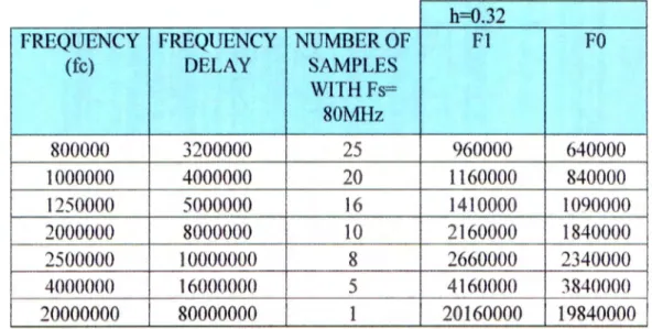
(9) 11. LIST OF TABLES. Table2.1 n:/4-DQPSK Phase-change correspondence bits ........................................................... 19 Table2.2 Modulation Applications ............................................................................................. 24 Table3.1 Performance, cost, power, flexibility and design complexity comparison of programmable devices ....................................................................................................... 27 Table5.1. GFSK parameters with h=0.4375 ................................................................................ 48 Table5.2 GFSK parameters with h=0.32 .................................................................................... 56 Table6.1 DSP implementation parameters .................................................................................. 62 Table7.1. Implementation function profile ................................................................................. 73 Table7.2 Maximum bit rate ofimplemented modem .................................................................. 74 Table7.3 High-speed codec's, application and maximum bit rate ............................................... 74.

(10) 12. l. INTRODUCTION. This Thesis is part of the research work developed for the Mobile Communications Chair of the Electric Department at the ITESM campus Estado de México. The Research work of the Chair concems the development of 4th Generation Mobile Communications WLAN (Wireless Local Area Network) Systems and Architectures development. The Chair aims to generate specialized human resources in the coding, modulation, radio frequency and integrated circuits related to Mobile Communications. In this Thesis we have focused in the analysis and development of modulation techniques. Modulation techniques as OFDM, QPSK, QAM, GMSK and GFSK among others are used in specific areas of mobile communications as IMT-2000, GSM, GPRS, WCDMA, IEE802.l l and Bluetooth [l]. These modulations combined with multiple access techniques allow having more users and faster systems. In other hand, Software Defined Radios (SOR) perform signal-processing task by running software algorithms on multi-purpose Digital Signal Processors (DSPs). Flexibility offered by DSPs facilitates efficient integration of multiple standards, such as Bluetooth and WLAN, on a single radio system [2]. Then the main goal in this Thesis is the implementation of a wireless Digital Modem under the Bluetooth Standards applied to WPANs over dedicated platforms (Digital Signal Processors platform based).. 1.1 MOTIVA TION The number of different standards for mobile communication is increasing and thus a need for a universal and flexible transceiver becomes more apparent. Then the need for a programmable transceiver for multiple standards requirements is fundamental and transcendental research. The improvements in digital signal processor (DSP) technology and ADC/DAC technology are undergoing rapid advances [3]. More advantages using software rather than implementing in hardware are the ability to easily upgrade and reuse. A software-defined radio is a radio where the ADC and DAC are performed as close as possible to the antenna. This implies that the demodulation/modulation and signal processing are to be performed by software in the digital domain. This project presents a software radio implementation; it considers the modulation and demodulation stages. The familiarization with the DSP tools, performance and optimization is an important fact in this work thinking in future projects..

(11) 13. 1.2 OBJECTIVES. The objective of this Thesis is to implementa modem in a DSP platform. Gaussian Frequency Shift Keying (GFSK) modulation scheme is the one to be implemented. This modulation is the modulation used in the Bluetooth standard and can be the used to generate other WPANs and WLANs modulation schemes like Gaussian Minimum Shift Keying (GMSK), Phase Shift Keying (PSK) and Quadrature Amplitude Modulation (QAM) [8].. 1.3 STATE OF THE ART. Demand of future wireless communication services will require an always-on connection according to the Quality of Service QoS and provider service. This QoS involve multiple wireless standards that require intelligent and dynamic portable device. Wireless modems are key part of mobile devices in adequate transmissions according to QoS. In order to adapt different wireless standard, future radios will need to be implemented on software format. Thanks to DSP and wireless technologies, today software modem radios for 2 and 2.5 Generations have already been implemented [3,4]. In other hand, the DSPs implementations have been growing as improves the performance of these. These improvements combined with the development of faster ADC-DAC circuits allow more applications to be implemented. The modulation scheme to be studied, simulated and implemented in this thesis is the Gaussian FSK modulation, used in Bluetooth technology. It is a low-cost, low-power, short-range radio that communicates data and voice in point-to-multipoint networks from 0-10 meters up to 1 Mbps by WPANs [5]. As adoption rates of Bluetooth functionality continues to rise in mobile phones and other devices, it will be essential part in communications of 4G as a devices communications utility. The most significant improve to Bluetooth in this times is the inclusion of Medium Data Rate (MOR) in an updated standard. At present Bluetooth connections run ata relatively modest 720Kb/s, 12 times faster than a modem but over 100 times slower than a LAN connection [6]. The idea is that Bluetooth's data speed increases two or three orders of magnitude. It will allow most devices connected like notebook PC, personal digital assistant (PDA), cell phone even cars and refrigerator, in a short range.. 1.4 ORGANIZATION OF THE THESIS The outline of this Thesis is as follows. After this introduction Chapter 2 present an introduction of a Digital Modulations Schemes used in wireless systems. The chapter presents an overview of the schemes and a bandwidth and power analysis. Chapter 3 describes the main features of the Digital Signal Processors focused in the TMS320C5000 family of Texas Instruments. Chapter 4 presents a theoretical analysis of the GFSK modem. In Chapter 5 a simulation in Matlab is presented based on the theory in Chapter 4. A 9600 bps GFSK modem has been simulated and then a modification for 1Mbps Bluetooth channel. Chapter 6 presents the DSP implementation details of the 9600 bps GFSK modem and finally in Chapter 7 conclusions and results are.

(12) 14 presented. Appendix A and B present the programs, filters response and sine table of simulation and implementation respectively.. 1.5 BIBLIOGRAPHY. [1] T. S. Rappaport; "Wire/ess Communications:Princip/es and Practices"; Second Edition, Prentice Hall, 2002. [2] Jeffrey H. Reed, "Software Radio. A modern approach to radio engineering", Prentice Hall, USA, 2002. [3] Roel Schiphorst, Fokke Hoeksema, and Kees Slump, "Channel Se/ection Requirements for Bluetooth Receivers using a Simple Demodulation Algorithm ", PRORISC workshop, 29-30 November 2001, Veldhoven, Netherlands, November 2001. [4] Charles Tibenderana, Stephan Weiss, "A Low-Complexity High-Performance Bluetooth Receiver", in Proceedings of IEE Colloquium on DSP enabled Radio, pages pp. 426-435, Livingston, Scotland, Department of Electronics and Computer Science, University of Southampton, UK, 2003. [5] Kristina Bengtsson, "A DSP based Bluetooth solution, Department of Te/ecommunications and Signa/ Processing", Master Thesis, Blekinge Institute of Technology. [6] Bluetooth Special Interest Group, "Specification of the Bluetooth System ", February 2002, Core. [7] Keith E. Nolan, Linda Doyle, "Modulation Scheme Classification for 4G Software Radio Wireless Networks", in Proceedings of the !ASTED Intemational Conference on Signal Processing, Pattem Recognition, and Applications (SPPRA 2002), June 25-28, 2002, Crete, Greece, pp25-31 [8] Daniel Santana, Javier Gonzalez, "Digital Modulation DSP analysis and implementation based on integer k-sampling", in ICED 2004, Internacional Conference on Electronic Design, Veracrúz, Veracrúz, Nov. 21 -22..

(13) 15. 2. DIGITAL MODULATIONS SCHEMES APPLIED TO WIRELESS SYSTEMS. Digital modulation compared to analog modulation is more robust to noise and interference impairments inherent in wireless channels, more power and spectral efficient modulations, however may be more complex and expensive implementations [1]. This chapter presents a brief review of linear and non-linear digital modulations applied to wireless communications systems, in the first part we study the principal linear and non-linear digital modulations, then in the second part the power and spectral efficiencies are study, and finally in the last part the principal wireless communications systems and modulations are presented. The conclusion at the end of the chapter allows us to present the digital modulation best suited for our application.. 2.1 WIRELESS COMMUNICATION SYSTEM. A fundamental wireless communication system involves the information transmission using a wireless channel [2]. Figure 2.1 shows a general wireless communication system.. ~~. Source. L~_Jl:r--_encoder. Channel. encoder. Modulator. Channel. Analog. output. Source decoder. Channel. decoder. Demodulator. Figure2.1 General wireless communication system.

(14) 16 Due to inherent hostile channel characteristics, a wireless system requires multiple signal processing stages as source coding, channel coding, interleaving, band pass modulation and in a spectral limited digital system burst processing. For most of the advanced wireless systems, the air interface and band pass modulation are the more critical and complex stages to implement in the case of software radios, due to spectral efficiency, interferences between wireless systems, etc. For this reason, this work address band pass modulation. Band pass modulation is a process that allows to impresses a digital symbol onto a signal suitable for transmission in a wireless channel. In the case of wireless communication, digital modulation is more suitable that analog modulation due to its noise performance and improved processing techniques. This chapter will allow us to study the digital modulations techniques in order to define best suited for our work. Digital modulation can be regrouped as nonlinear and linear where the first are non-constant envelope in contrast with the last where a constant envelope can be obtained.. 2.2 LINEAR AND NON LINEAR MODULATION TECHNIQUES A general modulator is shown in Figure 2.2. The linearity and non-linearity is depending on the relation between the input and the output of the system [3].. Input (modulating signal) m(t}. MODULATOR. Output (modulated signal) ____ ... S{t). --. a. Sinusoidal Carrier c(t) Figure2.2 General Modulator Linear Modulation: • The input-output relation of modulator satisfies the "Principie of Superposition" (2.2.1 ). It is that the output (S) produced by a number of inputs (in) applied simultaneously is equal to the sum of the output that result when the inputs are applied one at a time. If the input is scale by a certain factor, the output of the modulator is scaled by exactly the same factor [4]. (2.2.1).

(15) 17 No Linear Modulation: •. Input-Output relation of modulator does not (partially or fully) satisfies the principie of superposition. In other terms, a linear modulation is the one where bits encoded in amplitude (P AM), phase (PSK) or both (MQAM) with no constant envelope. In Nonlinear Modulations, the bits are encoded in frequency (FSK) with constant envelope so they are less susceptible to amplitude and phase nonlinearities introduced by the channel and/or hardware [4]. This chapter shows the Linearity and nonlinearity importance in theoretical and practica! aspects. Firstly linear modulations are described, then nonlinear and finally a spectrum analysis of them is shown.. 2.3 LINEAR MODULATIONS. PHASE SHIFT KEYING (PSK) The basic kind of Phase Shift Keying (PSK) is the Binary PSK (BPSK) in where binary data are represented by two signals with different phases. Typically these phases are Oand n:, the signals are represented by: So(t) = Acos2111/J. Os t s T. for I (2.3.1). s1(t) = -Acos2m/J. Os t s T. forO. The waveform has a constant envelop and its frequency is constant too. In Figure 2.3 is shown that a "1" causes a phase transition, and a "O" does not produce a transition.. BINARYDATA. o. o. o. BPSK MODULATED SIGNAL. So. So. S1. S1. So. Figure2.3 BPSK signals. 2.3.1 QPSK (QUADRATURE PSK). To increase the bandwidth efficiency of PSK, the MPSK scheme was delivered. In BPSK, a data.

(16) 18 bit is represented by a symbol, in MPSK, n=log2M data bits are represented, thus the bandwidth efficiency. ji_= log 2 M. w. [ bits Is I Hz] increases n times.. Quadrature PSK (QPSK) is the most often used MPSK (M=4) scheme because it doesn't suffer from BER degradation while the bandwidth efficiency is increased. So, if we define four signals, each with a phase shift differing by 90° then we have a quadrature phase shift. The signals are defined by:. s;(t) = Acos(2TifJ + 0¡),. OstsT. i = 1,2,3,4 (2.3.2). where (J. = -'-( 2_i----'1)_Jr 1. 4. A constellation diagram that is an X-Y display, which shows the data states of phase, or phaseamplitude encoded data of modulation. Figure 2.2 shows the constellation diagram of a QPSK modulation. There can be noted that the position is at 45° it means that Q gains and J are ±1/v'2, so the magnitude of the carrier will never exceeds 1.. Figure2.4 QPSK constellation diagram. 2.3.2 ,w:/4-DQPSK (DIFFERENTIAL QUADRA TURE PHASE SHIFT KEYING) QPSK modulation presents sorne problems as zero crossings and wide spectrum, rr/4-QPSK reduces sorne of these problems by limiting the phase changes and spectrum utilization. Differential means that the information is not carried by the absolute state; it is carried by the transition between states. Then, in rr/4-DQPSK the carrier trajectory does not go through the.

(17) 19 origin and there can be transition from any symbol position to any other symbol position. The transmitted signal in rc/4-DQPSK has the form:. x(t) = cos(wJ+ cp(t)). (2.3.3). Where <j>(t) is the phase term that carries the information and it is constant overa symbol period, therefore:. for kT s t s (k + l)T. x(t) = cos(wJ + </Jk). (2.3.4). The rc/4-DQPSK modulation carries two bits of information per symbol. The data-phase-change correspondence for the two bits of information is shown in Table 2.1.. Symbol. o 1. 2 3. Table2.1 rc/4-DQPSK Phase-change correspondence bits GrayCode Sign bitof Sign bitof A+k si.DA+ cosA+k rc/4 00 o o 01 3rc/4 o 1 11 -3rc/4 1 1 -rc/4 10 1 o. The constellation diagram of a rc/4-DQPSK modulation is shown in Figure 2.5.. o. ,. . ,. Figure2.5 rc/4-QPSK Constellation diagram.

(18) 20. QUADRATURE. 2.4 LINEAR MODULATIONS. MODULATION (QAM). AMPLITUD E. It is simply a combination of amplitude modulation and phase shift keying. It can be expressed. like: s¡(t). = Acos(2J'ifJ + 0¡). i = l,2,3 ... M. (2.5.1). Where A¡ is the amplitude and 8¡ is the phase ofthe ith signal in the M-ary signal set. For example if M= 6 (16QAM), there are four /values and four Q values. Then, its and results in a total of 16 possible states for the signal and the symbol rate is one fourth of the bit rate. It means that four bits per symbol can be sent. 16QAM constellation diagram is shown in Figure 2.6. In QAM a transition from any state to any other state at every symbol time can be done. So this modulation format produces a more spectrally efficient transmission[5]. 0010. 0011. 0001 0000. • • • • 1010 1011 1001 1000 • • • •. • 1101 • 1100 • • 1111 • • • • 0110 0111 0101 0100 1110. Figure2.6 16QAM constellation diagram. The current practica} limits are approximately 256QAM, though work is underway to extend the limits to 512 or 1024 QAM.. 2.5 NON LINEAR MODULATIONS. FREQUENCY SHIFT KEYING (FSK) Binary FSK is the simplest FSK scheme, it use two signals with different frequencies to represent binary symbol "O" and "1 ". No information exists in the amplitude; the information is contained in the frequency. In general form it is represented by: s¡(t). = Acos(2¡ifit + </>). kT s t s (k + l)T, for 1. (2.5.1) kT s t s (k + l)T, for O.

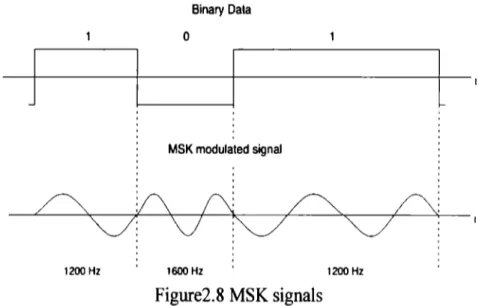
(19) 21 Where cp could be the same for both signals, it is called continuous phase or coherent modulation. If it is different is called non-coherent modulation. The signals of a FSK modulation are shown in Figure 2.7. BINARYDATA. _j. o. o. FSK MODULATED SIGNAL. WVV\Jv lo. 11. lo. 11. lo. Figure2. 7 FSK signals. 2.5.1 GAUSSIAN FREQUENCY SHIFT KEYING (GFSK) Normal continuous phase Binary FSK transmits a "O" as frequency fo and a "1" as frequency f1. This, however, results in an inefficient use of bandwidth dueto the rectangular input data causing sudden frequency transitions in the modulated signal. GFSK deals against this effect by premodulating the input data signal with a Gaussian filter. The Gaussian filter minimizes the instantaneous frequency variations over time.. 2.6 NON LINEAR MODULATIONS. MINIMUM SHIFT KEYING (MSK) MSK is a continuous phase modulation scheme where the modulated carrier contains no phase information and frequency changes occurs at the carrier zero crossings. The difference between the frequency of a "O" and a "l" is equal to half the data rate. lt is the minimum spacing that allows FSK signals to be coherently orthogonal (no interference during process of detection). In other words, MSK is a FSK modulation with a modulation index of 0.5 [6]. Modulation index is defined as: m=At·T. Where:. Ar= Íi - fo and T- V' - / Bitrate. (2.6.1).

(20) 22 Figure 2.8 shows the MSK signals. The peak-to-peak frequency shift of an MSK signal is equal to one-half of the bit rate. FSK and MSK produce constant envelope carrier signals, which have no amplitude variations. This is a desirable characteristic for improving the power efficiency of transmitters. Amplitude variations can exercise nonlinearities in an amplifier' s amplitude-transfer function, generating spectral re-growth, a component of adjacent channel power. Therefore, more efficient amplifiers (which tend to be less linear) can be used with constant-envelope signals, reducing power consumption.. Binary Dala. o. j. t MSK modulated signal. vv~ '. '\J: '. ''. ''. 1200 Hz. 1600 Hz. ' '. 1200 Hz. ' '. Figure2.8 MSK signals. 2.6.1 GAUSSIAN MINIMUM SHIFT KEYING (GMSK) GMSK is derived of MSK where the bandwidth required is further reduced by passing the modulating waveform through a Gaussian filter. The Gaussian filter minimizes the instantaneous frequency variations over time. GMSK is a spectrally efficient modulation scheme and is particularly useful in mobile radio systems. lt has a constant envelope, spectral efficiency a good BER performance and is self-synchronizing.. 2.7 BANDWIDTH AND POWER EFFICIENCY ANALYSIS There is no single class of modulation technique that is suitable for all applications, since communications channels and performance requirements vary widely. The conventional classification of various modulation schemes is based on their power and bandwidth utilization efficiencies. The power spectral density (attenuation of the power spectrum at a specified separation from the center frequency) is then so important in the selection of a modulation technique [4]. Figure 2.9 shows the Power Spectral Density of the modulations techniques that we are considering. In blue is the FSK PSD with h=l.4, in magenta the BPSK PSD, in green the MSK PSD with h=0.5 and in red the QAM-MPSK PSD..

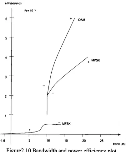
(21) 23. 1". 0.8. E:0.6. ..,. \. \. [l_. \. 0.4. 0.2. o o. 0.2. 0.4. 0.6. 1.2. 0.8. 1.4. 1.6. f. a) o. 0.5. 1.5 f. 2. 2.5. (b) Figure2.9 Power Spectral Densities of FSK, 16QAM, BPSK and MSK (a) linear (b) logarithmic.. We can see that the FSK modulation is the most bandwidth inefficient but the simplest to detect. MSK is a FSK variation with h=0.5 and it is more bandwidth efficient than BPSK but no than QAM. The second plot shows the nodules of the modulated signal. Because 16QAM uses more symbols it the one with the shortest nodules. With these plots is difficult to see the power efficiency then Figure 2.1 O presents an analysis based on the bandwidth and the power efficiency..

(22) 24 Pe= 10 -~. 6. 5. 4. + MPSK. 3. 2. , - - - - - MFSK + -1.6. 5. 10. 15. 20. 25 El)INo(aB). Figure2.1 O Bandwidth and power efficiency plot When M increases MFSK is power efficient, but not bandwidth efficient. In the other hand MPSK and QAM are bandwidth efficient but not power efficient. With the newest Gaussian techniques like GMSK and GFSK, the bandwidth inefficiency of the frequency modulation is being reduced. So, these modulations are still power efficient but now the bandwidth inefficiency is reduced. Then, because of the low-complexity implementation they have been used for a several wireless applications, the most representative GSM in the case of GMSK and Bluetooth in the GFSK case.. 2.8 APPLICATIONS OF MODULATION SCHEMES Table 2.2 shows the main applications of each modulation scheme. Tabl e2.2 Mod ulaf10n A.pp li cat1ons. MODULATION SCHEME MSK, GMSK BPSK QPSK, :rt/4 DQPSK, FSK, GFSK 16QAM 256QAM. APPLICATION GSM,CDPD Deep space telemetry, Cable modems Satellite, CDMA, TETRA, Cable modems Paging, AMPS, land mobile, Bluetooth Microwave digital radio, modems Modems, DVB-C (Europe ), Digital Video (US). So, we can see that there are applications for each modulations scheme, and there is no one that has all the benefits for all the applications [8]. Depending on the application is the modulation.

(23) 25 scheme that is selected, in the terms of the bandwidth and power limitations, and complexity of implementation (that is reflected in cost). That's why the PSK and QAM modulations are used mainly in the bandwidth-limited systems, the FSK in the power limited systems.. 2.9 CONCLUSIONS Because the power efficiency and the low-complexity demodulation implementation, FSK modulation was selected to the first implementation. Having a FSK implementation is easily the transition to a MSK and a binary PSK. In other hand, a Gaussian Filter implementation is considered too. Having it, GFSK and GMSK could be generated. It could guide us throw the future implementation of a multiple standards Software Radio. In this work we will be focused in a GFSK modulator and demodulator implementation based on the Bluetooth norm that is being developing for a short-range wireless communications. Bluetooth uses Gaussian frequency shift keying (GFSK) with a modulation index between 0.28 and 0.35. In the next chapters the simulation and implementation will be shown.. 2.10 BIBLIOGRAPHY [l] Fuqin Xiong, "Digital Modulation Techniques ", Artech House, USA, 2000. [2] T. S. Rappaport; "Wireless Communications"; Prentice Hall, 2002. [3] Ambreen Ali, Felicia Berlanga "Linear vs Constant Envelope Modulation Schemes in Wireless Communication Systems", Report, University ofTexas in Dallas. [4] Dr. Mike Fitton, "Telecommunications Research Lab ", Report, Toshiba Research Europe Limited. [5] Leon W. Couch 11, "Modern Communication Systems. Principies and Applications ", Prentice Hall, 1995. [6] HP application note 1298, "Digital Modulation in Communications Systems- An lntroduction ", USA, 1997. [7] Kevin C. Yu, Andrea J. Goldsmith, "Linear Models and Capacity Bounds for Continuous Phase Modulation ", in IEEE Intemational Conference on Communications, pp. 722-726, April 2002. [8] Geoff Smithson, "Jntroduction to Digital Modulation Schemes ", IEE Colloquium on The Design of Digital Cellular Handsets, London, UK, page(s): 2.1-2.9, 4 Mar 1998..

(24) 26. 3. DIGITAL SIGNAL PROCESSORS. In this chapter a brief introduction to digital signal processors DSP is provided. DSPs are digital programmable device well suited for communication applications. As DSPs, ASICs and FPGAs are also programmable devices that can be used to implement digital functions. After this introduction, a brief comparison between these devices is provided, then a description of different DSP and components, the tools to program the DSP and finally the description of the DSP used in this project.. 3.1 PROGRAMMABLE PLATFORM COMPARAISON AND SELECTION With the technology progress various programmable platforms are available for digital functions implementations. In our case, we are interested in mobile communications applications where real time complex functions at low power consumption are required. Various programmable devices as ASICs, FPGAs and DSPs can be used to implement these specific functions. Figure 3.1 shows a comparison of the programmability and specialization between the main programmable devices for Digital Signal Processing applications.. Programmabllity. 1 Specialization. Figure3.1 Programmability and specialization comparison of programmable devices.

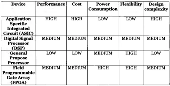
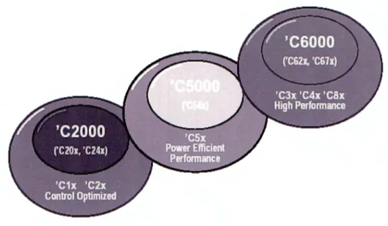
(25) 27 Other comparison based on the cost, flexibility, performance, power consumption and complexity of design is shown in Table 3.1.. Table 3.1 Performance, cost, power, flexibility and design complexity comparison of prograrnmable devices Device. Performance. Cost. Power Flexibility Design Consumption complexity. Application Specific Integrated Circuit (ASIC) Digital Signal Processor (DSP) General Propose Processor Field Programmable GateArray (FPGA). HIGH. HIGH. LOW. LOW. HIGH. MEDIUM. MEDIUM. MEDIUM. MEDIUM. MEDIUM. LOW. LOW. MEDIUM. HIGH. LOW. MEDIUM. MEDIUM. HIGH. HIGH. MEDIUM. As can be noted in table 3.1, DSPs are the most suitable device for our case, since their capability to implement more complex design at lower power consumption. ASICs and FPGAs are normally used for specific applications that require in addition a superior operation and a good tradeoff in terms of performance and power. In contrast the DSP platform looks more flexible and has less restrictions in terms of power or performance limitations. Also, DSPs are more flexible to re-prograrnmable. There are severa} companies that produce DSP like Texas Instruments, Motorola, Hitachi and Toshiba. Figure 3.2 shows the top 10 vendors of Embedded Prograrnmable Processors Product Mix in 2000. Texas Instruments have the largest share of market in DSP devices, followed by Lucent and Motorola. Texas Instruments DSPs are produced for any market and have the widest range of applications. Lucent and Motorola are working together and have many potential costumers. For this work, we have selected a Texas Instrument DSP of the family TMS320C5000. This platform is user friendly for communication applications and has been optimized in digital processing and low power consumption. In order to understand more about Texas Instruments DSPs this chapter shows a general description of the Texas Instrument TMS320 families and a particular description of the C5000 family..

(26) 28 Mllllona ol U.8. Dollars. 5.000---------------------------... 4.000. D. DSP. 3.000. 0. '1CU. •. E t>e<loed MiérOprOC9SSOr. Figure3.2 DSPs vendors. 3.2 TEXAS INSTRUMENT TMS320CX DIGITAL SIGNAL PROCESSORS FAMILY. Each generation of TMS320Cx devices uses a core central processing unit (CPU) that is combined with a variety of on-chip memory and peripheral configurations. These various configurations satisfy a wide range of needs in the worldwide electronics market. When memory and peripherals are integrated with a CPU into one chip, the overall system cost is greatly reduced, and circuit board space is reduced. Texas lnstruments have been developing three important families of Digital Signal Processors: The TMS320C2x family oriented to control applications, the TMS320C5000 family oriented to power efficient performance and the TMS320C6000 oriented to a high performance. Figure 3.3 shows the progression of the TMS320Cx devices. With power consumption as low as 0.45 mA/MHz and performance up to 600 MIPS, the C5000 DSP platform is optimized for portable media and communication products like digital music players, GPS receivers, portable medical equipment, feature phones, modems, 3G cell phones, and portable imaging..

(27) 29. Figure3.3 TMS320Cx Family of DSP's [1]. The platform highlights are: • • • • •. Performance up to 900 MIPS Ultra-low-power down to 0.33mA/MHz - enabling incredible new potential for power-sensitive portable systems A wide-range of devices with a rich array of peripherals allows designers to accurately target system needs Complete code-compatibility across all devices, allows reuse of existing code to greatly reduce development burden Reduced time-to-market with a complete development environment and support from Third-Party Network. Figure 3.4 shows the C5000 roadmap where the different applications depending on the devices are showed.. Figure3.4 C5000 DSP Platform Roadmap [1].

(28) 30. 3.3 TMS320C5416 SPECTRUM DIGITAL DSP STARTER KIT (DSK) The TI TMS320C54x DSP is a low power line of DSPs introduced by TI in June 1998. These chips use 16 bit fixed point words, and can run atas low as .45 mW, or at 120 mW at 200 MIPS. The TMS320VC54 l 6 DSP Starter Kit is a stand-alone development and evaluation module. The module is an excellent platform to develop and run software for the TMS320VC5416 family of processors. Figure 3.5 shows the DSK architecture. With 64K words of on board RAM memory, 256K words of on board Flash ROM, anda Burr Brown PCM 3002 stereo codee, the board can sol ve a variety of problems as shipped. Three expansion connectors are provided for interfacing to evaluation circuitry [2]. The hardware features of the DSK are: • Operating at 16-160 MHz • Embedded USB JT AG controller • PCM3002 stereo codee • 64K words of on board RAM • 256K words of on board Flash ROM • 3 Expansion connectors (Memory Interface, Peripheral Interface, and Host Port Interface) • On board IEEE 1149.1 JTAG connection for optional emulator debug • 4 user definable LEDs • 4 position dip switch, user definable • +5 Volt operation only, power supply included • Size: 8.25" x 4.5" (210 x 115) mm), 0.062" thick, 6 layers. Emlle<lded USB JTAG Controller. • D. D A E. s s. 1 D. •T • 1. e o N. JTAG DATA SRAM 64K X 16 ADDRESS. T A. o. TMS320VC5416. L. DECODE. E X. p. FPGA. •. CONTROL. N. s 1. o N. McBSP. Flash ROM 256K X 16. McBSP McBSP. HPl-IO. User. SWitell. User LEOS. DATA. Figure3.5 TMS320C5416 DSK Architecture.

(29) 31. 3.4 PCM3002 CODEC PCM3002 codee is fabricated on a highly advanced CMOS process. lt is a low cost single chip stereo audio CODEC (analog-to-digital and digital-to-analog converters) with single-ended analog voltage input and output. The ADC and DAC employ delta-sigma modulation with 64X over sampling. The ADC includes a digital decimation filter, and the DAC include an 8X over sampling digital interpolation filter. The DAC also include digital attenuation, de-emphasis, infinite zero detection and soft mute to forma complete subsystem. PCM3002 provides a powerdown mode that operates on the ADC and DAC independently. PCM3002's programmable functions are controlled by software [3]. Figure 3.6 shows the architecture of PCM3002 Codee.. Lcllln Analog Front-End Rcllln. Lcll OUt Rcll OUt. Low Pass Filter and output Buffer. Dena-Sigrna Modulator. Mulli-Level Delta-Sigma Modulator. Digital Decirnalion Filler. Digital lnterpolalion Filler. Digital OUI. Figure3.6 PCM3002 architecture. The main features ofthe CODEC are: • • •. •. • •. 16-bit input/output data Software control Stereo ADC: o Single-Ended Voltage Input o 64X Oversampling o High Performance o SNR: 90dB o Dynamic Range: 90dB Stereo DAC: o Single-Ended Voltage Output o Analog Low Pass Filter o 64X Oversampling o High Performance o SNR: 94dB o Dynamic Range: 94dB Sampling Rate: Up To 48khz Single +3V Power supply. Digital In. Serial Interface ano Mode COntrol. -. serial Mooe Control. -. systern Clock.

(30) 32. 3.5 DSP SOFTWARE TOOLS. CODE COMPOSER STUDIO DSP can be programmed either in C code or assembly code. Writing programs in C require less effort but it has minor efficiency that writing programs in assembly. Taking as efficiency, the use of less instruction as possible in a code. In practice, one starts with C coding to analyze the behavior and functionality of an algorithm. Depending of the results, the parts of the code that are making abad function are detected and changed to assembly. If it doesn't take a considerable effect, then all the code has to be changed to assembly code [5]. After that a code is written, software is used to make an executable file. DSPs of TI use software called Code Composer Studio (CCS) that provides a integrated development environment (IDE) to perform the process of assembling, linking, compiling, and debugging steps. The C compiler compiles a source code (.c) to produce an assembly source file (.asm). The assembler is used to make an object file. Then a linker combines the object file as instructed by the command file to create the output file, which will be run in the DSP [6]. The Code Composer Studio (CCS) has graphical capabilities and supports real-time debugging. A number of debugging features are available; including setting breakpoints and watching variables, viewing memory, registers and mixed C and assembly code, graphing results, and monitoring execution time. Real-time analysis can be performed using realtime data exchange (RTDX) associated with DSP/810S. RTDX allows for data exchange between the host, the target and analysis in real time without stopping the target. JT AG emulation interface to control and monitor program execution is available too [4].. Asn~7. Compiler. Edit. Asm -. standard Rtlltime Libraries. l. DSK. Link. r. 1. Config Tool. DSP/BIOS Libraries. DSP/BIOS. SIM. EVM. XDS DSP. Board Figure3.7 Code Composer Studio development environment [4].

(31) 33 DSP/BIOS, is a configuration tool used in Code Composer to generate code to configure pheriphericals, memory, interrupst, timers and almost all the DSK features. It is an alternative form to program the DSK features but in a more effortless way.. 3.6 CONCLUSIONS In this chapter we have presented a brief description of DSP, then a comparison with other programmable platforms as ASIC and FPGA in arder to evaluate the suitability of DSP for our applications. Once the DSP platform has been selected, the characteristics of the implementations tools for the specific platform have been presented. The TMS320C5000 family was selected for our implementation, then the TMS320C5416 DSK has been used as a stand-alone development and evaluation module. Based in this DSK, we have developed a series of programs for the TMS320C5416 family, these programs can be simulated as hardware and software using the Code Composer Studio and the PCM 3002 CODEC.. 3. 7 BIBLIOGRAPHY [1] Texas Instrurnents, "TMS320C5000 Technical Brief ", Technical Reference, ID# SPRU197D, 1999. [2] "TMS320VC5416 DSK", Spectrurn Digital Technical Reference, 2002. [3] Texas Instrurnents, "16-/20-Bit Single-Ended Analog Input/Output SoundPlus™Stereo Audio CODECs", Technical Documents, 2000. [4] Texas Instruments, "Code Composer Studio User's guide", Technical Documents ID#spru328B, 2000. [5] Nasser Kehtarnavaz, Mansour Keramat, "DSP System Design: Using the TMS3320C6000", Prentice Hall, New Jersey, 2001. [6] Rulph Chassaing, "DSP Applications Using C and TMS320C6x DSK", John Wiley and Sons, USA, 2002..

(32) 34. 4. GFSK MODEM ANALYSIS. In this chapter a Gaussian Frequency Shift Key Modem DSP implemented is presented. As was presented in previous chapters, a GFSK modulation has been selected due to its power-efficient modulation, simplicity to be implement on digital programmable platforms, robustness to wireless channels impairments, low power consumption implementation and ability to be translated to other modulation schemes. GFSK modulation is used in Bluetooth standard for short-distance digital radio connections. Bluetooth standard has been designed to implement robust and low complex wireless communication networks. Low power and low cost are also two major key points for Bluetooth. The Bluetooth standard operates in the ISM (Industrial Scientific and Medical) band, at 2.4 GHz [l]. This is one of free license frequency band available worldwide. The frequency bands may be different from country to country, regarding location and width. In most of Europe and the USA the frequency band lies between 2400 and 2483.5 MHz. The modulation format in the Bluetooth standard is Gaussian-shaped binary frequency shift keying, GFSK, with a BT (Bandwidth, Symbol period) product equal to 0.5 [2]. The data symbol rate is 1 MSymbol/s. The purpose of a binary modulation scheme is to achieve a robust format. This also makes the transceiver less complex and thereby the cost is reduced. The demodulation can simply be done using a non-coherent frequency demodulation. Phase and amplitude are not of importance. After this introduction and once the modulation and DSP platform have been chosen, the theoretical analysis of the GFSK modulation and demodulation will be presented in this chapter. In first place the modulator analysis is presented then the demodulator analysis.. 4.1 GFSK MODULATOR In a wireless GFSK Modulator, the binary data are converted to a non-retum to zero (NRZ) format where a 1 represents a binary "1" and a binary "O" is represented by a -1. Then the data are modulated by a FSK modulator and filtered by a Gaussian Filter. Finally, in wireless applications, the modulated signal enters to the RF section to be transmitted through the air. Figure 4.1 shows a block diagram of GFSK modulator..

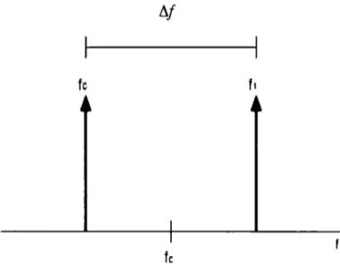
(33) 35. FSK. Gaussian Filter. Modulator. RF. 1------+----I. Modulated. Signa! BASEBAND. Figure4. l GFSK Modulator. The FSK Modulator is the first component of the GFSK modulator, the FSK modulator is a continuous phase or coherent modulator, that means the modulator conserves the phase whatever transition is from the input data [3]. The FSK modulated signal is represented by:. kT s t s (k + l)T, for 1 (4.1.1). kT s t s (k + l)T, for O. Where cp is the same for both signals. Figure 4.2 shows coherent and non-coherent FSK signals.. BINAAYDATA. o. o. COHERENT FSK MODULATION. NON COHERENT FSK MODULATION. :~ ¡. A. r. A 0. A 0. / \ \ 1\ / 1' 1\. 1¡ \: ¡ \ / 1 \ /. 1 ¡. 1. •V V V V. lo. íl. 1. ',. '· 1. ~. /. v. \. /. \/. \. 0. 1 /'\.)\ 1. ~. /. \. 1 / /. V. r, Figure4.2 Coherent and Non coherent FSK 11. lo. And the modulation index of a FSK signal is expressed by:. \ 1: \ '/. 'e. ro.

(34) 36 (4.1.2). Where 1:if is the frequency separation between fo and f1. distribution along the frequency plane [4].. Figure 4.3 shows the frequencies. 1:if. f1. fe. fe. Figure 4.3 FSK frequencies distribution.. Then, fo and f1, can be defined in function of 1:if and fe as follows:. Ío,fi =fe+. ¼. 11. (4.1.3). Coherent FSK signal improves the bandwidth efficiency and generates a constant envelope. Next section shows a DSP implementation to implementa continuous phase FSK modulator.. 4.1.1 SINE TABLE GENERATION As already mentioned for FSK signals, the frequency is the modulation parameter to be mapped by the data; in our case we have also considered a coherent modulation (continuous phase). Continuous phase FSK modulation can be generated from a table for n sinusoid values; different frequencies are generated based on the table steps [5]. The sine table values are calculated with the following expressions:. . (2nn) N. X=Sin--. n = {l,2,3 ...}. (4.1.4).

(35) 37 Where N is the length of the table, and n is the digital variable. To find the length N an interval fs/N needs to be selected, where fs is the sampling rate of the codee. For the DSP (DSK5416), the codee sampling rate is fs=48kHz, then intervals offs/N=lOOHz can been selected as N=480. If we take values from the table with a step k = 1, it corresponds to the values of a 1OOHz signal. In other hand, if we take values of the table in steps different to k = 1, the signal frequency will be varying. To find the k that corresponds to a desired frequency we can apply the following expression where f corresponds to the desired frequency:. (4.1.5). Next figure shows the various signals for different k' s.. l b-r- - - - - - - - - - - - - - - - - - - ,. -100 Hz, k=l -. 500 Hz, k=S. 2 kHz, k=21. Figure4.4 Sine signals for different k, a) k=l, f=l, b) k=5, f=500 Hz, e) k=21, f=2 KHz. 4.1.2 CONTINUOUS PHASE FSK. Based on the sinusoidal table its possible to generate frequencies on intervals of fs/N. For a FSK signal with two levels two frequencies f1, and fo are required, then f1 and fo need to be multiples of 1OOHz. Steps for each frequency from the table, are calculated as follows:. k =fo,,• N 0,1. /J. (4.1.6).

(36) 38 To generate a FSK continuous phase signa} the step in the table needs to be selected depending on the input signal. If the input signa} is a "O", the step in the table will be ko, if it is a "l" the step will be k 1 and it will start where the kO step finished [6]. This process will continue for all the input data. Next figure shows the FSK signa} for f 1 = 400 and fo = 2000.. INPUT DATA. 0.5. o -0.5 -1. o. 10. 20. 30. 40. so. 60. 70. 80. 90. 100. 60. 70. 80. 90. 100. FSK DATA. SO t. Figure4.5 FSK continuous phase modulation. 4.1.3 GAUSSIAN FILTER Next block in a GFSK modulator is a Gaussian filter. The Gaussian Filter reduces the adjacent lo bes of modulated signal. This reduces the bandwidth ofthe output signa} and therefore GFSK is more spectrurn efficient compared to nonnal FSK. The Gaussian Filter, however, removes higher frequencies of the modulating signa} and bit energy; this can have a negative effect on the Bit Error Rate (BER). The lowpass Gaussian Filter transfer function can be expressed as follows:. 1ª2 l. -J; n2 2 hc(n) = -ex --n a. (4.1.7). where:. ,Fn(2) a=. --J2B. B = -3db Bandwidth = BTproductxBitrate. The number of taps depends on the length of the variable "n", the length is a tradeoff between time implementation and filter response..

(37) 39 Figure 4.6 shows the transfer function for different values of BT product (bandwidth-time product) [7]. In Bluetooth, the BT product is fixed to 0.5.. Ker=infinity Ke,= O.S Ker= 0.3 Ker= 0.2. ., 1;I. .2. C. E. 0.5. ,et. /. / /. / /. '. / /. '. /. o. 3. 2. 4. '. ' 5. nme (bit periods). Figure4.6 Gaussian Filter impulse response. In order to transfonn the low pass filter to a bandpass filter we need to multiply by the cosine impulse response.. (4.1.8). Then in frequency we have:. (4.1.9). 4.2 DEMODULATOR In the demodulator section, the modulated signal is received by the antenna and transferred toan IF section or baseband by the transceiver. Then the signal is passed though a FSK demodulator and finally throughout a decision algorithm that improves the demodulator perfonnance. Figure 4.7 shows the block diagram ofthe general Demodulator..

(38) 40. -. RF Modulated Signal. --. FSK Demodulator. --. _n______n__f"L. Decision algorithm. --. BASEBAND Figure4. 7 FSK Demodulator. The demodulator use a non-coherent demodulation, it detects the frequency changes and simplify the DSP implementation. Amplitude and phase are irrelevant in this case. lt also reduces complexity and the processing time. The decision algorithm improves the demodulator performance. Next section presents the blocks analysis.. 4.2.1 Non-coherent demodulation GFSK demodulator has been implemented using non-coherent Quadrature Detector or FM discriminator showed in Figure 4.8. The goal of this method is to translate a frequency shift into an amplitude change [8]. This is possible by delaying the input signa] and multiplying it with the original (not time-delayed).. R(t). ~1. --. -- ~. Rt(t}. LPF. .. a. --. Delay. Figure4.8 Non-coherent FSK demodulator. Mathematically the received signal can be represented as follows: R(t) = Acos[(wc ± bw)* t+ q¡]. Where: wc=central frequency, '6w = 11f/2,. (4.2.1).

(39) 41. A simple way to demodulate a FSK signa} is using a delay time demodulator. FSK needs to be delayed and multiplied by the original one. FSK signa} after multiplication by a k-delay version can be written as follows:. Rd( t) = Acos[( we ± ów) * t + <p] * Acos[(we ± ów) * (t - k) + <p]. (4.2.2). = A2 cos[2( we ± ów) * t - ( we ± ów) * k + 2 *<p] + cos[(we ± Dw) * k] Low pass filtering this signal, high frequency terms will be removed and the resulted signa} will be:. Rd( t) = cos( we * k ± Dw * k). (4.2.3). Defining Wc *k equal to rc/2 we have: Rt(t) = cos(n/2 ± ów * k) = sin(Sw * k). (4.2.4). Where a positive or negative constant will result depending on Wc + f)w or Wc - f)w signa} transmitted. Wc + f)w or Wc - f)w correspond to f1 and fo signals from de continuous phase FSK modulator. Figure 4.9 shows all the demodulator signals.. Data Input. Jli[lill :OlJVJ: ílJill O. ~. ~. 00. ~. :~ O. 100. 1~. 1~. 100. R(n). _'. _ O. 00. ~. ~. 00. 00. 100. 1~. 1~. 100. ~. 00. 00. 100. 1~. 1~. 100. Rt(n). n. Figure4.9 Demodulator signals: a) Binary input, b) R(n), e) Rd(n), d) Rt(n).

(40) 42. Delay selection depends of various factors as sarnpling time, bite rate and orthogonally between signals. A trade off is required while less delay time is desirable. A rrJ2 delay defined in (4.2.4) provides the best orthogonally between the frequencies, this produces the following condition:. Wc*k=o/z then,. (4.2.5) 1. k=-4* fe. As mentioned before, k corresponds to sarnpling times and ideally a lower value is desirable. Finally after the demodulation process the original levels need to be recovered; this can be done using a comparator. As can be observed in Figure x c) if the demodulated signal is greater than the threshold a "1" is assigned, else "O" is assigned. Figure 4.10a shows the demodulator output versus the input data with a rr,/2 delay and Figure 4.1 Ob shows the sarne input but without a rc/2 delay. As can be see, the second plot have a lot of errors because the threshold is not centered in zero. In other hand, the first plot has the sarne behavior than the input data.. Data Input vs Demodulated signal ( FSK). 0 .5. o -0.5 -1. o. 20. 40. 60. 80. 100. 120. 140. 160. 180. 160. 180. 200. Demodulated Signa! after the comparator. 0 .8 0 .6 0 .4 0.2. oo. 1. 1. 20. 40. 60. 80. - 100. -. ~. 120. 140. 200. Figure4.1 Oa Demodulator performance with a rc/2 delay.

(41) 43. Data Input vs Demodulated signal (FSK). 0.5. -0 .S. O. 20. 40. 60. 80. 100. 120. 140. 160. 180. 200. Demodoo.ted Signal afler the comparator ~. ~. ~. ~. ~. 0.8. 0.6 0.4 0.2. o O. ~. '. 20. '. 40. ~. '. 60. ~. 1. 80. -. 1. 1. 100. 120. 1. 140. ' 160. - 180. 200. Figure4. l Ob Demodulator performance without a rr,/2 delay. 4.2.1 NON-COHERENT DEMODULATION LIMITATIONS In binary FSK signals demodulation the main limitation is that the bitrate must be at least a half of period of the low frequency. lt is expressed as follows:. jb fo=2. (4.2.6). Then, the bit rate in a channel cannot be more than:. (4.2.7). Another limitation is the sample frequency. Lets make the analysis. In the previous section, we found that several delays k can fit the 1r/2 delay [9]. Figure 4.11, shows a single bit of an input data at certain bit rate (fb),.

(42) 44 to. l l l l l l l l l l 1<::ts,'lb. Figure4.11 Bit rate (fh) versus sample frequency (fs). The number of samples (k) per bit depends on the sample frequency (f5). The last sample of the bit is given by:. (4.2.8). There are two principal parameters to consider, fs and fb: • •. If fb increases, the number of samples k to delay the signal decreases, If fs increases, the number of samples k to delay the signal increases.. These statements are shown in Figure 4.12. to. fo>>. l l l l l k= 1. 1<=2. 1<=3. 1<::ts11b. to. fs>>. llllllll !<=11<=21,;=3. 1<::ts11b. Figure4.12 fb and fs behavior.

(43) 45. As given in this chapter, the non-coherent demodulator needs an integer k delay to have a n/2 delay [10]. With these conditions, the central frequencies available for the integers k's in a system are:. J, = /, e. 4 • kinl. (4.2.9). Where k={l,2,3 ... fs/fb}. This relation fulfills the equation (4.2.5) gave for an integer delay k=l. The limitations here are the ones presented in equation (4.1.2) and in (4.2. 7). Then, solving the 2 equations system:. (4.2.1 O). The central frequency for integers k-delay to have a n/2 delay is:. fs 4•k. fc=-. (4.2.11). Replacing (15) in (14) a general formula is found:. (4.2.12). Therefore, there are three parameters to consider in the reach of a bit rate in this system: • • •. Sample frequency (fs), Modulation index (h) and Sample delay (k).. 4.2.2 DECISION ALGORITHM. To improve the demodulator performance different algorithms can be used. Decision algorithms may take a variety of forms but the simplest type is known as Integrate-and-dump (IaD). This algorithm sums all samples during one demodulated bit period and decides on the output of the sum whether the incoming bit is an 'O' o '1 '. lf the sum is positive a positive level is assigned to the entire bit. If the sum is negative, a 'O' level is assigned to the entire bit. The effects of the IaD will be presented in the following chapter..

(44) 46. 4.3 CONCLUSIONS In this chapter we have presented the GFSK modem theory. Analysis, implementation and simulation have also been presented. Limit and trade offs were also presented. One of the major implementation limitations is the sampling frequency (f5). For the modulator, the main limitation is the length of the sine table related to fs, which limits the generated signals precision. In the demodulator side, the fs is related to the fb. When the fs is increased there will be more samples k available to delay the signal and vice versa. Founding these limitations, the parameters of the modem need to be analyzed and designed. With the parameters, a fully simulation of the modem can be done. This is the object of the following chapter.. 4.4 BIBLIOGRAPHY [1] Bluetooth Special Interest Group, "Specification of the Bluetooth System ", Febraury 2002, Core. [2] Kristina Bengtsson, "A DSP based Bluetooth solution, Department of Telecommunications and Signa/ Processing ", Master Thesis, Blekinge Institute of Technology. [3] Fuqin Xiong, "Digital Modulation Techniques ", Artech House, USA, 2000. [4] Leon W. Couch 11, "Modern Communication Systems. Principies and Applications", Prentice Hall, 1995. [5] Phil Evans, Al Lovrich, "Implementation of a FSK modem using the TMS3 20C17 ", Texas Instrument, Application Report spra080. [6] G. Baudin, F. Virolleau, O. Venard, P. Jardin, "Teaching DSP through the Practica/ Case Study of an FSK Modem ", Texas Instrument Application Report, spra347, ESIEE Paris 1996. [7] T. S. Rappaport; "Wireless Communications: Principies and Practice "; Prentice Hall, 2002.. [8] Roel Schiphorst, Fokke Hoeksema and Kees Slump, "Bluetooth demodulation algorithms and their performance", 2nd Karlsruhe Workshop on Software Radios, pages 99-106, March 2002 University ofTwente, Netherlands, 2002. [9] Charles Tibenderana and Stephan Weiss, "A Low-Complexity High-Performance Bluetooth Receiver", in Proceedings of IEE Colloquium on DSP enabled Radio, pages pp. 426-435, Livingston, Scotland, Department of Electronics and Computer Science, University of Southampton, UK, 2003. [10] Daniel Santana, Javier Gonzalez, "Digital Modulation DSP analysis and implementation based on integer k-sampling", in ICED 2004, Internacional Conference on Electronic Design, Veracrúz, Veracrúz, Nov. 21 - 22 ...

(45) 47. 5. SIMULATION. In this chapter two digital modem simulations are presented. First, a GFSK modem working at 9.6K.Hz is presented. This simulation has been implemented in the DSP. Second, a Bluetooth modem simulation is presented. The Bluetooth case has not been implemented due to DSK limitations, however if the DSK codee sample frequency is increased the implementation for the Bluetooth is realizable. This codee is called "daughter card" and is connected to the DSK through a special connectors. Ali the simulations were performed on Matlab and then translated to DSP code. In another hand, once the module or stages is prograrnmed in language C, the code can easily be translated to the DSP programming language. Sorne specific functions required by the modem, like fft, ber, filler, and psd were developed. After this introduction, the simulations details are presented, then the results after simulation and implementation. All programs used in this chapter are totally presented in Appendix A.. 5.1 MATLAB SIMULATION OF A GFSK MODEM AT 9.6 KHZ. In this section, the 9.6KHz GFSK Modem simulation on Matlab is presented. The first module to be considered is the FSK modulator; in this case an index modulation needs to be selected. The index h=0.4375 has been considered dueto have the next parameters:. ti/= 4200Hz fb =9600Hz.

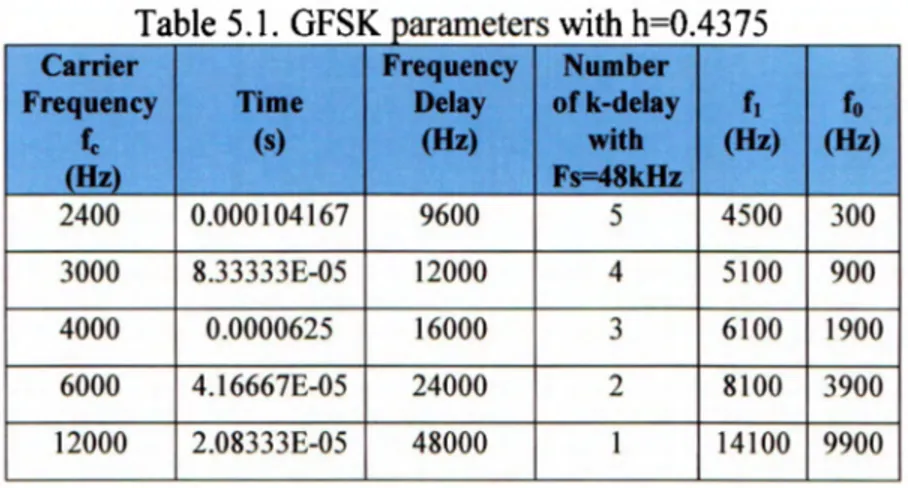
(46) 48 With the DSK sample frequency as 48kHz frequencies fo and f1 can be calculated taking into account the carrier frequency and the integer k delays. Table 5.1 shows the results for different carrier frequencies and rnaxirnum bit rate that could be dernodulated with those frequencies. Tabl e 5.. 1 GFSK parameters w1'th h=O4375. 2400. Frequency Number Delay ofk-delay (s) (Hz) witb Fs=48kHz 0.000104167 9600 5. 3000. 8.33333E-05. 12000. 4. 5100. 900. 4000. 0.0000625. 16000. 3. 6100. 1900. 6000. 4.l6667E-05. 24000. 2. 8100. 3900. 12000. 2.08333E-05. 48000. 1. 14100 9900. Carrier Frequency. fe (Hz). Time. f1. fo. (Hz). (Hz). 4500. 300. Ifthe bit rate is fb=9600 bps. Then the number of samples per bit will be:. -F\ = 48000 = 5 samp les per b'1t. fh 9600. Then, only 5 pair of frequencies with an integer k-delay could be generated in the bandwidth lirnited by the sampling frequency. Those channels are showed in Figure 5.1,. k=5 0.8. k=4 0.6. )(=3 0.4. k=: 0.2. 1r= J. 500). 1(XDJ. 1500J. f. Figure 5.1.Frequency frequencies for integer k.. In our case, we have selected the rninirnum k-delay=l where the rnax bit rate could be reached for a simple channel transmission and where the performance will be improved. A table length of.

(47) 49 N 480 \\as sdecteJ for the nwJulator in orJer to ha,e freyuenc 1 steps of 100 llL 1The \\hole table is pre~enteJ in AppenJi:\ A¡ [ l ]. The rnnstanls for ead1 freyue11e 1 are as foliLms:. 1; • ,\1 9900 • 480 k 1 =-·- = - - - - = 9 9. r. -isooo. I • x 1-i1 oo • -ixo. kll= ~ - - - - - - -=141. F,. 48()()0. 5.1.1 GFSK MODULATION The rvloJulator füm d1an is sho\\n in Figure 5.2. The complete GFSK moJulator has been progranuneJ in i'vlatlab anJ is JetaileJ in AppenJi:\ A.. Stan. Reaó Input NFIZlonnat. 518p = kO. S18p = k1. ... AeaCI step vaJue lrOm. table (Moelutatecl Slgnal). Lengtn table cnack. FIRrou11ne. GauSSlan COIITIICl8n!!. r;;;:;-J. L...:::::..J. Figun:5.2 Modulation Flo,\ Chart.

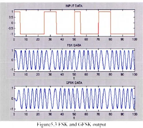
(48) 5U The firsl muJule is the reaJing uf the binar) Jata input. sernnJ muJule rnmpares the input \\ ith a tlueshulJ cenlereJ in Leru anJ assigns the rnrrespunJing slep. founh muJule reaJs the sin table. ne:..! muJule d1ed.s the table length anJ finall) the lasl muJule filters the signa!. The Matlab pwgram \Wrb as fofül\\s, fost a pseuJu ranJum NRZ ::,ey_uence i::, generateJ. then the muJulatur cumpare::, the input NRZ Jata. if the Jata is superiur tu Lew a k.1 ::,lep i::, reaJ fwm the table. iC nul a k.0 is reaJ fwm the table. Then the table length i::, d1eck.eJ tu luup it if the next step is uut uC it. finall) the \alues Crom the table are filtereJ using a Gaussian filler. Gaussian filler I3T parameter has been lixeJ tl> 0.5. I la\ ing this. the fSK l>Utpul is liltered. figure 4.3 sho\b a rnmparisun bemeen the FSK anJ the GFSK forms \er::,us the input Jala.. 1. 0.5. INPUT DATA. -. -. ·-. ;...._. -. o -0.5 -1. o. 10. 20. '. 60. 70. 60. 90. '. 100. 60. 70. 80. 90. 100. 60. 70. 80. 90. 100. 1. 40. 50. FSK DATA. _: o. 10. 40. 20. 50. t GFSK O,,_TA. _: o. 10. 20. 30. 40. 50. t. Figurc5.3 FSK and ( iFSK output. The dTect uf the Gaussian filler can be ::,een in the amplilude uf the FSK ::,igual that i::, reduced in sl>me poinl or the GfSK signa! [2]. GfSK l>Ulpul has a dela) produceJ b) the fIR filler. It is importan! lo Lake illlo acrnulll this Jehi) in the Jeml>dulator I3it Error Anal) sis. As can be ubseneJ un the plul is nut eas) tu ub::,ene the real effect::, (band\\iJthl uf the Gau::,::,ian Filler in time JomaitL therel'on: a Po\\er Spectrum Anal)sÍs must be dl>ne. This is the objecl or the next secliun. The cueHi.cíerns cakulaliun anJ the FIR implemenlatiun are preserned in AppenJix A.. 5.1.2 PO\VER SPECTRU1\I DENSITY (PSD). Figure. ...¡._...¡.. ::,hu\\S the GFSK muJulaliun PSD \er::,u::, the FSK mudulatiun cernereJ al. 1: 12000IIL. As can be obser\eJ from the pll>ls. the Gaussian filler reduces the aJjacelll lobes abuul 10 JB [3]. This effecl afül\\s increasing the number uf d1anneb in a \\irdes::, channel..

(49) 51. POWER SPECTRAL DENSITY. 10.-----===---------,---=--------.-------,-----=~----.--,:_~. o ..... ... .. ... ... .. ..... .... -10 . .... . .. .. .... ... al. -20. ~. o(1) 0... ........ . ... .. . ; .. . . .. .. .. . ... ... ·> · ···. -3). -so -60'---==--. o. ..........0.5. = =----'-----_._---::= :-----'--= ---' 1. 2. 1.5. Frequencv (Hz ). x 10. •. Figure5.4 FSK and Ci-FSK PSD. If the sarnple fre4. uenc) increases. the banJ \.\. iJth \diere the Gaussian filler d1ecb tak.e place \\Íll be extenJeJ. Figure 4.5 shu\.\.s thuse effrcts \\.Ílh a sample fre4.uet1C). t. 160 k.llL.. POWER SPECTRAL DENSITY. ··'. · · ···· · ···:· · ····· · ·· =· · · ···. ... :........ .:, . . . .. .....:. . .. .... -10. ,. .. ...; . . . ... . . . . :.. . . . .. .. .. ., ....... ....., .......... ............. ..... ... .. ., .... .. . . .. .. .. .. . .. -20 ~. ~. ··. · ·· · ·· · · · · ·. · · · ·. -3). o(1) 0... -40. -50. ·· ·· · · ·· ·:·· . ··· · · .. ·:·. · ·. -60. . ..... .. . , . .. .. -70. ......... ". . .., .... . ...... .......... ..... .. ..... ......... ,..... .. .. .............. . .. -80'------'---_,___ __.__ _,....__. o. 2. 3. 4 Frequencv (Hz). .. ___,__ __,___ __.__ 6 7 5. __, 8 X. Fi!..!ure5.5 FSK :md GFSK PSIJ with hi!.!her L ~. ~. .. 10. •.

(50) 52. 5.1.3 DEMODULATION The demodulalion ílLm charl is shm\n in Figure 5.6. As il \\as presenleJ in chapler 5. lhe demoJulalor is rnmposed of a Fl\1 Discriminulor (non-rnherenl Jemodulalor). \\here lhe firsl module reaJs lhe rnodulated signal, module 2 is a phase shifler. thirJ module is a mulliplier. l'ourlh module is a flR rouline, and linally lhe rnmparalor and lhe Decision algorilh modules. T'v1ain progn.1m muid be reviev\ed in Appen<lix 1.. Stan. Fleaa Input GFSK sr,gnal Fl(t). Upgrate 111)ut DUTTer In l[N). Multlply lnput[N)"lnput(N-k]. FIR routlne LPF. comparalOf. Declskln. Argomnm (laD). EJ EJ. l'igure5.6 Uemodulalor l1o\\ chan. The demodulator Cu1H.:Liu11alit) is as l'ullo\\s, the ADC samples the i11pu1 fSK sig11als. 1he11 and. the sampb, are Ji\iJed in l\\O paths, one original anJ one Jela1 eJ [-+]. Then booth \ersions are multiplieJ (In this case k I J. Afler the multiplier. the samples are lo\\ pass filtered anJ passed tluuugh the Jecisiun algorithm (laQJ. The km puss filler has a cut off fre4ue11cy e4uals tu tl1e bi1.

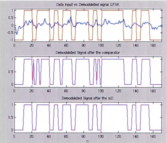
(51) 53 rate. The <lecision algorithm implementation an<l the lO\v pass filler <lesihrn are shO\m in Appen<lix l. Tu evaluate the impact uf the <lecisiun algurithm, a cumparatur after the lO\v pass filler vva.s implemente<l too. Figure 5.7 shows the <lemu<lulatur sih'nals. In the lirst plut the data input is plutte<l versus the GFSK <lemo<lulate<l sihrnal. In the next plut, the GFSK <lemu<lulate<l sie,rnal al'ter the rnmparator is shown. Finally, the GFSK <lemo<lulate<l sie,rnal after the <lecision algurithm is shown.. 0.5. o -0.5 -1 .___. o. __...J_ _ _ ____. _ ____,__ ___._ _ _......L._. 20. 40. 60. ___.__ _....L..._ _...J......__J. 100. 80. 120. 140. 160. 140. 160. Demodulated Signa! after the comparator. 0.5. o o. 20. 40. 60. 100. 80. 120. Demodulated Signa! after the laD. 0.5. o o. 20. 40. 60. 100. 80. 120. n. Figrne5. 7 a) GFSK demodulated signa] and data input. b) GFSK demodulated signal afl.er the comparaloL c) GFSK demo<lulaled signa! afler laD. Fura GFSK <lemu<lulatur, the receive<l signal nee<ls tu be syndu-unize<l <lue tu the <lday pru<luce<l by the Gaussian lilter. lJp to this point, the simulation has heen rnnsi<lere<l noisdess. That's because there are notable <lifferences betv.een the signal after the rnmparatur an<l alter the laD. Tu ubtain the enur perfunnam:e uf the GFSK <lemu<lulatur, lhe mu<lulate<l signal vvas passe<l thruugh an A WGN chaimel. This simulatiun is presente<l in the nexl sediun..

(52) 54 5.1.4 TRANSMISSION THROllGH AN ADDITIVE WHITE GAllSSIAN NOISE (A WGN). ERROR PERFORMANCE (BER) Figure 5.8 shmvs the GFSK demodulatur signals 'vvith added noise. This simulation presented considered a Eb/No = 4dB.. Data Input vs Demodulated signa! GFSK 0.5. o -0 .5. -1. L - - - - - - L - - - - - - 1 . - ---L..--. o. 20. 40. 60. - 1 . - - -..J..._--J...._-----L_ ____¡____J. 100. 80. 120. 140. 160. Demodulated Signa! after the comparator. 0.5. _ ____.___ ____.____....___.,___. o...___ o. __._. ____.. 20. 40. 60. 100. 80. ____.. ____._____,. 120. 140. 160. 120. 140. 160. Demodulated Signa! after the laD. 0.5. o o. 20. 40. 60. 100. 80. n. Figure5.8 GFSK signals with noise. a) GFSK demodulated signa! and data input, b) GFSK demodulated sie,'lml after the comparator, l.:) GFSK demodulated signa! after laD. I lere, the impact uf the laD is evident. The signa! after the comparator has severa! errors. The perfonna1Ke after the laD improves redul:ing the number uf eITurs per bit as l:UI1 be seen in the figure 5.8. In order to a11alyze the error perfonna11ce uf the demodulator, a simulation of a large pseudo ra11dom seque1Ke al different values uf Eb/No over a11 A WGN cha1111el was done. The perfo1111a1Ke uf the GFSK demodulator with a11 laD algorithm is presented in Figure 5.9 'v\Ílh the theoretical FSK non-coherent demodulator a11d the theoretical FSK coherent demodulation [5]..

(53) 55 o ~-~-~-~-~---,-----,-----,----,-------,--,----,---~---,. 1. ........ .0 1. ~ -3. + - - - - - - - - - - - - - - - - - - -__::,__~ -----. -""'-- - - 1. GJ. D.. -5. -+--------------------------------<. -6 - ' - - - - - - - - - - - - - - - - - - - - - - - - - - - ~ EbNo. - - FSK coherent theory. - - FSK non-coherent theory (GFSK with IaD). Figure5.9 GFSK \\ ith laD Probability ol' error compared wilh FSK 11011-coherenl demodulalion and ,,ith FSK coherent demodulation.. As can be observed in the rnrves, the perfonnam:e uf a GFSK nun-cuherent demudulalion is impruved with the laD decision algorithm. This impruve, allovvs the GFSK nun-cuherent demodulation 'vvith laD to have at almost equal the perfonnance of a FSK cuherent demodulalion. There is the importance of having a decision algorithm.. 5.2 MATLAB SIMULATION OF A GSFK MODEM AT 2 MHZ (ONE BLUETOOTH CHANNEL) ln this section, a 2 Ml lz GfSK Modem applied to I31uetooth is presented. Acrnrding to l3luetooth standard requirements, the modem has been simulated as follows [6]: • • • • •. The modulation index h must vary betv.een 0.28 and 0.35, The bit rate of one chmmel is 1Mbps, The channel bamhvidth is equal to l MI lz, The Gaussia11 Filler para111eter BT-0.5 and The sample frequency is 1~ -so MI Iz.. ln order to define the modulation factor, we rev.rite here the expression (4.1.2 ):. D..f=li•jb. Substituting the values of the Bluetooth sta11dard, the ti/ Cilll vary from 0.28 tu 0.35 Mllz. Su, the frequency fi, bet'v\een the central frequency L and the markers fi ami 1~i can vary from 0.14 to.

(54) 56 0.175 MHz. In this simulation a modulation index h=0.32 is considered, then the fd=l60 k..Hz. lt represents that fn:quencies f1 and fo will be multiples of 10 kllz. Then the sine table must generate frequencies in multiples uf 1Okllz. lt origins a length table uf:. f. 80MHz. N =-' = =8000 Ísiep IOKH-::,. Table shmvs the frequency selection for different central frequencies with an index moJulation uf h=0.32 anJ for an integer k Jelays. Table5.2 GFSK parameters with h=0.32. FREQUENCY fREQUENCY NUMBEROF (fe) DELAY SAMPLES WlTH Fs= 801\ffiz 800000 1000000 1250000 2000000 2500000 4000000 20000000. The channel to be simulated modulations are:. 3200000 4000000 5000000 8000000 10000000 16000000 80000000. \-\-ill. 25 20 16 10 8 5 1. h=0.32 Fl. FO. 960000 1160000 1410000 2160000 2660000 4160000 20160000. 640000 840000 1090000 1840000 2340000 3840000 19840000. be cenlered al lMllz. Then the two frequencies uf FSK. J; = 1160000 H: J~ = 840000 II: The moJem \-Vas simulated \-\-Íth the prol:,rrai11s presented in Appendix A. As we mentioned, these programs responds at the parameters f1. fu, t and fb. So with the founded parameters and thc prograins in Matlab is easy lo obtain a simulation. In the next sections the results are presenled..

(55) 57. 5.2.1 MODULATION The first module to be considered is the modulator. The two frequencies of FSK modulations are then: J; = 1160000 Hz. J11 = 840000 Hz Then, in order to define the steps for the sine table, the following table can be used:. k. = 1. f •N f. k= f •N. =. 1160000 • 80000. =. I 16. =. 84. 80000000 =. I. 840000• 80000. 80000000. Ali these paran1eters were included in the Matlab progran1 for the modem; the simulation results for the PSK 2 MHz Modem are sho\\ln in figure 5.1 O.. 15. 0.6. o D. 41D. BlJ. 41D. BlJ. 1cm. 1DJ. ICIIJ. 1DJ. as D. ~5 -1 D. IDI. n. Figure5. l O Bluetooth GFSK modulation. The pluts already indude the Gaussian filler fur lhe GFSK mudem. 1luvvever lhe effed uf lhe Gaussian filler is nul dearly in lhe pluts; lhis effed l:an be beller analyze<l using a Pu'A'er.