Associative learning on imbalanced environments: An empirical study

Texto completo

(1)Associative learning on imbalanced environments: An empirical study L. Cleofas-Sáncheza , J.S. Sáncheza,, V. Garcı́ab , R.M. Valdovinosc a. Institute of New Imaging Technologies, Department of Computer Languages and Systems, Universitat Jaume I, Castelló de la Plana, Spain E-mail: [email protected], [email protected] b División Multidisciplinaria de Ciudad Universitaria, Universidad Autónoma de Ciudad Juárez, Ciudad Juárez, Chihuahua, Mexico E-mail: [email protected] c School of Engineering, Universidad Autónoma del Estado de México, Toluca, Mexico E-mail: li [email protected]. Abstract Associative memories have emerged as a powerful computational neural network model for several pattern classification problems. Like most traditional classifiers, these models assume that the classes share similar prior probabilities. However, in many real-life applications the ratios of prior probabilities between classes are extremely skewed. Although the literature has provided numerous studies that examine the performance degradation of renowned classifiers on different imbalanced scenarios, so far this effect has not been supported by a thorough empirical study in the context of associative memories. In this paper, we fix our attention on the applicability of the associative neural networks to the classification of imbalanced data. The key questions here addressed are whether these models perform better, the same or worse than other popular classifiers, how the level of imbalance affects their performance, and whether distinct resampling strategies produce a different impact on the associative memories. In order to answer these questions and gain further insight into the feasibility and efficiency of the associative memories, a large-scale experimental evaluation with 31 databases, seven classification models and four resampling algorithms is carried out here, along with a non-parametric statistical test to discover any significant differences between each pair of classifiers. Keywords: Associative memory, Class imbalance, Resampling. Preprint submitted to Expert Systems with Applications. May 27, 2016.

(2) 1. Introduction Associative memories have been an active research area in pattern recognition and neuroscience for over 50 years (Palm, 2013). Although typical applications of these connectionist models include image recognition and recovery, data analysis, control, inference and prediction (Danilo et al., 2015; Kareem and Jantan, 2011; Lou and Cui, 2007; Mu et al., 2006; Nazari et al., 2014; Štanclová and Zavoral, 2005), the associative memories have lately emerged as useful classifiers for a large variety of problems in data mining and computational intelligence (AldapePérez et al., 2012, 2015; Sharma et al., 2008; Uriarte-Arcia et al., 2014). From a practical point of view, classification refers to the assignment of a finite set of samples to predefined classes based on a number of observed variables or attributes. The effective design of classifiers is a complex task where the underlying quality of data becomes critical to further achieve accurate classifications. Besides other factors, the performance of classifiers strongly depends on the adequacy of the data in terms of several intrinsic characteristics such as number of examples, relevance of the attributes, class distribution and completeness of data. In particular, a very common situation in real-life classification problems is to find data sets where the amount of examples available for one class is quite different from that of the other classes. This significant difference in the size of the classes is usually known as class imbalance, and it has been observed that most traditional classifiers perform poorly on the minority class because they assume an even class distribution and equal misclassification costs (Japkowicz and Stephen, 2002). Examples of applications with skewed class distributions can be found in many different areas ranging from bioinformatics and medicine to finance, network security and text mining. For instance, in credit risk and bankruptcy prediction, the number of observations in the class of defaulters is much smaller than the number of cases belonging to the class of non-defaulters (Kim et al., 2015). Gene expression microarray analysis for cancer classification shows significant differences between the number of cancerous and healthy tissue samples (Blagus and Lusa, 2010). Web spam detection exhibits an asymmetric distribution between legitimate and spam pages (Fdez-Glez et al., 2015). Within this context, the major research line has traditionally been directed to the development of techniques to tackle the class imbalance at both algorithmic and data levels (He and Garcia, 2009; He and Ma, 2013; López et al., 2013). The methods at the algorithmic level modify the existing learning models for biasing the discrimination process towards the minority class; the data level solutions consist of a preprocessing step to resample the original data set, either by over2.

(3) sampling the minority class and/or under-sampling the majority class, until the classes are approximately equally represented. In general, the resampling strategies have been the most widely used because they are independent of the classifier and can be easily implemented for any problem (Cao et al., 2014; Garcı́a et al., 2012). Over the last years, however, research on this topic has also put the emphasis on studying the effect of imbalance together with other data complexity characteristics such as overlapping, small disjuncts and noisy data (He et al., 2015; López et al., 2013; Napierala et al., 2010; Prati et al., 2004; Stefanowski, 2013). Another critical subject that has attracted increasing interest in the scientific community is how to assess the performance of a classification model in the presence of imbalanced data sets because most common metrics (e.g., accuracy and error rates) strongly depend on the class distribution and assume equal misclassification costs, which may lead to distorted conclusions (He and Garcia, 2009; Menardi and Torelli, 2014). In addition to the aforementioned questions, research has also placed its attention on evaluating and comparing the performance of competing classifiers (Brown and Mues, 2012; Kwon and Sim, 2013; López et al., 2013; Liu et al., 2011; Seiffert et al., 2014), but many of these works do not take into consideration the impact of different levels of imbalance on the performance of each particular classification model, neither the implications of using this jointly with one resampling technique or another. While research in class imbalance has mainly concentrated on well-known classifiers such as support vector machines (Akbani et al., 2004; Hwang et al., 2011; Liu et al., 2011; Maldonado and López, 2014; Yu et al., 2015), kernel methods (Hong et al., 2007; Maratea et al., 2014), k-nearest neighbors (Dubey and Pudi, 2013), decision trees (Kang and Ramamohanarao, 2014) and multiple classifier systems (Dı́ez-Pastor et al., 2015; Galar et al., 2012; Krawczyk et al., 2014; Park and Ghosh, 2014), very few theoretical or empirical analyses have been done so far to thoroughly establish the performance of associative memories when learning from class imbalanced data. Therefore, the present study intends to extend the very preliminary existing works (Cleofas-Sánchez et al., 2013, 2014) by increasing the scope and detail at which a type of associative memory networks (the hybrid associative classifier with translation) performs in the framework of class imbalance. We believe that the extensive experimental analysis here carried out will allow to gain a deeper insight into the feasibility and efficiency of these associative memories and help researchers and practitioners to build effective associative learning models and develop techniques based on associative learning 3.

(4) to handle the class imbalance problem. To sum up, the purpose of this paper is three-fold: • To explore the performance of the hybrid associative memory with translation and compare this against other popular classification methods of different nature; • to investigate how the imbalance ratio affects the performance of these associative memories; and • to analyze the impact of several resampling strategies on the performance of the associative neural network. The rest of this paper is organized as follows. Section 2 introduces the bases of the associative memory neural networks and in particular, of the hybrid associative classifier with translation. Section 3 briefly describes four resampling methods to deal with the imbalance problem, which will be further used in the experiments. The experimental set-up and databases are presented in Section 4, while the results and statistical tests are discussed in Section 5. Finally, Section 6 remarks the main conclusions and outlines some avenues for future research. 2. Associative memories The associative memory is an early type of artificial neural network that takes the form of a matrix M generated from a finite set of p previously known associations, which is called fundamental set {(xµ , yµ ) | µ = 1, 2, . . . , p}, where xµ are the fundamental input patterns of dimension n and yµ are the the fundamental output patterns of dimension m. Then, xµj and yjµ denote the j-th component of an input pattern xµ and of an output pattern yµ , respectively. Functionality of the associative memories is accomplished in two phases: learning and recall. The learning process consists of building a matrix M with a value for each association (xk , yk ). In the recall phase, an output vector y is obtained from the associative memory; this vector is the most similar to the input vector x. These memories have the capability of storing huge amounts of data that allow to recover the input examples with low computational efforts. The associative memories can be of two types (Aldape-Pérez et al., 2012): heteroassociative (e.g., linear associator) and autoassociative (e.g., Hopfield network). The heteroassociative memories relates input patterns with output patterns 4.

(5) of distinct nature and formats (xµ ̸= yµ ), while the autoassociative memories are a particular case where xµ = yµ and n = m. Some of the most widely-studied models of associative memories are lernmatrix (Steinbuch, 1961), the linear associator (Anderson, 1972; Kohonen, 1972), the Hopfield network (Hopfield, 1982), the bidirectional associative memory (Kosko, 1987), and the morphological associative memory (Ritter et al., 1998). The popularity of these models comes from their capability of storing huge amounts of data that allow to properly recover the most similar patterns given an input vector with low computational efforts, but they have some difficulties to discriminate between classes. 2.1. The hybrid associative classifier with translation With the aim of extending the applicability of classical associative memories to classification tasks, Santiago (2003) introduced the hybrid associative classifier with translation (HACT), which is based on the learning phase of the linear associator and the recall phase of the lernmatrix. The learning phase of the linear associator comprises two steps: 1. For each association (xµ , yµ ), compute the matrix (yµ )·(xµ )T , where (xµ )T is the transpose input vector. ∑ 2. Sum the p matrices to obtain the memory M = pµ=1 (yµ ) · (xµ )T , being ∑ mi,j = pµ=1 (yiµ )(xµj )T its (i, j)-th component. On the other hand, the recall phase of the lernmatrix consists of finding the class of an input pattern xµ , that is, to find the components of the vector yµ associated to xµ , whose i-th component is calculated according to the following expression: [∑ ] { ∑n n µ p µ 1 if m x = max m x i,j j h,j j h=1 j=i j=i yiµ = (1) 0 otherwise Note that if xµ belongs to class c, this expression leads to an m-dimensional vector with all components equal to zero except for the c-th component whose value is equal to 1. In addition, the HACT model incorporates the translation of the axes to a new origin located at the centroid of the fundamental input patterns. Let A = {xµ | µ = 1, 2, . . . , p} be a set of n-dimensional fundamental input patterns that belong to. 5.

(6) Algorithm 1 HACT – learning phase s←0 for all xµ ∈ A do s ← s + xµ end for x ← s/p {x is the new origin of the coordinates axes}. for all xµ ∈ A do x̂µ ← xµ − x {Translate the input patterns to the new coordinates axes} c←1 {Assign an output vector of size m to patterns that belong to class c} while c ≤ m do if class(x̂µ ) = c then ycµ = 1 else ycµ = 0 end if end while end for M ← 0 {Apply the learning phase of the linear associator} for all (x̂µ , yµ ) do M ← M + (yµ ) · (x̂µ )T end for. m classes, then the learning phase of HACT to construct the matrix M consists in the steps of Algorithm 1. Once the matrix M has been generated, the classification of a new input pattern x consists of applying the recovery phase of lernmatrix according to expression 1. 3. Resampling methods to handle class imbalance Much research has been conducted to tackle the class imbalance problem by applying different resampling strategies that change the class distribution of the data set (Yang et al., 2011). This can be done by either over-sampling the minority class or under-sampling the majority class until both classes are approximately equally represented. Despite their advantages and popularity, several shortcomings remain associated with both these strategies because they artificially alter the prior class probabilities (Barandela et al., 2004): whilst under-sampling may result in throwing away potentially useful information about the majority class and perturbing the a priori probability of the training set (Dal Pozzolo et al., 2015), 6.

(7) over-sampling worsens the computational burden of most classifiers, may increase the likelihood of overfitting and introduce noise that could result in a loss of performance. 3.1. Over-sampling The simplest method to increase the size of the minority class corresponds to random over-sampling (ROS), which balances the class distribution through the random replication of minority class examples. Although this method appears to be quite effective without adding new information into the data set, it may increase the likelihood of overfitting because it makes exact copies of the minority class examples. In order to avoid overfitting, Chawla et al. (2002) proposed the Synthetic Minority Oversampling TEchnique (SMOTE) to up-size the minority class. Instead of merely replicating examples, this algorithm generates artificial examples of the minority class by interpolating existing instances that lie close together. It first finds the k positive nearest neighbors for each minority class example and then, the synthetic examples are generated in the direction of some or all of those nearest neighbors. SMOTE allows the classifier to build larger decision regions that contain nearby examples of the minority class. Depending upon the amount of over-sampling required, a certain number of examples from the k nearest neighbors are randomly chosen. 3.2. Under-sampling Random under-sampling (RUS) aims at balancing the data set through the random removal of examples that belong to the over-sized class. Despite important information can be lost when examples are discarded at random, it has empirically been shown to be one of the most effective resampling methods. Unlike the random approach, other under-sampling methods are based on a deterministic selection of the examples to be eliminated. For instance, Laurikkala (2001) introduced the Neighborhood CLeaning rule (NCL), which uses the Wilson’s editing algorithm (Wilson, 1972) to remove only the majority class cases that border the minority class examples, assuming that they are noise. 4. Experimental set-up With the aim of evaluating the performance of the HACT model on imbalanced domains, we have carried out a series of experiments on a large collection of imbalanced data sets using four resampling algorithms (ROS, SMOTE, RUS, 7.

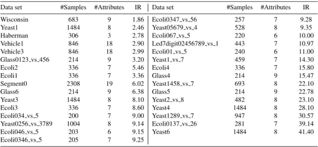
(8) and NCL) to preprocess the original data sets and seven classifiers implemented with the default parameter settings given by the WEKA toolkit (Hall et al., 2009): the Bayes network (BNet), a multilayer perceptron network with backpropagation (MLP), a normalized Gaussian radial basis function (RBF), a support vector machine with a linear kernel(SVM), a pruned decision tree (C4.5), the nearest neighbor with generalization (NNge), and the voted perceptron (VP). Note that we have chosen classifiers of different nature and complexity in order to draw meaningful conclusions, including four neural networks (BNet, MLP, RBF, VP), a linear classifier (SVM), a decision tree (C4.5), and an instance-based learner (NNge). 4.1. Data sets The experimental set-up has been designed following the common practice (Akbani et al., 2004; Barua et al., 2014; Dı́ez-Pastor et al., 2015; Galar et al., 2013; López et al., 2012, 2013; Yu et al., 2013, 2015), which consists of generating skewed data sets with different levels of class imbalance. In particular, the scheme proposed in the literature is to transform multi-class data sets by combining several original classes to shape the majority and minority classes. For instance, Glass0123 vs 456 is an imbalanced version of Glass database where the classes 0, 1, 2 and 3 have been combined to form a unique minority class and the original classes 4, 5 and 6 have been joined to represent the majority class. Similarly, Glass6 has been created by leaving the original class 6 as the minority class and merging the rest of the classes into a single majority class. The results are based on 31 imbalanced data sets taken from the KEEL Data Set Repository (Alcalá-Fdez et al., 2011), whose main characteristics are summarized in Table 1. These data sets have been divided into two groups according to their imbalance ratio (IR), that is, the ratio of the majority class size to the minority class size. A first group comprises data sets with a low/moderate imbalance ratio (IR < 10), while the second category gathers the strongly imbalanced databases (IR ≥ 10). The five-fold cross-validation method has been adopted for the experimental design because it seems to be the best estimator of classification performance compared to other methods, such as bootstrap with a high computational cost or re-substitution with a biased behavior. Each original data set has randomly been divided into five stratified parts of of size n/5 (where n denotes the total number of samples in the data set); for each fold, four blocks have been pooled as the training set, and the remaining portion has been used as an independent test set.. 8.

(9) Table 1: Data sets used in the experiments Data set Wisconsin Yeast1 Haberman Vehicle1 Vehicle3 Glass0123 vs 456 Ecoli2 Ecoli1 Segment0 Glass6 Yeast3 Ecoli3 Ecoli034 vs 5 Yeast0256 vs 3789 Ecoli046 vs 5 Ecoli0346 vs 5. #Samples. #Attributes. IR. 683 1484 306 846 846 214 336 336 2308 214 1484 336 200 1004 203 205. 9 8 3 18 18 9 7 7 19 9 8 7 7 8 6 7. 1.86 2.46 2.78 2.90 2.99 3.20 5.46 3.36 6.02 6.38 8.10 8.60 9.00 9.14 9.15 9.25. Data set Ecoli0347 vs 56 Yeast05679 vs 4 Ecoli067 vs 5 Led7digit02456789 vs 1 Ecoli01 vs 5 Yeast1 vs 7 Ecoli4 Glass4 Yeast1458 vs 7 Glass5 Yeast2 vs 8 Yeast4 Yeast1289 vs 7 Ecoli0137 vs 26 Yeast6. #Samples. #Attributes. IR. 257 528 220 443 240 459 336 214 693 214 482 1484 947 281 1484. 7 8 6 7 6 7 7 9 8 9 8 8 8 7 8. 9.28 9.35 10.00 10.97 11.00 14.30 15.80 15.47 22.10 22.78 23.10 28.10 30.57 39.14 41.40. The classification models have been applied to the sets preprocessed by the resampling strategies and also to each original training set, which can be deemed as a baseline for comparison. The results from classifying the test samples have been averaged across the five runs and then evaluated for significant differences using the non-parametric Wilcoxon signed-rank test (Demšar, 2006). 4.2. Evaluation criteria Although the accuracy (and its counterpart, the error rate) is the most commonly used metric to evaluate the performance of classification systems, it has been demonstrated not to be appropriate when the prior class probabilities are very different because it does not consider misclassification costs, is strongly biased to favor the majority class, and is very sensitive to class skews (Daskalaki et al., 2006; Japkowicz, 2013). Therefore, the effectiveness of classifiers in imbalanced domains has traditionally been evaluated by using other criteria, such as precision, area under the ROC curve, F -measure, and geometric mean of accuracies. In this paper, the geometric mean of accuracies has been chosen because it represents a good trade-off between the rates measured separately on each class. Gmean =. √. T P rate · T N rate. (2). where T P rate and T N rate denote the accuracy on the minority and majority classes, respectively. 9.

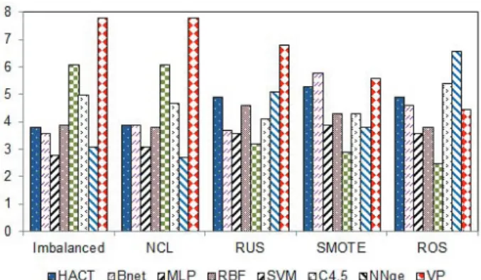
(10) 5. Experimental results and discussion The purpose of these experiments is three-fold: (i) to evaluate the performance of the HACT model in comparison to that of other classifiers when the data set is imbalanced; (ii) to find out whether there exist differences in its behavior depending on the imbalance ratio; and (iii) to determine how the application of resampling strategies affects the effectiveness of the HACT classifier. At this point, we believe that the degree of difficulty of classification of imbalanced data sets depends on their class imbalance ratio. This hypothesis can be extended to the resampling techniques and to the different classifiers. This is the reason why the experiments and analysis have been performed according to two levels of imbalance. The Gmean results have been tested for statistically significant differences by means of non-parametric tests, which are generally preferred over the parametric methods because the usual assumptions of independence, normality and homogeneity of variance are often violated due to the non-parametric nature of the problems (Demšar, 2006). Both pairwise and multiple comparisons have been used in this paper. First, we have computed the Friedman’s ranking of the classifiers for each resampling strategy and each data set independently according to the Gmean results: as there are eight competing classifiers, the ranks for each data set go from 1 (best) to 8 (worst); in case of ties, average ranks are assigned. Then the average rank of each model across all data sets has been calculated. Afterwards, the Wilcoxon’s paired signed-rank test has been used to find out statistically significant differences between each pair of classifiers for two levels of significance (α = 0.10 and α = 0.05). This statistic ranks the differences in performances of two algorithms for each data set, ignoring the signs, and compares the ranks for the positive and the negative differences. 5.1. Results on databases with low/moderate imbalance The detailed results over each problem are given in the Appendix. Here the Friedman’s average ranks for the eight classification models have been plotted in Figure 1. For the original training sets, the MLP and NNge classifiers arise as the algorithms with the lowest rankings, that is, the highest performance in average; when using the under-sampling strategies to balance the data sets, it seems that the best classifiers depend on the particular algorithm used. With the over-sampling techniques, SVM yields the lowest rankings. Despite the HACT model has never obtained the lowest average ranks, it is worth noting that their rankings are not too far from those of the best classifiers. 10.

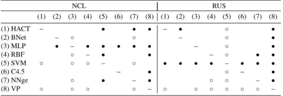
(11) Figure 1: Friedman’s average ranks for databases with low/moderate imbalance. Tables 2–4 report the Wilcoxon’s test for the data sets with a low/moderate imbalance ratio. The upper diagonal half of each table corresponds to a significance level of α = 0.10 (10% or less chance), whereas the lower diagonal half is for α = 0.05. The symbol “•” indicates that the classifier in the row significantly outperforms the classifier in the column, and the symbol “◦” means that the classifier in the column performs significantly better than the classifier in the row. Table 2: Wilcoxon’s statistic for the original training sets with low/moderate imbalance (1) (2) (1) HACT (2) BNet (3) MLP (4) RBF (5) SVM (6) C4.5 (7) NNge (8) VP. (3) (4). – – ◦. ◦. ◦. ◦. o – ◦ ◦ ◦. • – ◦. ◦. ◦. (5) (6) • • • • – • • ◦. (7) (8). • ◦ – • ◦. ◦ ◦ – ◦. • • • • • • • –. Results in Table 2 show that the HACT model performs significantly better than the SVM and VP classifiers at both significance levels when the imbalanced training set has not been preprocessed. In this scenario, the performance of the MLP neural network is significantly better than that of the RBF, SVM, C4.5 and VP algorithms, while NNge outperforms SVM, C4.5 and VP. Although both MLP and NNge appears to be the best alternatives when data sets present a low or moderate imbalance ratio, it has to be noted that the differences between these 11.

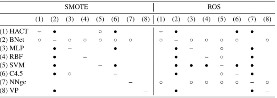
(12) two classifiers and HACT are not statistically significant and their computational cost is high when the data set size is large. In Tables 3–4, one can observe that the behavior of HACT varies considerably depending on whether the data sets are under- or over-sampled: while the removal of majority class examples seems not to change its performance significantly, the over-sampling algorithms degrade the effectiveness of the HACT classifier, especially with the SMOTE method (RBF, SVM and NNge perform significantly better than HACT for a significance level of α = 0.10). Table 3: Wilcoxon’s statistic for the under-sampled sets with low/moderate imbalance NCL (1) (1) HACT (2) BNet (3) MLP (4) RBF (5) SVM (6) C4.5 (7) NNge (8) VP. (2). (3). –. ◦ –. (4). RUS (5) (6). (7). (8). ◦ ◦ – ◦. • • • • • • • –. –. ◦ ◦. ◦. ◦ ◦ ◦. – ◦ ◦. • • • – • • ◦. • • ◦ – • ◦. (1) (2) (3) (4) (5). (6). ◦. –. • •. – – ◦. •. • – •. (7) (8). ◦ –. • –. ◦. ◦. ◦ ◦. ◦. ◦ ◦. ◦. – ◦. • • • • • • –. Table 4: Wilcoxon’s statistic for the over-sampled sets with low/moderate imbalance SMOTE (1) (1) HACT – (2) BNet (3) MLP (4) RBF (5) SVM • (6) C4.5 (7) NNge (8) VP. (2). (3). – • • • • •. ◦ –. (4) ◦ ◦. ROS (5) (6) ◦ ◦ ◦. (7) ◦ ◦. (8). – – ◦. ◦. • – – ◦. • • • • • –. (1) (2) (3) (4) (5) – ◦ – ◦ ◦ ◦ • – • – ◦ • • • – ◦ ◦ ◦ ◦ ◦ ◦ ◦ ◦ ◦. (6) • • • – ◦. (7) (8) • • • • • • • – –. The three values in the cells of Table 5 show how many times the method of the column has been significantly-better/same/significantly-worse, with a significance level of α = 0.05, for the databases with a low/moderate imbalance rate. As can be observed, the MLP neural network performs the best with both the imbalanced sets and the under-sampled sets, while the SVM appears to outperform the other 12.

(13) classifiers when the data sets have been over-sized. The HACT model does not present significant differences with the best approaches when using the original training set and the sets under-sampled with the NCL algorithm and therefore, it can considered as one of the best alternatives. However, the use of SMOTE and ROS seems to produce some degradation on the performance of the HACT classifier. Table 5: Summary of the Wilcoxon’s statistic for the sets with low/moderate imbalance. Original NCL RUS SMOTE ROS. HACT. Bnet. MLP. RBF. SVM. C4.5. NNge. VP. 2/5/0 1/6/0 1/5/1 0/6/1 1/5/1. 2/5/0 2/5/0 1/6/0 0/2/5 1/3/3. 4/3/0 2/4/1 3/4/0 2/5/0 3/4/0 1/4/2 1/6/0 2/5/0 3/4/0 3/3/1. 1/0/6 1/1/5 4/3/0 3/4/0 6/1/0. 2/3/2 2/3/2 1/5/0 1/6/0 1/4/3. 3/4/0 3/4/0 1/4/2 2/5/0 0/1/6. 0/0/7 0/0/7 0/0/7 0/4/3 0/6/1. 5.2. Results on databases with high imbalance Figure 2 shows the Friedman’s average ranks for the eight classification models under a high imbalance ratio. For the imbalanced sets, the lowest rankings correspond to the MLP, Bnet and HACT neural networks. Although there is not a best performing classifier with the resampling algorithms, it seems that the HACT model is one of the approaches with lower rankings independently of the technique used.. Figure 2: Friedman’s average ranks for strongly imbalanced databases. 13.

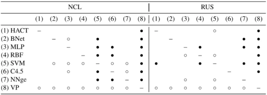
(14) The Wilcoxon’s test reported in Table 6 reveals that the performance of HACT is significantly better than that of SVM, NNge and VP at both significance levels when the original training sets are strongly imbalanced. In this sense, its behavior seems to be similar to that of MLP since this classifier performs significantly better than RBF, SVM, C4.5, NNge and VP. Table 6: Wilcoxon’s statistic for the original training sets with high imbalance (1) (2) (1) HACT (2) BNet (3) MLP (4) RBF (5) SVM (6) C4.5 (7) NNge (8) VP. (3) (4). • – ◦ ◦. • ◦. – ◦. ◦. ◦ ◦. ◦. – ◦ ◦ ◦ ◦ ◦. (5) (6) • • • • –. –. (7) (8). •. •. •. •. ◦ –. ◦. ◦. – ◦. • • • • • • • –. When the data sets with a high imbalance rate are under-sampled with the NCL algorithm, Table 7 shows that the HACT model achieves significantly better results than SVM and VP at a significance level of 0.05. The MLP neural network performs significantly better than BNet, RBF, SVM, NNge and VP, but we do not find statistically significant differences between the performance of MLP and that of HACT. In the case of random under-sampling, the SVM appears to be the best performing classifier since its Gmean results are significantly better than those of the remaining algorithms for α = 0.05. Nevertheless, the HACT neural network is still better than VP and is not significantly worse than the other classifiers. Table 7: Wilcoxon’s statistic for the under-sampled sets with high imbalance. (1) (1) HACT (2) BNet (3) MLP (4) RBF (5) SVM (6) C4.5 (7) NNge (8) VP. (2). NCL (3) (4). •. –. ◦. ◦ – ◦ ◦. ◦. ◦ ◦. – •. (5) (6). • – ◦. • • –. •. (7). (8). • ◦ •. •. ◦ –. ◦. •. – ◦. 14. • • • • –. RUS (1) (2) (3) (4) (5) –. • – –. • ◦. •. •. – •. ◦. ◦ ◦. ◦ ◦ ◦ ◦ – ◦ ◦ ◦. (6). • – ◦. (7) (8). • • – ◦. • • • • • • • –.

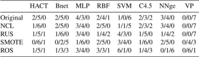
(15) On the other hand, when the training sets are over-sampled by means of the SMOTE method (see Table 8), it seems that no classifier performs significantly the best for any value of α. In this case, the BNet approach clearly corresponds to the worst model since its performance is significantly lower than that of any other classifier. With random over-sampling, the conclusions are similar to those drawn for the RUS algorithm, that is, the SVM seems to be the best performing method. However, in this scenario, the performance of HACT is statistically the same as that of the SVM and better than that of BNet and NNge. Table 8: Wilcoxon’s statistic for the over-sampled sets with high imbalance SMOTE. (1) HACT (2) BNet (3) MLP (4) RBF (5) SVM (6) C4.5 (7) NNge (8) VP. (1). (2). – ◦. • – • • • •. (3). (4). ◦ –. ◦. ROS (5) (6) ◦ ◦. • ◦ •. –. • –. (7). (8). (1) (2) (3) (4) (5) – ◦. ◦. – ◦. ◦. – •. –. • – • • • • •. ◦ –. ◦. •. – •. ◦. ◦. (6) • ◦. ◦ ◦ ◦ – ◦ ◦. • – ◦. (7) (8) • • • • • – •. ◦. ◦ –. Table 9 summarizes how many times the method of the column has been significantly-better/same/significantly-worse, with a significance level of α = 0.05, for the strongly imbalanced databases. In this case, the HACT model is among the best performing methods, especially with the original training set and the over-sampled sets. With the RUS algorithm, the SVM is clearly the best alternative because it has been significantly better than all the remaining classifiers. On the other hand, VP and Bnet appear to be the worst models: the former with the under-sampling techniques and the latter with the over-sampling algorithms. Table 9: Summary of the Wilcoxon’s statistic for the sets with high imbalance. Original NCL RUS SMOTE ROS. HACT. Bnet. MLP. RBF. SVM. C4.5. NNge. VP. 3/4/0 2/5/0 1/5/1 1/6/0 2/5/0. 2/5/0 0/6/1 0/6/1 0/1/6 0/1/6. 5/2/0 2/4/1 5/2/0 2/4/1 1/5/1 2/4/1 2/5/0 1/6/0 2/4/1 2/4/1. 1/1/5 0/3/4 7/0/0 1/6/0 5/2/0. 1/5/1 0/7/0 1/5/1 1/5/1 2/4/1. 2/3/2 2/4/1 1/4/2 0/7/0 0/1/6. 0/0/7 0/3/4 0/1/6 1/6/0 1/5/1. 15.

(16) 6. Conclusions and future work This paper intends to cover some questions on the application of the HACT neural network, which is a type of autoassociative memory, to problems characterized by skewed class distributions. Although earlier related works have given some insights into the effects of the class imbalance problem on this model, various interesting issues have not been studied in depth. Taking this into account, the main contributions can be summarized as follows: (i) we have empirically analyzed the performance of the HACT model in comparison to that of several standard classifiers; (ii) we have discussed the behavior of these classifiers as a function of the imbalance ratio; and (iii) we have studied how the use of different resampling techniques may affect the performance of the associative memory. Experimental results on a large collection of imbalanced data sets using four resampling techniques and seven different classifiers allow to remark some important findings that were not discussed in the few preliminary works: • When the imbalanced training set is not preprocessed by some resampling algorithm, the HACT model performs as well as the best classifier in most situations; • the superiority of HACT with respect to other classifiers is more significant in the case of strongly imbalanced data sets, both on the original (imbalanced) training sets and on the balanced sets; • the resampling strategies affect differently the performance of HACT depending on the imbalance ratio. Thus, when the imbalance is low or moderate, the over-sampling methods degrade the effectiveness of the HACT model considerably. However, with strongly imbalanced data, both underand over-sampling have given rise to very similar results. Despite the promising results in terms of the geometric mean of acuracies exhibited by the HACT model and supported by non-parametric statistical tests, there are still several interesting open research questions to work on. For instance, the present paper has focused on only the class imbalance problem, but a thorough and extensive analysis of the behavior of these neural networks when data sets are affected by multiple complexities deserves further future consideration. Another direction for extending this study is to investigate the applicability of the associative memories on imbalanced big data and data streams in a time-varying environment (concept change and concept drift), which are currently two hot topics in the literature related to expert and intelligent information systems. 16.

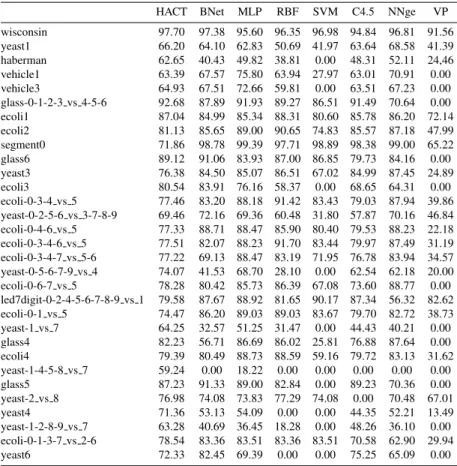
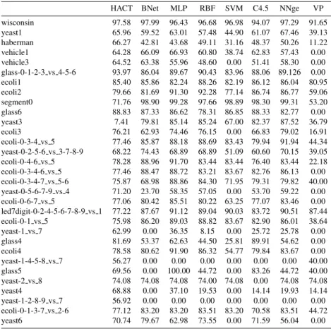
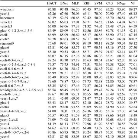
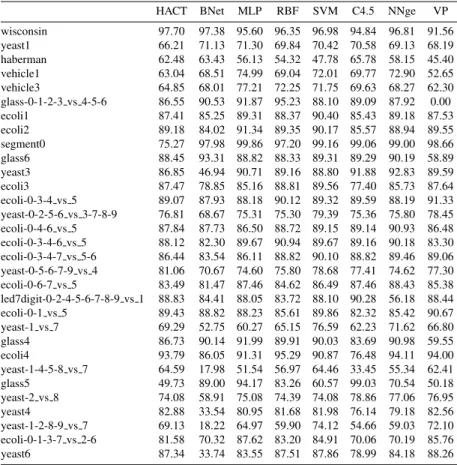
(17) Acknowledgment This work has partially been supported by the Mexican Science and Technology Council (CONACYT-Mexico) through the Postdoctoral Fellowship Program [232167], the Mexican PRODEP [DSA/103.5/15/7004], the Spanish Ministry of Economy [TIN2013-46522-P], and the Generalitat Valenciana [PROMETEOII/2014/062]. Appendix This appendix provides five tables with the Gmean results for the experimental analysis carried out in the present work. Table 10 contains the values for all the databases and classifiers achieved when using the imbalanced training sets, Table 11–14 shows the results with the sets preprocessed by NCL, random undersampling, SMOTE, and random over-sampling. References Akbani, R., Kwek, S., Japkowicz, N., 2004. Applying support vector machines to imbalanced datasets. In: 15th European Conference on Machine Learning. Pisa, Italy, pp. 39–50. Alcalá-Fdez, J., Fernández, A., Luengo, J., Derrac, J., Garcı́a, S., Sánchez, L., Herrera, F., 2011. KEEL data-mining software tool: Data set repository, integration of algorithms and experimental analysis framework. Journal of Multiple-Valued Logic and Soft Computing 17, 255–287. Aldape-Pérez, M., Yañez Márquez, C., Camacho-Nieto, O., Argüelles-Cruz, A. J., 2012. An associative memory approach to medical decision support systems. Computer Methods and Programs in Biomedicine 106 (3), 287–307. Aldape-Pérez, M., Yañez Márquez, C., Camacho-Nieto, O., López-Yáñez, I., Argüelles-Cruz, A. J., 2015. Collaborative learning based on associative models: Application to pattern classification in medical datasets. Computer in Human Behavior 51 (Part B), 771–779. Anderson, J. A., 1972. A simple neural network generating an interactive memory. Mathematical Bioscience 14, 197–220.. 17.

(18) Table 10: Geometric mean for the original data sets. wisconsin yeast1 haberman vehicle1 vehicle3 glass-0-1-2-3 vs 4-5-6 ecoli1 ecoli2 segment0 glass6 yeast3 ecoli3 ecoli-0-3-4 vs 5 yeast-0-2-5-6 vs 3-7-8-9 ecoli-0-4-6 vs 5 ecoli-0-3-4-6 vs 5 ecoli-0-3-4-7 vs 5-6 yeast-0-5-6-7-9 vs 4 ecoli-0-6-7 vs 5 led7digit-0-2-4-5-6-7-8-9 vs 1 ecoli-0-1 vs 5 yeast-1 vs 7 glass4 ecoli4 yeast-1-4-5-8 vs 7 glass5 yeast-2 vs 8 yeast4 yeast-1-2-8-9 vs 7 ecoli-0-1-3-7 vs 2-6 yeast6. HACT. BNet. MLP. RBF. SVM. C4.5. NNge. VP. 97.70 66.20 62.65 63.39 64.93 92.68 87.04 81.13 71.86 89.12 76.38 80.54 77.46 69.46 77.33 77.51 77.22 74.07 78.28 79.58 74.47 64.25 82.23 79.39 59.24 87.23 76.98 71.36 63.28 78.54 72.33. 97.38 95.60 64.10 62.83 40.43 49.82 67.57 75.80 67.51 72.66 87.89 91.93 84.99 85.34 85.65 89.00 98.78 99.39 91.06 83.93 84.50 85.07 83.91 76.16 83.20 88.18 72.16 69.36 88.71 88.47 82.07 88.23 69.13 88.47 41.53 68.70 80.42 85.73 87.67 88.92 86.20 89.03 32.57 51.25 56.71 86.69 80.49 88.73 0.00 18.22 91.33 89.00 74.08 73.83 53.13 54.09 40.69 36.45 83.36 83.51 82.45 69.39. 96.35 50.69 38.81 63.94 59.81 89.27 88.31 90.65 97.71 87.00 86.51 58.37 91.42 60.48 85.90 91.70 83.19 28.10 86.39 81.65 89.03 31.47 86.02 88.59 0.00 82.84 77.29 0.00 18.28 83.36 0.00. 96.98 41.97 0.00 27.97 0.00 86.51 80.60 74.83 98.89 86.85 67.02 0.00 83.43 31.80 80.40 83.44 71.95 0.00 67.08 90.17 83.67 0.00 25.81 59.16 0.00 0.00 74.08 0.00 0.00 83.51 0.00. 94.84 63.64 48.31 63.01 63.51 91.49 85.78 85.57 98.38 79.73 84.99 68.65 79.03 57.87 79.53 79.97 76.78 62.54 73.60 87.34 79.70 44.43 76.88 79.72 0.00 89.23 0.00 44.35 48.26 70.58 75.25. 96.81 68.58 52.11 70.91 67.23 70.64 86.20 87.18 99.00 84.16 87.45 64.31 87.94 70.16 88.23 87.49 83.94 62.18 88.77 56.32 82.72 40.21 87.64 83.13 0.00 70.36 70.48 52.21 36.10 62.90 65.09. 91.56 41.39 24,46 0.00 0.00 0.00 72.14 47.99 65.22 0.00 24.89 0.00 39.86 46.84 22.18 31.19 34.57 20.00 0.00 82.62 38.73 0.00 0.00 31.62 0.00 0.00 67.01 13.49 0.00 29.94 0.00. 18.

(19) Table 11: Geometric mean for the data sets preporcessed by NCL. wisconsin yeast1 haberman vehicle1 vehicle3 glass-0-1-2-3 vs 4-5-6 ecoli1 ecoli2 segment0 glass6 yeast3 ecoli3 ecoli-0-3-4 vs 5 yeast-0-2-5-6 vs 3-7-8-9 ecoli-0-4-6 vs 5 ecoli-0-3-4-6 vs 5 ecoli-0-3-4-7 vs 5-6 yeast-0-5-6-7-9 vs 4 ecoli-0-6-7 vs 5 led7digit-0-2-4-5-6-7-8-9 vs 1 ecoli-0-1 vs 5 yeast-1 vs 7 glass4 ecoli4 yeast-1-4-5-8 vs 7 glass5 yeast-2 vs 8 yeast4 yeast-1-2-8-9 vs 7 ecoli-0-1-3-7 vs 2-6 yeast6. HACT. BNet. 97.58 65.96 66.27 64.28 64.52 93.97 85.40 79.66 71.76 88.83 7.41 76.21 77.46 68.22 78.28 77.46 75.87 71.20 77.06 77.22 75.98 62.99 81.69 78.58 56.27 69.56 74.08 68.88 56.92 77.12 70.74. 97.99 96.43 59.52 63.01 42.81 43.68 66.09 66.93 63.38 55.96 86.04 89.67 85.86 82.24 81.69 91.30 98.90 99.28 87.33 86.62 79.81 85.14 62.93 74.46 85.87 88.18 74.43 68.89 88.96 91.70 88.47 88.72 68.98 88.86 23.70 58.35 80.42 85.51 87.67 91.12 86.20 89.03 0.00 36.35 53.37 62.63 80.62 91.90 0.00 0.00 0.00 100.00 74.08 74.08 0.00 37.10 0.00 0.00 83.20 83.20 79.67 62.98. MLP. 19. RBF. SVM. C4.5. 96.68 57.48 49.11 60.80 48.60 90.43 88.26 92.28 97.66 78.31 85.24 76.15 88.69 68.89 83.44 83.21 84.30 57.05 80.22 89.04 88.82 8.15 44.50 86.32 0.00 44.72 74.00 19.53 0.00 83.51 73.55. 96.98 44.90 31.16 38.74 0.00 83.96 82.19 77.14 98.89 86.85 67.00 0.00 83.43 51.09 83.44 83.67 71.95 0.00 63.25 90.03 83.67 0.00 25.81 54.77 0.00 0.00 74.08 0.00 0.00 83.20 0.00. 94.07 97.29 91.65 61.07 67.46 39.13 48.37 50.26 11.22 62.83 57.43 0.00 51.41 58.30 0.00 88.06 89.126 0.00 86.12 86.04 80.95 86.74 86.77 59.06 98.30 99.31 53.20 88.33 82.77 0.00 82.37 87.52 36.79 66.83 79.02 16.91 79.94 91.94 44.34 60.60 70.15 39.05 76.40 83.44 22.18 82.76 86.13 0.00 79.31 79.82 40.00 53.70 59.22 0.00 77.07 83.46 0.00 83.72 90.51 87.44 82.90 86.01 38.64 25.72 25.78 0.00 89.91 54.62 0.00 79.84 83.67 0.00 0.00 0.00 40.00 83.26 44.72 40.00 0.00 74.08 74.08 14.14 19.93 14.14 0.00 0.00 0.00 70.58 83.51 44.72 71.59 56.04 0.00. NNge. VP.

(20) Table 12: Geometric mean for the data sets preporcessed by RUS. wisconsin yeast1 haberman vehicle1 vehicle3 glass-0-1-2-3 vs 4-5-6 ecoli1 ecoli2 segment0 glass6 yeast3 ecoli3 ecoli-0-3-4 vs 5 yeast-0-2-5-6 vs 3-7-8-9 ecoli-0-4-6 vs 5 ecoli-0-3-4-6 vs 5 ecoli-0-3-4-7 vs 5-6 yeast-0-5-6-7-9 vs 4 ecoli-0-6-7 vs 5 led7digit-0-2-4-5-6-7-8-9 vs 1 ecoli-0-1 vs 5 yeast-1 vs 7 glass4 ecoli4 yeast-1-4-5-8 vs 7 glass5 yeast-2 vs 8 yeast4 yeast-1-2-8-9 vs 7 ecoli-0-1-3-7 vs 2-6 yeast6. HACT. BNet. MLP. RBF. SVM. C4.5. NNge. VP. 95.88 67.26 60.39 62.02 65.00 84.49 86.99 82.78 75.68 87.81 85.30 88.07 88.24 76.37 86.49 85.99 86.49 79.60 85.25 88.54 89.67 67.11 86.43 92.09 54.00 56.57 74.09 81.39 64.62 80.86 87.81. 97.48 96.20 67.60 70.06 52.25 60.68 66.03 77.01 68.06 77.33 89.09 91.77 85.09 86.69 89.63 88.57 99.01 99.02 92.06 85.77 90.53 90.48 87.15 82.76 93.30 87.19 75.75 74.91 84.20 88.47 91.21 81.30 80.05 92.98 78.87 75.40 85.91 87.46 88.45 85.83 88.78 85.71 45.40 69.07 86.17 88.79 90.60 93.55 0.00 53.36 90.52 91.59 74.08 65.45 81.13 77.50 42.03 68.96 60.95 70.74 87.40 83.03. 96.45 66.11 52.42 69.71 71.32 89.36 88.17 87.11 97.10 84.77 88.71 83.86 85.63 77.51 83.68 88.38 85.08 73.75 79.37 85.41 86.55 71.47 87.10 90.09 57.36 96.27 70.82 79.96 64.48 80.24 88.67. 97.36 70.00 50.90 74.52 74.02 85.86 86.88 88.63 98.11 90.54 89.39 86.36 88.54 78.36 88.62 87.07 89.90 78.38 86.24 89.47 88.34 77.73 86.21 95.48 59.90 90.79 72.53 81.70 73.89 80.87 88.69. 95.23 70.90 63.70 71.66 73.48 89.78 88.90 85.62 98.29 85.16 91.57 85.21 83.67 79.38 79.81 83.85 82.83 72.80 84.85 89.24 85.49 59.43 78.72 84.90 53.14 88.66 69.68 83.97 66.67 76.51 82.10. 95.96 67.40 56.54 64.94 67.38 91.13 87.12 86.94 99.34 87.32 92.14 80.92 82.20 72.60 81.77 85.74 82.07 73.00 86.24 73.80 82.68 67.12 85.90 93.20 57.30 84.84 63.44 78.58 62.47 78.86 80.03. 89.27 68.43 48.87 62.91 64.59 42.11 87.15 80.02 89.12 37.50 86.37 81.04 81.85 77.01 76.68 71.68 80.06 78.37 69.61 85.96 72.37 58.43 39.37 52.84 41.94 18.49 59.48 76.96 46.07 38.14 86.58. 20.

(21) Table 13: Geometric mean for the data sets preporcessed by SMOTE. wisconsin yeast1 haberman vehicle1 vehicle3 glass-0-1-2-3 vs 4-5-6 ecoli1 ecoli2 segment0 glass6 yeast3 ecoli3 ecoli-0-3-4 vs 5 yeast-0-2-5-6 vs 3-7-8-9 ecoli-0-4-6 vs 5 ecoli-0-3-4-6 vs 5 ecoli-0-3-4-7 vs 5-6 yeast-0-5-6-7-9 vs 4 ecoli-0-6-7 vs 5 led7digit-0-2-4-5-6-7-8-9 vs 1 ecoli-0-1 vs 5 yeast-1 vs 7 glass4 ecoli4 yeast-1-4-5-8 vs 7 glass5 yeast-2 vs 8 yeast4 yeast-1-2-8-9 vs 7 ecoli-0-1-3-7 vs 2-6 yeast6. HACT. BNet. MLP. RBF. SVM. C4.5. NNge. VP. 97.70 66.21 62.48 63.04 64.85 86.55 87.41 89.18 75.27 88.45 86.85 87.47 89.07 76.81 87.84 88.12 86.44 81.06 83.49 88.83 89.43 69.29 86.73 93.79 64.59 49.73 74.08 82.88 69.13 81.58 87.34. 97.38 95.60 71.13 71.30 63.43 56.13 68.51 74.99 68.01 77.21 90.53 91.87 85.25 89.31 84.02 91.34 97.98 99.86 93.31 88.82 46.94 90.71 78.85 85.16 87.93 88.18 68.67 75.31 87.73 86.50 82.30 89.67 83.54 86.11 70.67 74.60 81.47 87.46 84.41 88.05 88.82 88.23 52.75 60.27 90.14 91.99 86.05 91.31 17.98 51.54 89.00 94.17 58.91 75.08 33.54 80.95 18.22 64.97 70.32 87.62 33.74 83.55. 96.35 69.84 54.32 69.04 72.25 95.23 88.37 89.35 97.20 88.33 89.16 88.81 90.12 75.30 88.72 90.94 88.82 75.80 84.62 83.72 85.61 65.15 89.91 95.29 56.97 83.26 74.39 81.68 59.90 83.20 87.51. 96.98 70.42 47.78 72.01 71.75 88.10 90.40 90.17 99.16 89.31 88.80 89.56 89.32 79.39 89.15 89.67 90.10 78.68 86.49 88.10 89.86 76.59 90.03 90.87 64.46 60.57 74.08 81.98 74.12 84.91 87.86. 94.84 70.58 65.78 69.77 69.63 89.09 85.43 85.57 99.06 89.29 91.88 77.40 89.59 75.36 89.14 89.16 88.82 77.41 87.46 90.28 82.32 62.23 83.69 76.48 33.45 99.03 78.86 76.14 54.66 70.06 78.99. 96.81 69.13 58.15 72.90 68.27 87.92 89.18 88.94 99.00 90.19 92.83 85.73 88.19 75.80 90.93 90.18 89.46 74.62 88.43 56.18 85.42 71.62 90.98 94.11 55.34 70.54 77.06 79.18 59.03 70.19 84.18. 91.56 68.19 45.40 52.65 62.30 0.00 87.53 89.55 98.66 58.89 89.59 87.64 91.33 78.45 86.48 83.30 89.06 77.30 85.38 88.44 90.67 66.80 59.55 94.00 62.41 50.18 76.95 82.56 72.10 85.76 88.26. 21.

(22) Table 14: Geometric mean for the data sets preporcessed by ROS. wisconsin yeast1 haberman vehicle1 vehicle3 glass-0-1-2-3 vs 4-5-6 ecoli1 ecoli2 segment0 glass6 yeast3 ecoli3 ecoli-0-3-4 vs 5 yeast-0-2-5-6 vs 3-7-8-9 ecoli-0-4-6 vs 5 ecoli-0-3-4-6 vs 5 ecoli-0-3-4-7 vs 5-6 yeast-0-5-6-7-9 vs 4 ecoli-0-6-7 vs 5 led7digit-0-2-4-5-6-7-8-9 vs 1 ecoli-0-1 vs 5 yeast-1 vs 7 glass4 ecoli4 yeast-1-4-5-8 vs 7 glass5 yeast-2 vs 8 yeast4 yeast-1-2-8-9 vs 7 ecoli-0-1-3-7 vs 2-6 yeast6. HACT. BNet. MLP. RBF. SVM. C4.5. NNge. VP. 95.88 66.79 59.60 62.94 64.84 84.86 87.58 89.45 76.02 88.07 88.03 84.12 87.46 86.41 87.07 87.07 88.12 81.19 84.30 88.54 89.39 70.11 82.99 93.81 65.65 64.19 74.09 82.47 67.27 85.14 87.90. 97.80 96.19 71.77 69.94 61.39 55.67 67.94 81.29 67.99 81.35 89.48 91.77 86.30 85.70 86.84 91.13 93.17 99.70 89.19 85.77 89.59 91.32 82.25 86.12 88.94 87.43 75.09 74.35 76.40 83.26 84.71 88.72 81.21 89.45 66.06 72.85 85.73 90.80 88.31 87.48 83.29 88.02 54.28 74.28 47.93 89.22 83.13 91.16 41.71 33.80 44.72 89.23 52.90 72.70 57.13 74.85 49.08 48.14 44.64 81.50 74.56 79.62. 96.46 66.73 57.59 70.36 72.46 91.68 88.33 89.01 96.91 87.57 89.70 86.45 88.44 78.14 86.13 88.23 86.34 77.09 87.94 87.03 91.35 70.61 82.19 90.14 55.48 70.19 69.70 75.88 65.04 83.05 86.38. 97.28 70.63 55.95 76.00 73.23 88.68 89.78 90.96 99.16 88.32 88.76 85.95 89.32 79.41 88.89 89.42 90.31 78.68 86.49 87.97 89.00 77.38 90.27 90.58 64.61 93.69 74.08 80.45 73.29 85.09 87.73. 95.34 69.26 54.00 70.23 70.89 86.95 89.31 86.38 99.02 86.99 88.96 78.33 92.73 73.61 78.17 81.84 85.48 63.91 85.29 86.31 76.39 55.87 84.13 82.73 46.83 94.17 79.56 63.42 59.55 69.94 78.31. 96.58 65.33 47.10 58.01 52.90 82.32 85.31 83.97 97.54 74.00 89.59 74.33 85.14 68.25 88.23 87.49 83.75 53.70 89.21 89.01 82.72 44.24 44.36 77.21 25.75 44.72 70.63 36.74 47.68 70.58 50.62. 92.09 70.79 61.65 65.60 65.62 44.02 88.33 90.79 99.06 7.35 88.91 85.77 88.03 79.12 84.06 89.80 86.01 77.22 86.69 87.96 90.24 71.37 54.51 93.54 64.53 48.39 73.35 82.45 70.44 79.13 86.44. 22.

(23) Barandela, R., Valdovinos, R. M., Sánchez, J. S., Ferri, F. J., 2004. The imbalanced training sample problem: Under or over sampling? In: Fred, A., Caelli, T. M., Duin, R. P. W., Campilho, A. C., de Ridder, D. (Eds.), Structural, Syntactic, and Statistical Pattern Recognition. Vol. 3138 of Lecture Notes in Computer Science. Springer, pp. 806–814. Barua, S., Islam, M., Yao, X., Murase, K., 2014. MWMOTE–Majority weighted minority oversampling technique for imbalanced data set learning. IEEE Trans. on Knowledge and Data Engineering 26 (2), 405–425. Blagus, R., Lusa, L., 2010. Class prediction for high dimensaional classimbalanced data. BMC Bioinformatics 11 (523), 1–17. Brown, I., Mues, C., 2012. An experimental comparison of classification algorithms for imbalanced credit scoring data sets. Expert Systems with Applications 39 (3), 3446–3453. Cao, P., Zhao, D., Zaiane, O., 2014. Hybrid probabilistic sampling with random subspace for imbalanced data learning. Intelligent Data Analysis 18 (6), 1089– 1108. Chawla, N. V., Bowyer, K. W., Hall, L. O., Kegelmeyer, W. P., 2002. SMOTE: Synthetic minority over-sampling technique. Journal of Artifial Intelligence Research 16 (1), 321–357. Cleofas-Sánchez, L., Camacho-Nieto, O., Sánchez, J. S., Valdovinos-Rosas, R. M., 2014. Equilibrating the recognition of the minority class in the imbalance context. Applied Mathematics and Information Sciences 8 (1), 27–36. Cleofas-Sánchez, L., Garcı́a, V., Martı́n-Félez, R., Valdovinos, R. M., Sánchez, J. S., Camacho-Nieto, O., 2013. Hybrid associative memories for imbalanced data classification: An experimental study. In: Carrasco-Ochoa, J. A., Martı́nez-Trinidad, J. F., Rodrı́guez, J. S., di Baja, G. S. (Eds.), Pattern Recognition. Vol. 7914 of Lecture Notes in Computer Science. Springer, pp. 325–334. Dal Pozzolo, A., Caelen, O., Bontempi, G., 2015. When is undersampling effective in unbalanced classification tasks? In: Appice, A., Rodrigues, P. P., Santos Costa, V., Soares, C., Gama, J., Jorge, A. (Eds.), Machine Learning and Knowledge Discovery in Databases. Vol. 9284 of Lecture Notes in Computer Science. Springer, pp. 200–215. 23.

(24) Danilo, R., Jarollahi, H., Gripon, V., Coussy, P., Conde-Canencia, L., Gross, W., 2015. Algorithm and implementation of an associative memory for oriented edge detection using improved clustered neural networks. In: IEEE International Symposium on Circuits and Systems. Lisbon, Portugal, pp. 2501–2504. Daskalaki, S., Kopanas, I., Avouris, N., 2006. Evaluation of classifiers for an uneven class distribution problem. Applied Artificial Intelligence 20 (5), 381– 417. Demšar, J., 2006. Statistical comparisons of classifiers over multiple data sets. Journal of Machine Learning Research 7, 1–30. Dı́ez-Pastor, J. F., Rodrı́guez, J. J., Garcı́a-Osorio, C., Kuncheva, L. I., 2015. Random Balance: Ensembles of variable priors classifiers for imbalanced data. Knowledge-Based Systems 85, 96–111. Dubey, H., Pudi, V., 2013. Class based weighted k-nearest neighbor over imbalance dataset. In: Pei, J., Tseng, V., Cao, L., Motoda, H., Xu, G. (Eds.), Advances in Knowledge Discovery and Data Mining. Vol. 7819 of Lecture Notes in Computer Science. Springer, pp. 305–316. Fdez-Glez, J., Ruano-Ordás, D., Fdez-Riverola, F., Méndez, J., Pavón, R., Laza, R., 2015. Analyzing the impact of unbalanced data on web spam classification. In: Omatu, S., Malluhi, Q. M., Gonzalez, S. R., Bocewicz, G., Bucciarelli, E., Giulioni, G., Iqba, F. (Eds.), 12th International Conference on Distributed Computing and Artificial Intelligence. Vol. 373 of Advances in Intelligent Systems and Computing. Springer, pp. 243–250. Galar, M., Fernández, A., Barrenechea, E., Bustince, H., Herrera, F., 2012. A review on ensembles for the class imbalance problem: Bagging-, boosting-, and hybrid-based approaches. IEEE Trans. on Systems, Man, and Cybernetics, Part C: Applications and Reviews 42 (4), 463–484. Galar, M., Fernández, A., Barrenechea, E., Herrera, F., 2013. EUSBoost: Enhancing ensembles for highly imbalanced data-sets by evolutionary undersampling. Pattern Recognition 46 (12), 3460–3471. Garcı́a, V., Sánchez, J. S., Mollineda, R. A., 2012. On the effectiveness of preprocessing methods when dealing with different levels of class imbalance. Knowledge-Based Systems 25 (1), 13–21. 24.

(25) Hall, M., Frank, E., Holmes, G., Pfahringer, B., Reutemann, P., Witten, I. H., 2009. The WEKA data mining software: an update. SIGKDD Explorations Newsletter 11 (1), 10–18. He, H., Garcia, E. A., 2009. Learning from imbalanced data. IEEE Trans. on Knowledge and Data Engineering 21, 1263–1284. He, H., Ma, Y., 2013. Imbalanced Learning: Foundations, Algorithms, and Applications. Wiley – IEEE Press, Piscataway, NJ. He, M., Weir, J. D., Wu, T., Silva, A., Zhao, D.-Y., Qian, W., 2015. K Nearest Gaussian–A model fusion based framework for imbalanced classification with noisy dataset. Artificial Intelligence Research 4 (2), 126–135. Hong, X., Chen, S., Harris, C., 2007. A kernel-based two-class classifier for imbalanced data sets. IEEE Trans. on Neural Networks 18 (1), 28–41. Hopfield, J. J., 1982. Neural networks and physical systems with emergent collective computational abilities. Proceedings of the National Academy of Sciences 79 (8), 2554–2558. Hwang, J. P., Park, S., Kim, E., 2011. A new weighted approach to imbalanced data classification problem via support vector machine with quadratic cost function. Expert Systems with Applications 38 (7), 8580–8585. Japkowicz, N., 2013. Assessment metrics for imbalanced learning. In: Imbalanced Learning: Foundations, Algorithms, and Applications. Wiley – IEEE Press, pp. 187–210. Japkowicz, N., Stephen, S., 2002. The class imbalance problem: A systematic study. Intelligent Data Analysis 6 (5), 429–449. Kang, S., Ramamohanarao, K., 2014. A robust classifier for imbalanced datasets. In: Tseng, V., Ho, T., Zhou, Z.-H., Chen, A., Kao, H.-Y. (Eds.), Advances in Knowledge Discovery and Data Mining. Vol. 8443 of Lecture Notes in Computer Science. Springer, pp. 212–223. Kareem, E. I. A., Jantan, A., 2011. An intelligent traffic light monitor system using an adaptive associative memory. International Journal of Information Processing and Management 2 (2), 23–39.. 25.

(26) Kim, M.-J., Kang, D.-K., Kim, H. B., 2015. Geometric mean based boosting algorithm with over-sampling to resolve data imbalance problem for bankruptcy prediction. Expert Systems with Applications 42 (3), 1074–1082. Kohonen, T., 1972. Correlation matrix memories. IEEE Trans. on Computers C– 21, 353–359. Kosko, B., 1987. Adaptive bidirectional associative memories. Applied Optics 26 (23), 4947–4960. Krawczyk, B., Woniak, M., Schaefer, G., 2014. Cost-sensitive decision tree ensembles for effective imbalanced classification. Applied Soft Computing 14, Part C, 554–562. Kwon, O., Sim, J. M., 2013. Effects of data set features on the performances of classification algorithms. Expert Systems with Applications 40 (5), 1847–1857. Laurikkala, J., 2001. Improving identification of difficult small classes by balancing class distribution. In: 8th Conference on Artificial Intelligence in Medicine. Cascais, Portugal, pp. 63–66. Liu, Y., Yu, X., Huang, J. X., An, A., 2011. Combining integrated sampling with SVM ensembles for learning from imbalanced datasets. Information Processing & Management 47 (4), 617–631. López, V., Fernández, A., Garcı́a, S., Palade, V., Herrera, F., 2013. An insight into classification with imbalanced data: Empirical results and current trends on using data intrinsic characteristics. Information Sciences 250, 113–141. López, V., Fernández, A., Moreno-Torres, J. G., Herrera, F., 2012. Analysis of preprocessing vs. cost-sensitive learning for imbalanced classification. open problems on intrinsic data characteristics. Expert Systems with Applications 39 (7), 6585–6608. Lou, X., Cui, B., 2007. Robust asymptotic stability of uncertain fuzzy BAM neural networks with time-varying delays. Fuzzy Sets and Systems 158 (24), 2746– 2756. Maldonado, S., López, J., 2014. Imbalanced data classification using second-order cone programming support vector machines. Pattern Recognition 47 (5), 2070– 2079. 26.

(27) Maratea, A., Petrosino, A., Manzo, M., 2014. Adjusted F-measure and kernel scaling for imbalanced data learning. Information Sciences 257, 331–341. Menardi, G., Torelli, N., 2014. Training and assessing classification rules with imbalanced data. Data Mining and Knowledge Discovery 28 (1), 92–122. Mu, X., Artiklar, M., Watta, P., Hassoun, M., 2006. An RCE-based associative memory with application to human face recognition. Neural Processing Letters 23 (3), 257–271. Napierala, K., Stefanowski, J., Wilk, S., 2010. Learning from imbalanced data in presence of noisy and borderline examples. In: Szczuka, M., Kryszkiewicz, M., Ramanna, S., Jensen, R., Hu, Q. (Eds.), Rough Sets and Current Trends in Computing. Vol. 6086 of Lecture Notes in Computer Science. Springer, pp. 158–167. Nazari, S., Eftekhari-Moghadam, A.-M., Moin, M.-S., 2014. A novel image stenography scheme based on morphological associative memory and permutation schema. Security and Communications Networks 8 (2), 110–121. Palm, G., 2013. Neural associative memories and sparse coding. Neural Networks 37, 165–171. Park, Y., Ghosh, J., 2014. Ensembles of α-trees for imbalanced classification problems. IEEE Trans. on Knowledge and Data Engineering 26 (1), 131–143. Prati, R. C., Batista, G. E., Monard, M. C., 2004. Learning with class skews and small disjuncts. In: Bazzan, A. L., Labidi, S. (Eds.), Advances in Artificial Intelligence. Vol. 3171 of Lecture Notes in Computer Science. Springer, pp. 296–306. Ritter, G., Sussner, P., Diaz-de Leon, J. L., 1998. Morphological associative memories. IEEE Trans. on Neural Networks 9 (2), 281–293. Santiago, R., 2003. Clasificador Hı́brido de Patrones basado en la Lernmatrix de Steinbuch y el Linear Associator de Anderson-Kohonen. Master’s thesis, Instituto Politécnico Nacional, Centro de Investigación en Computación, Mexico D.F. (in Spanish). Seiffert, C., Khoshgoftaar, T. M., Van Hulse, J., Folleco, A., 2014. An empirical study of the classification performance of learners on imbalanced and noisy software quality data. Information Sciences 259, 571–595. 27.

(28) Sharma, N., Ray, A. K., Sharma, S., Shukla, K. K., Pradhan, S., Aggarwal, L. M., 2008. Segmentation and classification of medical images using textureprimitive features: Application of BAM-type artificial neural network. Journal of Medical Physics 33 (3), 119–3126. Stefanowski, J., 2013. Overlapping, rare examples and class decomposition in learning classifiers from imbalanced data. In: Ramanna, S., Jain, L. C., Howlett, R. J. (Eds.), Emerging Paradigms in Machine Learning. Vol. 13 of Smart Innovation, Systems and Technologies. Springer, pp. 277–306. Steinbuch, K., 1961. Die lernmatrix. Kybernetik 1 (1), 36–45. Uriarte-Arcia, A. V., López-Yáñez, I., Yáñez Márquez, C., 2014. One-hot vector hybrid associative classifier for medical data classification. PLoS ONE 9 (4), e95715. Štanclová, J., Zavoral, F., 2005. Hierarchical associative memories: The neural network for prediction in spatial maps. In: Roli, F., Vitulano, S. (Eds.), Image Analysis and Processing. Vol. 3617 of Lecture Notes in Computer Science. Springer, pp. 786–793. Wilson, D. L., 1972. Asymptotic properties of nearest neighbour rules using edited data. IEEE Trans. on Systems, Man and Cybernetics 2, 408–421. Yang, J., Yu, X., Xie, Z.-Q., Zhang, J.-P., 2011. A novel virtual sample generation method based on gaussian distribution. Knowledge-Based Systems 24 (6), 740– 748. Yu, H., Mu, C., Sun, C., Yang, W., Yang, X., Zuo, X., 2015. Support vector machine-based optimized decision threshold adjustment strategy for classifying imbalanced data. Knowledge-Based Systems 76, 67–78. Yu, H., Ni, J., Zhao, J., 2013. ACOSampling: An ant colony optimization-based undersampling method for classifying imbalanced DNA microarray data. Neurocomputing 101, 309–318.. 28.

(29)