Development of a Multiplexed Potentiostat for Individually Addressable Microelectrode Arrays Edición Única

Texto completo

(1)INSTITUTO TECNOLÓGICO Y DE ESTUDIOS SUPERIORES DE MONTERREY MONTERREY CAMPUS GRADUATE PROGRAM IN MECHATRONICS AND INFORMATION TECHNOLOGIES. DEVELOPMENT OF A MULTIPLEXED POTENTIOSTAT FOR INDIVIDUALLY ADDRESSABLE MICROELECTRODE ARRAYS. THESIS PRESENTED AS A PARTIAL FULFILLMENT OF THE REQUIREMENTS FOR THE DEGREE OF: MASTER OF SCIENCE WITH MAJOR IN ELECTRONIC ENGINEERING (ELECTRONIC SYSTEMS). BY: NURIA BERENICE PALACIOS AGUILERA. MONTERREY , N.L.. MAY, 2008.

(2) INSTITUTO TECNOLÓGICO DE ESTUDIOS SUPERIORES DE MONTERREY GRADUATE PROGRAM IN MECHATRONICS AND INFORMATION TECHNOLOGIES. The members of the thesis committee hereby approve the thesis of Nuria Berenice Palacios Aguilera as a partial fulfillment of the requirements for the degree of Master of Science with major in Electronic Engineering (Electronic Systems) Thesis Committee:. ______________________________ Graciano Dieck Assad, Ph.D. Thesis Adviser. ______________________________ Sergio Omar Martínez Chapa, Ph.D. Thesis Reader. ______________________________ Marcelo Videa Vargas, Ph.D. Thesis Reader. _________________________________________ Joaquín Acevedo, Ph.D. Director of the Graduate Programs in Engineering May, 2008.

(3) DEVELOPMENT OF A MULTIPLEXED POTENTIOSTAT FOR INDIVIDUALLY ADDRESSABLE MICROELECTRODE ARRAYS. BY: NURIA BERENICE PALACIOS AGUILERA. THESIS. PRESENTED TO THE GRADUATE PROGRAM IN MECHATRONICS AND INFORMATION TECHNOLOGIES THIS THESIS IS A PARTIAL REQUIREMENT FOR THE DEGREE OF MASTER OF SCIENCE WITH MAJOR IN ELECTRONIC ENGINEERING (ELECTRONIC SYSTEMS). INSTITUTO TECNOLÓGICO Y DE ESTUDIOS SUPERIORES DE MONTERREY MONTERREY CAMPUS. MAY, 2008.

(4) Dedication. To my parents and sisters… and to my friends that are already gone.. i.

(5) Acknowledgements. I want to thank to my advisor, Graciano Dieck Assad Ph.D., and my thesis readers, Sergio Omar Martinez Chapa Ph.D. and Marcelo Videa Vargas Ph.D. for their support and assessment in the development of this thesis. I want also to thank my friends and family for their support and understanding, especially during the hard times. Finally, I want to thank God for giving me the strength and skills to achieve the goals further here described.. ii.

(6) Abstract This thesis illustrates the theoretic framework and the development of a multiplexed potentiostat for individually addressable microelectrode arrays. The initial research covers the study of previous literature research, search for commercially available potentiostat systems, and research about the main electrochemical techniques. The design stage begins showing the electrochemical cell electronic model to continue with the design of an individual potentiostat system using high sensitivity instrumentation amplifier configurations. Then, a multiplexed potentiostat system is developed including filters to eliminate noise and peaks result from switching between the voltage signals. The system will be able to measure currents from 1 pA up to 1.5 µ A, using the cyclic voltammetry technique with scan rates of about 2000 mV/s. The simulations were performed using ICFlow from Mentor Graphics and HIT-Kit 3.7 from Austria Microsystems. Moreover, this thesis discusses some further work in order to enhance the performance of the multiplexed potentiostat.. iii.

(7) Table of contents Dedication…………………………………………………………………………………...i Acknowledgements………………………………………………………………...............ii Abstract……………………………………………………………….................................iii Table of contents………………………………………………………………..................iv Figure list………………………………………………………………..............................vi Table list……………………………………………………………….................................x 1. Introduction…………………………………………………………………………….1 1.1. Overview…………………………………………………………………………...1 1.2. Literature research……………………………………………………………….....1 1.3. Problem definition………………………………………………………………....3 1.4. Problem justification……………………………………………………………….3 1.5. Scope……………………………………………………………………………….5 1.6. Thesis content………………………………………………………………...........5 2. Electrochemistry……………………………………………………………….............7 2.1. Electrochemical instrumentation…………………………………………………...7 2.2. Measurement techniques…………………………………………………………...9 2.2.1. Cyclic voltammetry………………………………………………………….9 2.2.2. Theoretical treatment of cyclic voltammetry………………………………12 2.3. Glance to the future……………………………………………………………….14 3. Electrochemical cell modeling………………………………………………………..16 3.1. Electrodes………………………………………………….……………………...16 3.1.1. Macroelectrodes: Rancles equivalent circuit………………………………16 3.1.2. Microelectrodes…………………………………………………………….20 3.2. Electrochemical cell………………………………………………………………22 3.3. Electrochemical cell model for the potentiostat design…………………………..23 4. Potentiostat………………………………………………………………....................25 4.1. Introduction……………………………………………………………….............25 4.2. Boundary conditions……………………………………………………………...26 4.3. Potentiostat schemes……………………………………………………………...27 4.3.1. Frequency scheme………………………………………………………….27 4.3.2. PWM scheme………………………………………………………………29 4.3.3. High sensitivity IV scheme………………………………………………...31 4.3.4. High sensitivity IV with capacitor scheme………………………………...32 4.4. Proposed solution and justification……………………………………………….34 4.5. Design…………………………………………………………………………….34 4.5.1. Potentiostat control stage…………………………………………………..34 4.5.2. Potentiostat current sensing stage………………………………………….36. iv.

(8) 4.6. Simulations and results…………………………………………………...………43 5. Multiplexed potentiostat…………………………………………………………...…49 5.1. Models for digital design…………………………………………………………49 5.2. The inverter……………………………………………………………………….50 5.3. The 2 – to – 1 MUX………………………………………………………………51 5.4. The whole system………………………………………………………………...53 5.5. Results of the simulation of the multiplexed potentiostat system………………...56 6. Potentiostat testing………………………………………………………………........59 6.1. Electrochemical cell………………………………………………………………59 6.1.1. Electrodes…………………………………………………………………..59 6.1.2. Redox reaction……………………………………………………………..61 6.2. First stage: single potentiostat system………………………………………….…61 6.3. Second dtage: multiplexed potentiostat system………………………………..…62 6.4. Results…………………………………………………………………………….63 7. Conclusions………………………………………………………………....................68 7.1. Further work………………………………………………………………………68 Appendix A Fick’s laws of diffusion……………………………………..........................70 Appendix B Results of the individual potentiostat system simulations………………..71 Appendix C Results of the multiplexed potentiostat system simulations……………...79 Appendix D Electrode samples……………………………………..................................92 Appendix E Testing of the electrochemical cell………………………………………....96 Appendix F The LMP7721 data sheet…………………………………….......................98 Bibliography……………………………………..............................................................114 Vita…………………………………….............................................................................119. v.

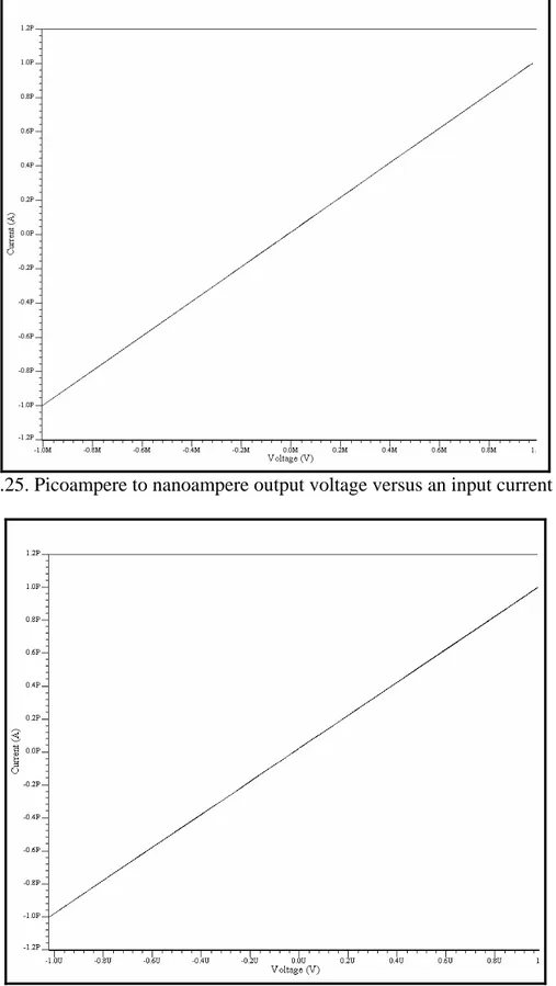
(9) Figure list Figure 1.1. Multiplexed Potentiostat Systems available in the market……………………..2 Figure 1.2. Diffusion field in macroelectrodes (left) and microelectrodes (right)………….3 Figure 1.3. Diagram of a single DNA spot inside a microfluidic channel with the PPy walls down for hybridization (left) and up for detection (right)…………………………………...4 Figure 2.1. Two-electrode cell (left) and three-electrode cell (right)……………………….7 Figure 2.2. Schematic representation of the equipment necessary to perform controlled – potential techniques ……………………………………………………...………………….8 Figure 2.3. Cyclic voltammograms for reversal at different E λ values…………………...11 Figure 3.1. Small signal electrode – electrolyte circuit model ignoring diffusion mechanisms………………………………………………………………………………...17 Figure 3.2. Small signal electrode – electrolyte circuit model including the diffusion (Warburg) impedance (Series) …………………………………………………………….18 Figure 3.3. Small signal electrode – electrolyte circuit model including the diffusion (Warburg) impedance (Parallel) …………………………………………………………...19 Figure 3.4. Behavior for the electronic model in figure 3.3……………………………….20 Figure 3.5. Circuit model of a metal microelectrode measurement system……………….21 Figure 3.6. Simplified circuit model of a metal microelectrode measurement system……21 Figure 3.7. Simplified circuit model for a glass microelectrode…………………………..21 Figure 3.8. Schematic of the electrochemical cell………………………………………...22 Figure 3.9. Electrochemical cell circuit model……………………………………………22 Figure 3.10 Impedance characteristics of electropointed tungsten microelectrodes………23 Figure 3.11. Model of the electrochemical cell to be used in the simulation of the potentiostat…………………………………………………………………………………23 Figure 4.1. Block diagram of the fully differential amperometric potentiostat measurement system concept for a single working measurement cell……………………………………26 Figure 4.2. Diagram of an individual potentiostat system………………………………..27 Figure 4.3. Circuit diagram of the frequency scheme……………………………………..28 Figure 4.4. Meassured output generated for a specific (a) current input voltage output across the (b) charging capacitor comparator output………………………………………29 Figure 4.5. Circuit to perform the PWM scheme………………………………………….30 Figure 4.6. PWM scheme signals………………………………………………………….30 Figure 4.7. Current input instrumentation amplifier………………………………………31 Figure 4.8. Output waveform for the high sensitivity IV scheme…………………………32 Figure 4.9. Circuit to perform the High sensitivity IV with capacitor scheme……………33 Figure 4.10. Response from currents of 10 pA and 1 nA with the S/H voltage…………...33 Figure 4.11. Circuit for controlling the potential at point eA regardless of changes in R1 and R2…………………………………………………………………………………………...35 Figure 4.12. Schematic of the control stage of the potentiostat………………………...…36 Figure 4.13. Symbol of the control stage of the potentiostat………………………...........36 Figure 4.14. Configuration used to hold the WE virtually connected to ground……………………...................................................................................................37. vi.

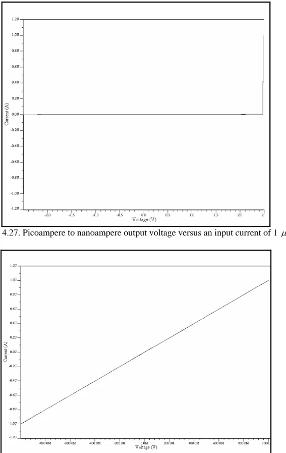
(10) Figure 4.15. Instrumentation amplifier…………………………………………………....38 Figure 4.16. Instrumentation amplifier for the 1 pA – 1 nA stage……………………..….39 Figure 4.17. Window comparator…………………………………………………………40 Figure 4.18. Offset adjustment circuit…………………………………………………..…40 Figure 4.19. Schematic of the sensitivity stage of the potentiostat………………………..41 Figure 4.20. Symbol of the sensitivity stage of the potentiostat…………………………..41 Figure 4.21. Schematic of the whole system………………………………………………42 Figure 4.22. Simulation results for a current of 1 pA with a Vscan of ± 1.5V……………..43 Figure 4.23. Simulation results for a current of 1500nA with a Vscan of ± 1.5V………….44 Figure 4.24. Offset voltages with Rs values of 1000, 10, 50, 70, 99, 235, 561, 1567 and 10000 Ω …………………………………………………….……………………………..45 Figure 4.25. Picoampere to nanoampere output voltage versus an input current of 1 pA…………………………………………………………………………………………..46 Figure 4.26. Nanoampere to microampere output voltage versus an input current of 1 pA…………………………………………………………………………………………..46 Figure 4.27. Picoampere to nanoampere output voltage versus an input current of 1 µ A…………………………………………………………………………………………47 Figure 4.28. Nanoampere to microampere output voltage versus an input current of 1 µ A…………………………………………………………………………………………47 Figure 5.1. a) NMOS transistor symbols [48] b) PMOS transistor symbols……………...50 Figure 5.2. Inverter schematic……………………………………………………………..50 Figure 5.3. MUX schematic……………………………………………………………….51 Figure 5.4. MUX symbol…………………………………………………….…………....52 Figure 5.5. Three signals MUX schematic……………………………………………….52 Figure 5.6. Three signals MUX symbol…………………………………………………..53 Figure 5.7. Block diagram of the multiplexed potentiostat system………………………..53 Figure 5.8. Potentiostat control stage coupled with two WEs at the electrochemical cell...54 Figure 5.9. Two potentiostat sensitivity stages coupled with two WEs…………………...55 Figure 5.10. Filters coupled with the special purpose MUX……………………………...55 Figure 5.11. Individual system response from sensing current 1 (15 pA)………………...56 Figure 5.12. Individual system response from sensing current 2 (10 pA)………………...57 Figure 5.13. Multiplexed signals…………………………………………………………..57 Figure 5.14. Multiplexed window signals…………………………………………………58 Figure 6.1. Electrodes labeling…………………………………………………………….60 Figure 6.2. Sensitivity stage for testing purposes………………………………………….62 Figure 6.3. Cyclic Voltammetry of experiment #01…………………………………........63 Figure 6.4. Cyclic Voltammetry of experiment #03……………………………………....64 Figure 6.5. Cyclic Voltammetry of experiment #05……………………………………....65 Figure 6.6. Cyclic voltammetry simulated on a recessed microelectrode array with an electrode radius of 10 µ m, distance between the electrodes in the array of 100 µ m and a recession depth of 10 µ m………………………………………………………………….66 Figure 6.7. Cyclic voltammetry simulated on a recessed microelectrode array with an electrode radius of 10 µ m, distance between the electrodes in the array of 100 µ m and a recession depth of 33 µ m………………………………………………………………….66. vii.

(11) Figure 6.8. Cyclic voltammetry simulated on a recessed microelectrode array with an electrode radius of 10 µ m, distance between the electrodes in the array of 100 µ m and a recession depth of 100 µ m………………………………………………………………...67 Figure 7.1. Sketch of the further work system………………………………………….....69 Figure B.1. Simulation results for a current of 10 pA with a Vscan of ± 1.5V…………….71 Figure B.2. Simulation results for a current of 100 pA with a Vscan of ± 1.5V…………...72 Figure B.3. Simulation results for a current of 500 pA with a Vscan of ± 1.5V…………...72 Figure B.4. Simulation results for a current of 1 nA with a Vscan of ± 1.5V………….......73 Figure B.5. Simulation results for a current of 10 nA with a Vscan of ± 1.5V…………….73 Figure B.6. Simulation results for a current of 100 nA with a Vscan of ± 1.5V…………...74 Figure B.7. Simulation results for a current of 500 nA with a Vscan of ± 1.5V…………...74 Figure B.8. Simulation results for a current of 750 nA with a Vscan of ± 1.5V…………...75 Figure B.9. Simulation results for a current of 1000 nA with a Vscan of ± 1.5V……….…75 Figure B.10. Simulation results for a current of 1pA with a Vscan of ± 2 V………………76 Figure B.11. Simulation results for a current of 1nA with a Vscan of ± 2 V………………76 Figure B.12. Simulation results for a current of 1000nA with a Vscan of ± 2 V……….….77 Figure B.13. Simulation results for a current of 2000nA with a Vscan of ± 2 V……….….77 Figure C.1. Individual system response from sensing current 1 (1.5 pA) ………………..79 Figure C.2. Individual system response from sensing current 2 (1 pA) ………………….80 Figure C.3. Multiplexed signals……………………………….…………………………..80 Figure C.4. Multiplexed window signals…………………………….……………………81 Figure C.5. Individual system response from sensing current 1 (15 nA) ………………...82 Figure C.6. Individual system response from sensing current 2 (25 nA) ………………...82 Figure C.7. Multiplexed signals………………………….………………………………..83 Figure C.8. Multiplexed window signals………………………………………………….83 Figure C.9. Individual system response from sensing current 1 (1 nA) ………………….84 Figure C.10. Individual system response from sensing current 2 (1.5 nA) ………………84 Figure C.11. Multiplexed signals………………………….………………………………85 Figure C.12. Multiplexed window signals………………………………………………...85 Figure C.13. Individual system response from sensing current 1 (500 pA) ……………...86 Figure C.14. Individual system response from sensing current 2 (1.5 nA) ………………86 Figure C.15. Multiplexed signals…….……………………….…………………………..87 Figure C.16. Multiplexed window signals…….…………………………………………..87 Figure C.17. Individual system response from sensing current 1 (500 pA) ……………...88 Figure C.18. Individual system response from sensing current 2 (500 nA) ……………...88 Figure C.19. Multiplexed signals……….…………………….…………………………...89 Figure C.20. Multiplexed window signals……….………………………………………..89 Figure C.21. Individual system response from sensing current 1 (150 pA) ……………...90 Figure C.22. Individual system response from sensing current 2 (100 pA) ……………...90 Figure C.23. Multiplexed signals……….……………………….………………………...91 Figure C.24. Multiplexed window signals……….………………………………………..91 Figure D.1. 5x amplification of sample 1a-d……………………………………………...92 Figure D.2. 10x amplification of sample 2a-d………………………………………….…92 Figure D.3. 20x amplification of sample 2a-d…………………………………………....93 Figure D.4. 20x amplification of sample 2a-d……………………………………………93. viii.

(12) Figure D.5. 20x amplification of sample 2a-d……………………………………………93 Figure D.6. 50x amplification of sample 2a-d…………………………………………….94 Figure D.7. 50x amplification of sample 2a.-d……………………………………………94 Figure D.8. 50x amplification of sample 2a.-d……………………………………………94 Figure D.9. 50x amplification of sample 2a.-d……………………………………………95 Figure D.10. 10x amplification of sample 3a-d…………………………………………...95 Figure D.11. 10x amplification of sample 6…………………………………………........95 Figure E.1. Cyclic Voltammetry of experiment #02……………………………………...96 Figure E.2. Cyclic Voltammetry of experiment #04…………………….………………..97. ix.

(13) Chapter 1 Introduction 1.1 Overview Knowing how the human brain works has been one of the biggest mysteries of mankind. By understanding the way cells interact with each other (in this case: neurons) it is possible to identify the real causes of diseases and to understand some cell disorders of which nowadays there is not much information available, for example Alzheimer [60]. Several years ago someone would have thought that the study of DNA chains was something too far away and impossible, yet this is a fact which has encouraged scientists to analyze DNA chains to detect diseases, among other applications. These examples demonstrate the need for technology that allows performing experiments regarding the study of biocells in an isolated way to set a framework for what up to now has been unknown to man. Furthermore, the pursuit of improving life quality has driven man to research, create and use technology as bioMEMs and microelectrodes in order to get faster response times, accurate and reliable data and other benefits which are reflected in medical applications for disease prevention and rehabilitation methods, to mention some. One of the technologies required to achieve the forementioned facts is the one that allows the study of individually addressable cells using microelectrodes array activation.. 1.2 Literature research Electrochemistry needs new tools and instrumentation to keep progressing as a science and many research groups, apart from companies, would benefit from the development of such instrumentation, which in this case refers to a truly multiplexed potentiostat. Recently, an electrochemical array microsystem with an integrated potentiostat has been proposed by Zhang et al. [19]. His 3x3 biosensor array based in CMOS covers the need of a protein based biomimetic sensor. This method shows a promising alternative for an assortment of electrochemical current based sensors [19]. Moreover, additional characteristics include the use of a load amplifier and an integrator based on switching capacitors.. 1.

(14) Other proposed solutions have been published in several papers; nevertheless, none of those meet the modularity feature which allows the flexibility to increase the array size as needed [21]. The table 1.1 summarizes the relevant publications previously made with potentiostats. Table 1.1. Comparison of previous publications with potentiostats. Paper Electrodes Multiplexed # WE Range Methodology Rezaul Hasan [29] Ferrero [27]. WE, RE WE, RE, AE. No No. n/a n/a. Zhang [19]. WE, RE, AE. Yes. 9. Yes. 128. 1 pA – 100 nA. No No. n/a n/a. 1 pA – 200 nA 0.1 – 3.5 µ A. WE, RE, AE. No. n/a. 0.1 nA – 0.5. n/a. Yes. 8 channel. pA to. Frey [30] Narula [32] Turner [25] Kakerow [24] Bandyopadhyay [37]. Generator E and Collector E, RE, AE WE, RE WE, RE. n/a nA - µ A 10 pA – 10. µA. (PGA). µA. µA. Current – Frequency Current – Voltage Current – Voltage using Capacitor Current – Number of pulses Current – Frequency n/a Current – Voltage using Capacitor n/a. Moreover, several multiplexed potentiostats are readily available from industrial manufacturers such as Gamry Instruments (Warminster, PA) and Princeton Applied Research (Oak Rigde, TN) [61, 62, 63]. Such devices are computer controlled, have a limited channel number and are big in size making them inadequate for bioMEMs medical applications [61, 62, 63]. Examples of these systems are MultEchem 8 Electrochemistry System that allows using 8 independent potentiostats installed all at the same time on industrial computers. Other examples are the VMP3 potentiostat from Princeton Applied Research and the Model 1000 Series Multi-Potentiostat from IJ Cambria Scientific/CH Instruments, which are computer controlled devices [61, 62, 63]. Despite the excellent performance of market instruments; characteristics as size, channel limitation and a PC requirement to control them makes them inadequate for bioMEMs applications due to the lack in flexibility and the cost. The figure 1.1 shows some multiplexed potentiostat systems available in the market.. Figure 1.1. Multiplexed Potentiostat Systems available in the market [61, 62, 63]. Just like these, several systems that allow addressing more than one working electrode are now available in the market. These systems are designed for highly specified applications. Nanogen Inc. (San Diego, CA) offers an electronic microarray for DNA 2.

(15) detection which is capable of activating 400 hybridization spots. Unfortunately, it is not possible to perform electrochemical measurements using this platform due to the fact that the DNA hybridization report takes place by fluorescent TAGS and not by electrochemical effects. Other research groups are working in a VLSI potentiostat of 16 channels for electroactive neurotransmitter detection [1, 2].. 1.3 Problem definition Despite microelectrodes have been used since 1980 and many technical references discuss their unique properties, the particular study of an individually addressable microelectrodes array behavior has not been totally developed due to the lack of appropriate testing platforms [3, 4]. The goal of this project is to develop a multiplexed potentiostat technology that will allow performing individual addressing of cells using microelectrode array activation. Such a device must be able to sense currents with high sensitivity in a microelectrodes array as to keep the modularity approach in order to further integrate additional microelectrodes to the system.. 1.4 Problem justification In the field of electrochemical measurements, microelectrodes that are smaller than the scale of the diffusion layer developed in readily executable experiments make it possible to take advantage of boundary effects (figure 1.2). These effects increase the mass transport of electroactive species on the surface of the working electrodes, thus increasing the performance of the device. The proposed platform will take advantage of this favorable miniaturization effect.. Figure 1.2. Diffusion field in macroelectrodes (left) and microelectrodes (right) [Image courtesy of Genis Turon Teixidor, UC Irvine] Another major advantage comes from individually addressing the arrayed electrodes. Being able to carry out potentiostatic experiments in microelectrodes that are very closely spaced will open up the possibility of measuring spatiotemporal concentration variations of electroactive species present in a solution.. 3.

(16) If this array of microelectrodes is installed in a microfluidic chamber, then it is possible to test models of mass transport in flows with low Reynolds number. There are also examples of biotechnology related applications that will take advantage of this multiplexed potentiostat. Very recently, in research collaboration between Prof. Ashutosh Sharma at the Indian Institute of Technology, Kanpur, and Prof. Marc Madou at the University of California, Irvine, single cell placement of an immortalized motor neuron cell line (NSC34) on top of a carbon electrode has been accomplished. Since this type of cells generate action potentials and show complex patterns of electrical activity, a method for individual stimulation is necessary to further understand their behavior as a network. A multiplexed potentiostat coupled with a recording system would serve this purpose. Other cell lines are also being considered. For instance, some researchers have suggested that is possible to influence the differentiation of stem cells by using electric and magnetic fields [5]. Once single cell placement will be achieved (like in the case of NSC-34 cells), the multiplexed potentiostat will make this study a reality. Another possible application example would be in drug delivery systems. The use of polypyrrole (PPy) bilayer micro actuators as an artificial muscle has been well studied, and this technology has proven to have many more far reaching applications. PPy is often used as an artificial muscle because it has the ability to shrink and expand based on the movement of ions in and out of the material [6]. Using a potentiostat, a voltage can be applied across the PPy and its solution. Ions will move in and out of the PPy based on the polarity and amplitude of that potential. When attached to a non expanding substrate, such as a thin gold layer, the shrinking and expanding of the PPy can cause the entire structure to bend and flex [6]. Using this concept, microfabricated flaps (figure 1.3) made of a PPy/gold bilayer can be produced. Prof. Marc Madou’s BioMEMS research group at UC Irvine has used this technology to produce drug-delivery capsules, in which PPy flaps are used as lids on microvials containing drugs [7]. A potentiostat is used to actuate the lids, thus releasing drugs from the vial. The next step in this project will be to array the device so that it can either a) contain many different drugs than need to be released at various times and/or locations or b) contain many small doses of the same drug so that it may provide a continuous dose response over a given period of time. Currently, it is only possible to operate a single lid and vial.. Figure 1.3. Diagram of a single DNA spot inside a microfluidic channel with the PPy walls down for hybridization (left) and up for detection (right). [Image courtesy of Jonathan Siegrist, UC Irvine]. 4.

(17) The field of DNA detection will also benefit from the development of a multiplexed potentiostat. So far, detection in DNA arrays has been performed either by optical detection equipment (like in the forementioned case of Nanogen Inc) or using enzyme based DNA arrays. Optical DNA arrays present major problems that prevent this procedure to be used in hospitals (i.e. high cost of optical detection equipment, difficulties in miniaturization and complex sample preparation [23]). Enzyme based DNA arrays present problems of crosstalk between spots, however they are a low cost solution due to the cheap detection strategies and they are relatively easy to miniaturize. A multiplexed potentiostat would enhance the efficiency of DNA microarray sensing reaching levels of a wider application of this method in hospital environments and general purpose laboratories.. 1.5 Scope The design of a multiplexed potentiostat will be treated in this thesis. Previous to the design of the multiplexed potentiostat, the design of a single potentiostat will be discussed. The design of such device is based in basic electronic instrumentation configurations, i.e. voltage follower, instrumentation amplifier, among others. The minimum resolution required is of the order of 1 pA. Subsequent to the design and simulations, it is intended to demonstrate the concept by means of experiments which implies the implementation of the design in a PCB and its integration with an electrochemical cell.. 1.6 Thesis content This thesis illustrates the theoretic framework and the development of a solution for the problem previously defined. The material is divided in seven chapters, references and the appendices. The first chapter gives an introduction to the problem and explains research previously made in the field as the advantages and disadvantages of the multiplexed potentiostat. The second chapter shows information concerning electrochemical instrumentation. Furthermore, the chapter describes the cyclic voltammetry technique and the need of specific instrumentation to perform such technique. Chapter three shows the electronic models for macro and microelectrodes as their equations and their integration to an electrochemical cell.. 5.

(18) Chapter four explains the potentiostat concept and the ways of solving the problem of concern. This chapter also treats the design of an individual potentiostat and the analysis of the results. Chapter five explains how to design the multiplexed potentiostat integrating the previous individual potentiostat desgined and shows the results of the whole system. Chapter six discusses the potentiostat testing. It explains the setup used for the experiment as the way the prototype was developed and its integration with an electrochemical cell in order to study the performance of the device. Chapter seven concludes this work by summarizing the achievements made and discussing some further work to enhance the potentiostat systems. The appendices provide some supplementary materials as follows: A. B. C. D. E. F.. Fick’s laws of diffusion Additional simulation results of the individual potentiostat Additional simulation results of the multiplexed potentiostat Electrode samples Testing results of the electrochemical cell LMP7721 amplifier data sheet. Finally, the bibliography presents 45 references coming from journals, reports or conferences, 14 specialized books or thesis and 11 sites from the WWW.. 6.

(19) Chapter 2 Electrochemistry Electrochemistry is the scientific branch that deals with the interaction of electrical and chemical effects. In electrochemical systems the focus is on the processes and factors that affect the transport of charge between chemical phases, for instance, between an electric conductor (an electrode) and an ionic conductor (an electrolyte). In order to study these phenomena, a very precise and accurate instrumentation is needed.. 2.1 Electrochemical instrumentation Electrochemical instrumentation generally consists of a potentiostat, for enforcing a controlled potential Eappl at an electrode (or a galvanostat, if the desire is to control the current i passing at this electrode), along with a function generator, to create the desired perturbation, and a recording and display system for measuring and representing i and Eappl with respect to a coordinate axis. Even though a great deal of innovation has been carried out throughout the last decades in the field of electrochemical instrumentation, mostly caused by the introduction of computer controlled systems, the basic testing electronic potentiostat circuit remains unchanged. In almost all configurations, there is a working electrode (the system of interest) coupled with an electrode of known potential called the reference electrode. In experiments involving large scale cells or non-aqueous solution with low conductivities, the current is passed between a working electrode and a counter (or auxiliary) electrode (figure 2.1). One of the most useful techniques that require the use of such instrumentation is cyclic voltammetry. Power supply. Power supply. i. i Reference electrode. Working electrode. Auxiliary electrode. Working electrode. Eappl. Eappl vs. ref. V. V. Reference electrode. Figure 2.1. Two-electrode cell (left) and three-electrode cell (right) [Image courtesy of Genis Turon Teixidor, UC Irvine] 7.

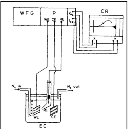
(20) Figure 2.2. Schematic representation of the equipment necessary to perform controlled – potential techniques. (WFG - Wave Form Generator. P - Potentiostat. CR - Chart Recorder. EC - Electrochemical cell. WE - Working Electrode. CE - Counter Electrode. RE Reference Electrode) [57]. As it can be inferred in figure 2.2, an electrochemical cell is required for the use of the potentiostat. The electrochemical cell consists of a vessel that can be sealed to prevent air entering into the solution, inlet and outlet ports to allow saturating the solution with an inert gas (N2 nitrogen or Ar Argon). Usually it is necessary to remove O2 (oxygen) to prevent currents due to the reduction of it interfering with the response of the system to be studied [57]. The standard cell configuration in this case consists of three electrodes immersed in the electrolyte: • • •. The working electrode (WE) The counter (CE) or auxiliary (AE) electrode The reference electrode (RE). The potential at the WE is monitored and controlled with respect to the RE via the potentiostat circuit. A desired waveform is imposed on the potential at the WE in order to measure the current flowing between the WE and the AE and a plot of I/V is obtained.. 8.

(21) 2.2 Measurement techniques There are two groups of techniques to measure variables in an electrochemical cell according to the controlled characteristic: current controlled and potential controlled. The techniques used to implement the potentiostat circuit require controlling the potential. In those techniques, the potential may be held constant or may be varied with time in a predetermined manner as the current is measured as a function of time or potential. These techniques contain one of the most powerful experimental set ups available in electrochemistry [46]. To apply those methods, the electrode area (A) must be small enough and the solution volume (V) large enough that the passage of current does not alter the bulk concentration of the electroactive species. Some of those techniques are linear potential sweep chronoamperometry, chronocoulometry, double potential step chronoamperometry, cyclic voltammetry and others. Nevertheless the proven usefulness in obtaining information about fairly complicated electrode reactions, cyclic voltammetry will be the technique of interest in this work. By means of this method, the formal redox potential of redox proteins (enzymes), an increase in the oxidation/reduction peak currents of DNA hybridization, and in general, electron transfer rate constants of redox couple reactions can be determined [41].. 2.2.1 Cyclic voltammetry Cyclic voltammetry (CV) was first reported in 1938 and described theoretically in 1948 by Randles and Sevcik. In cyclic voltammetry, a linear scanning potential is imposed for a stationary working electrode in the system. The potential is ramped between two chosen limits at a steady rate υ , then the potential is swept back and forth between the chosen limits one or more times. The current is monitored during the potential sweep [57]. Cyclic voltammetry is a reversal technique which has proven to be very useful in obtaining information about fairly complicated electrode reactions such as the presence of electro active species in the solution or on the electrode surface, the thermodynamics of redox processes, the kinetics of heterogeneous electron transfer reactions, and coupled chemical reactions or adsorption processes [40]. The reversal experiment in linear scan voltammetry is carried out by switching the direction of the scan at a certain time, t= λ , or at a switching potential, Eλ . Thus the. 9.

(22) potential is given at any time by equation 2.1 where ν is the scan rate, λ is the switching time, t is the time and Ei is the potential at which the experiment begins.. ⎧E - ν t E=⎨ i ⎩E i - 2νλ + νt. (0 < t ≤ λ ) (t > λ ). (2.1). The electron transfer of the redox reaction occurs at the WE, therefore the potential applied to the WE is scanned in a linear fashion between two potential values. The reaction occurs within the potential range defined. The potential at which the reduction or oxidation takes place provides qualitative information about the analyte of interest. The more negative this potential is, the better the reducing agent will be; on the other hand, the more positive the potential is the better the oxidizing agent will be. If the electronic transfer at the surface is fast and the current is limited by the diffusion of species to the electrode surface, the current peak will be proportional to the square root of the scan rate as in equation 2.2. i p = (2.69 x10 5 )n 3 / 2 ADO. 1/ 2. CO ν 1 / 2 *. (2.2). In equation 2.2 is assumed an electrode area A in cm2, an oxidizing species diffusion coefficient DO in cm2/s, an initial concentration of the oxidizing species CO* in mol/cm3, a scan rate ν in V/s, and the stoichiometric number of electrons, n, involved in an electrode reaction to obtain a peak current in amperes. In the case of a CV expected from an electroactive adsorbed species it is assumed that [57]: 1) At time t= 0 the electrode surface has the maximum coverage of the oxidized form, O. 2) The electrochemical reaction can be represented by O + ne- ÍÎ R and is kinetically fast enough to maintain Nernstian behavior at each point in the CV scan such that the concentrations of O and R near the electrode obey the Nernst equation, where O is the oxidizing species, R is the reducing species and ne- is the number of negative carriers. 3) The oxidized and reduced species are both strongly adsorbed and have the same enthalpy of adsorption. 4) There is no O or R in the solution. In figure 2.3, cyclic voltammograms for reversal at different E λ values are presented in an i – E format. Cathodic (positive) and anodic (negative) currents are represented where cathodic current is the current generated as a result of the reduction in the electrode, that is to say, the flow of electrons from the electrode to a species in solution. Moreover, the. 10.

(23) anodic current is the result of the oxidation process produced by the reversal experiment, that is, the flow of electrons from a species in solution to the electrode.. Figure 2.3. Cyclic voltammograms for reversal at different E λ values [46] The shape of the curve on reversal depends on the switching potential, E λ , or how far beyond the cathodic peak the scan can proceed before reversal. On these i – E curves, two measured parameters of interest are the ratio of peak currents, ipa/ipc (ipa anodic peak current, ipc cathodic peak current), and the separation of peak potentials, Epa – Epc (Epa anodic peak potential, Epc cathodic peak potential). For a wave with stable product ipa/ipc will be one regardless of scan rate, E λ (for E λ >35/n mV past Epc) and diffusion coefficients. Deviation of the ratio ipa/ipc from unity is indicative of homogeneous kinetic or other complications in the electrode process. If the cathodic sweep is stopped and the current is allowed to decay to zero, the resulting anodic i – E curve is identical in shape to the cathodic one, but is plotted in the opposite direction on both the i and E axes. This occurs because it allows the cathodic current to decay to zero and results in the diffusion layer being depleted of O and populated. 11.

(24) with R at a concentration near CO* (bulk concentration), so that the anodic scan is virtually the same as that which would result from an initial anodic scan in a solution containing only R [46]. The difference between Epa and Epc ( ∆E p ) is a useful diagnostic test of a reaction. This difference, ∆E p , is always close to 59/n mV at 25 °C. One of the problems of CV is its imprecision while measuring peak currents since the correction for charging current is typically uncertain. For the reversal peak, the imprecision is increased further because one cannot readily define the folded faradaic response during the forward process to use as a reference for the measurement [46]. Summarizing the cyclic voltammetry process: • • • • • • •. A voltage is varied in a solution Current (faradic) is measured respect to ∆ V (cyclic voltammogram) Is used to study redox properties of chemicals. Electroactive species is in the form of a solution. A potential is controlled between the WE and the RE. Current flows from the AE to the WE. Current increases as potential approaches to the reduction potential of the analyte.. 2.2.2 Theoretical treatment of cyclic voltammetry Nernstian (Reversible) Systems For this theoretical treatment, the reaction O + ne ↔ R is considered, assuming semiinfinite linear diffusion and a solution initially containing only species O (O Oxidation, R Reduction, ne stoichiometric number of electrons). Semi – infinite linear diffusion and a solution initially containing only species O is expressed by Fick’s laws [46] in equations 2.3 and 2.6 (for a better understanding of Fick’s laws refer to appendix A). Boundary conditions are expressed in equations 2.4, 2.5, 2.7 and 2.8. dC O ( x, t ) d 2 C O ( x, t ) = DO dt dx 2. (2.3). CO ( x,0) = CO. (2.4). *. lim x→∞ CO ( x, t ) = CO. 12. *. (2.5).

(25) dC R ( x, t ) d 2 C R ( x, t ) = DR dt dx 2. (2.6). C R ( x,0) = 0. (2.7). lim x→∞ C R ( x, t ) = 0. (2.8). Boundary conditions say that the initial concentration of O at a distance x (CO(x,0)) from the electrode’s surface is the bulk concentration of O (CO*) and implies that the concentration of the species R is initially absent but will be produced according to the flux balance equation expressed in equation 2.9. DO. dC O ( x, t ) dx. + DR x =0. dC R ( x, t ) dx. =0. (2.9). x =0. Each CV experiment begins at a potential Ei where no electrode reaction occurs, that is, at which no current flows; and at t = 0. The potential is swept linearly at υ (V/s) so that the potential at any time is expressed by equation 2.10; extracted from a previously posed equation 2.1. E (t) = Ei - 2 υ λ + υ t. (2.10). If it is assumed that the charge transfer kinetics are very rapid so that species O and R immediately adjust to the ratio dictated by the Nernst equation, such behavior is expressed by equation 2.11 where E 0´ is the electrode formal potential, R is the Rankin gas constant equal to 8.31447 J mol-1 K-1, T is the absolute temperature equal to 273 °K, n is the stoichiometric number of electrons involved in an electrode reaction, F is the faraday constant equal to 9.64853x104 C, C O (0, t ) is the concentration of the oxidizing specie at the electrode surface at a time t, C R (0, t ) is the concentration of the reducing specie at the electrode surface at a time t, DO is the diffusion coefficient of the oxidizing specie and DR is the diffusion coefficient of the reducing specie.. E = E 0' +. RT CO (0, t ) ln nF C R (0, t ). (2.11). This Nernst equation can be developed to express the relation between the species concentration as expressed in equation 2.12.. f (t ) =. (. ). CO (0, t ) ⎤ ⎡ nF E − E 0' ⎥ = exp⎢ C R (0, t ) ⎦ ⎣ RT. 13. (2.12).

(26) Therefore, equation 2.10 is substituted in equation 2.12 originating the development of 2.13, 2.14 and 2.15.. f (t ) =. f (t ) =. (. ). C O (0, t ) ⎤ ⎡ nF Ei − 2νλ + νt − E 0 ' ⎥ = exp ⎢ C R (0, t ) ⎦ ⎣ RT. (. (2.13). ). CO (0, t ) nF ⎤ ⎡ nF Ei − E 0 ' + = exp⎢ (−2νλ + νt )⎥ RT C R (0, t ) ⎦ ⎣ RT. (. CO (0, t ) ⎡ nF Ei − E 0' = exp ⎢ C R (0, t ) ⎣ RT. nF ⎤ )⎤⎥ exp⎡⎢ RT ν (−2λ + t )⎥ ⎦. ⎦. ⎣. (2.14). (2.15). The first exponential in equation 2.15 is defined as the constant θ as follows:. (. ). ⎡ nF ⎤ Ei − E 0 ' ⎥ ⎣ RT ⎦. θ = exp ⎢. (2.16). In the second exponential in equation 2.15, the constant terms are defined as σ and LaPlace (S (t)) as follows: S(t) = eσt − 2σλ for (t > λ ) and σ =. nF ν RT. (2.17). In consequence, according to Bard [46], the boundary condition, which is the relation between O and R concentrations in the boundary (electrode surface), can be written as:. CO (0, t ) = θe σt − 2σλ = θS (t ) C R (0, t ). (2.18). and from using the equation A.2 and relating it to the forementioned equations, it is possible to determine the concentration of an O species from the current flowing in an electrochemical experiment, or predict the current flow expected on an electrochemical experiment according to the initial concentration of a species. For further and deeper theoretical treatment about cyclic voltammetry refer to the Cottrell equation and diffusion in UMEs (ultramicroelectrodes) [46].. 2.3 Glance to the future With the use of a multiplexed potentiostat and the cyclic voltammetry technique it could be possible to know the concentration of species in an electrochemical cell according to the current measured on its working electrode and relate those concentrations to the. 14.

(27) presence of a disease. Therefore, once the procedure is finished, a preventive medicine is used to avoid such a disease. With microinstrumentation that allows performing this kind of measurements it would be possible to reduce spaces in hospitals and to transport such instrumentation to remote areas. Moreover, it would be possible to have better and faster diagnostic tools, on – line rapid analytic instrumentation, cheaper development and medical treatment, prevention of illness. The tendency is to miniaturize equipment, to reduce response times and to decrease costs when applying cyclic voltammetry technique to daily life. For example, replacing the fluorescence imaging, immunochemical and liquid chromatography methods to detect and measure neurotransmitter activity for an electrochemical analysis [23]. Another further use is to use biosensor chips such as DNA and protein arrays to avoid expensive optical set – ups as CCD cameras, lenses, etc. [20] and to perform detection in DNA arrays with a microchip instead of optical methods that require expensive and voluminous equipment [23].. 15.

(28) Chapter 3 Electrochemical cell modeling This chapter presents a description of the electrical model for electrodes in order to provide a good dynamic simulation of the potentiostat circuit. To understand the electric behavior of electrodes and chemical cells it is necessary to have an equivalent circuit model which represents the small signal behavior. A simplified RC circuit model will be used to represent the electrode. The ohmic resistance will be considered as well. Furthermore, the effect of charging and discharging the leaking capacitance will be modeled.. 3.1 Electrodes The electrode constitutes the fundamental interface between the ionic and electronic currents. An adequate set of electrodes provides a great insight into the solution of the potentiostat circuit. The electrodes in the electrochemical instruments are like the antennas in the reception of electromagnetic waves.. 3.1.1 Macroelectrodes: Randles equivalent circuit To understand the small signal electrical properties of electrodes, it is necessary to recall that a space charge region is formed at the interface in the electrochemical cell between a metal and an electrolyte. A change in the total potential difference resulting from the current flowing alters the charge distribution in a nonlinear manner. This phenomenon is represented by a leaking capacitance (Ch) whose value depends on the steady state current and allows the small signal displacement current and voltage to be related [58]. Furthermore, a resistance Rt represents the charge transfer incremental resistance. Rt and Ch are frequency independent and do not include the diffusion effects. The figure 3.1 shows the small signal electrode – electrolyte circuit model ignoring diffusion mechanisms where Ch is the double layer incremental capacitance and Rt is the charge transfer incremental resistance The capacitance Ch is given by equation 3.1.. 16.

(29) Ch =. dQ dV. (3.1). Figure 3.1. Small signal electrode – electrolyte circuit model ignoring diffusion mechanisms [58]. For an electrode in which the steady state current is such that nt << RT / αzF , the charge transfer incremental resistance is given by equation 3.2 where z is the transfer valence, α is the transfer coefficient, nt is the electrode overvoltage, R, T and F were defined on chapter 2, I0 is defined as the current flowing and J0 is the exchange current density. Rt =. dI RT 1 = dnt zF I 0. (3.2). For an electrode in which the steady state current is such that nt >> RT / αzF the charge transfer incremental resistance is given by equation 3.3. Rt =. RT 1 αzF I. (3.3). Therefore, the current density J0 and electrode overvoltage η t are related by equation 3.4. J ⎛ αznt F ⎞ ⎛ − (1 − α ) znt F ⎞ = exp⎜ ⎟ − exp⎜ ⎟ J0 RT ⎝ RT ⎠ ⎝ ⎠. (3.4). Furthermore, equation 3.4 applies if the charge transfer overvoltage mechanism is the dominant cause of the electrode overvoltage (which is the case for an electrode with a small exchange current density) [58].. 17.

(30) Thus far, as the figure 3.1 shows, the small signal model of an electrode consists of two parallel linear elements that are frequency independent but the model operating in steady state shows current nonlinearly dependency. The figures 3.2 and 3.3 show a small signal electrode – electrolyte circuit model that includes the diffusion (Warburg) impedance. This model includes two frequency dependent elements to represent the effects of diffusion.. Figure 3.2. Small signal electrode – electrolyte circuit model including the diffusion (Warburg) impedance (Series) [58]. . The figure 3.2 shows the series configuration where Ch and Rt were previously defined. Moreover, Rd and Cd are the Warburg series equivalent impedance elements representing the diffusion effects. For conditions close to equilibrium and for single ion species domination diffusion, the series elements are given by equations 3.5, 3.6 and 3.7 where D is the diffusion coefficient, ω is the frequency, and C0 is the ion concentration under equilibrium conditions. Rd =. RT z2F 2. z2F 2 RT 1 Rd C d =. Cd =. 1 1 2ω C 0 D. (3.5). 2. (3.6). ω. ω. C0 D. (3.7). Hence, the diffusion or Warburg impedance can be written as defined by equations 3.8 and 3.9.. 18.

(31) Z w = Rd +. 1 = Rd (1 − j ) jω C d. (3.8). ω. (3.9). ∴ Zw ∝ 1. The figure 3.3 shows a parallel configuration for the elements that represent the diffusion impedance, the Warburg elements are expressed by equations 3.10, 3.11 and 3.12. Rd =. RT z2F 2. z2F 2 RT 1 Rd C d =. Cd =. 2. 1. (3.10). ω C0 D 1 C0 D 2ω. ω. (3.11). (3.12). Figure 3.3. Small signal electrode – electrolyte circuit model including the diffusion (Warburg) impedance (Parallel) [58]. When using the Warburg impedance, it is reasonable to expect a low pass effect (arising from diffusion process) which means that the impedance’s magnitude will decrease toward zero as the frequency increases [58]. Figure 3.4 shows the theoretical behavior of the electronic model in figure 3.3. It shows over a log frequency scale how the impedance’s magnitude behaves. Values of the phase angle for various frequencies are indicated along the top horizontal axes. Furthermore, if a series resistor is added in any of those models, the bulk resistance of the electrolyte RB could be considered and this equivalent circuit is now the complete model.. 19.

(32) Figure 3.4. Behavior for the electronic model in figure 3.3 [58]. 3.1.2 Microelectrodes. There are different kinds of microelectrodes: metal microelectrode, carbon microelectrode, etc. The electrical properties of these microelectrodes differ considerably [58]. Figures 3.5 and 3.6 show a circuit model for a metal microelectrode measurement system to perform intracellular measurements.. 20.

(33) Figure 3.5. Circuit model of a metal microelectrode measurement system [58].. Figure 3.6. Simplified circuit model of a metal microelectrode measurement system [58].. The figures 3.5 and 3.6 illustrate the models when performing an intracellular measurement. There, Rs is the spreading resistance which arises from the electrolyte resistance in the vicinity of the metal tip, Rm is the bulk resistance of the metal, Cs shunts the signal to be measured and its value depends on the permittivity and thickness of the insulator as well as on the depth of immersion, Re and Ce are the metal electrolyte parallel components which are frequency dependent. Ecell is the cell potential and Zcell is the cell impedance. The figure 3.7 shows a simplified circuit model for a glass microelectrode where R is the bulk resistance of the electrolyte in the tip region and C is the capacitance across the glass wall between the filling and test solutions dependent on the depth to which the electrode is immersed. In this model, the spreading resistance of the solution surrounding the tip and the impedance of the inner reference electrode can be neglected in comparison to R. Ec is the cell potential, Ej represents the liquid junction potential and Et, the tip potential.. Figure 3.7. Simplified circuit model for a glass microelectrode [58]. 21.

(34) 3.2 Electrochemical cell. An electrochemical cell can be regarded as a network of impedances, therefore, the symmetry in the design and placement of the working and counter electrodes is important. The resistance between the working and auxiliar electrodes directly controls the power levels required from the potentiostat and the resistive heating in bulk electrolysis that might have to be dissipated by cooling. Therefore, having the electrodes close together is much better to allow an optimized performance of the electrolysis process [46].. Figure 3.8. Schematic of the electrochemical cell [27] The figure 3.8 shows the schematic of an electrochemical cell. The figure 3.9 shows the circuit model of this cell. According to [19], Rs and Ru are the resistances of the solution between the electrodes where Ru is the uncompensated resistance originated if the RE is placed anywhere but exactly at the working electrode surface, Rfw represents the faradaic resistance and Cd represents the double layer capacitance associated with the WE.. Figure 3.9. Electrochemical cell circuit model [19] The faradaic resistance depends on the electrochemical parameters of the electrolyte (analyte) and on the molar concentration of the generated electrochemical products [29]. According to [37], Rs is usually lower that 100 Ω , Icell < 10 µ A, and Rfw according to [58] has values in the range of M Ω for a microelectrode. 22.

(35) The figure 3.10 shows the impedance characteristics for an electropointed tungsten microelectrode along with an increase in frequency. In the figure, ∆ indicates unplated; χ , plated with bright Pt; o, plated with black Pt. The dimensions of the exposed conical tip before plating were 20 µ m of length and 6 µ m of diameter. The plating thicknesses were between 1 and 2 µ m and the bars at 10 Hz indicate the range of impedance values encountered with electrodes of the same nominal dimensions [58].. Figure 3.10 Impedance characteristics of electropointed tungsten microelectrodes [58]. 3.2.1 Electrochemical cell model for the potentiostat design. The circuit model of the electrochemical cell in figure 3.9 will be coupled with a current source as figure 3.11 shows in order to test the sensitivity of the system.. Figure 3.11. Model of the electrochemical cell to be used in the simulation of the potentiostat [19]. 23.

(36) It is important to remember that Rs and Ru are the resistances of the solution; in this case, Ru can be made negligibly small by careful placement of the reference electrode [46]. Rfw represents faradaic resistance and Cd, the double layer capacitance associated with the working electrode. According to [58] the values of Rfw and Cd will decrease with increasing frequency. For example, a 10 µm 2 area electrode may exhibit a 100 M Ω impedance at 1 kHz. The current source in the electrochemical cell of figure 3.11 has testing purposes of the sensitivity of the measurement circuit in the simulations, by generating a current equivalent to the faradaic current generated by the redox reaction.. 24.