Assessment of Land Cover Change Effect on the San Juan River Watershed Hydrology in Nuevo León México Edición Única

Texto completo

(1)INSTITUTO TECNOLÓGICO Y DE ESTUDIOS SUPERIORES DE MONTERREY. CAMPUS MONTERREY DIVISIÓN DE INGENIERÍA Y ARQUITECTURA PROGRAMA DE GRADUADOS EN INGENIERÍA. Assessment of land cover change effect on the San Juan River watershed hydrology in Nuevo Leon, Mexico.. TESIS PRESENTADA COMO REQUISITO PARCIAL PARA OBTENER EL GRADO ACADÉMICO DE:. MAESTRO EN CIENCIA ESPECIALIDAD EN SISTEMAS AMBIENTALES. POR: AXAYÁCATL MAQUEDA ESTRADA. MONTERREY, N.L.. MAYO 2008.

(2) INSTITUTO TECNOLÓGICO Y DE ESTUDIOS SUPERIORES DE MONTERREY CAMPUS MONTERREY DIVISIÓN DE INGENIERÍA Y ARQUITECTURA PROGRAMA DE GRADUADOS EN INGENIERÍA. Los miembros del comité de tesis recomendamos que la presente tesis del Ing. Axayácatl Maqueda Estrada sea aceptada como requisito parcial para obtener el grado académico de Maestro en Ciencias especialidad en:. SISTEMAS AMBIENTALES. Comité de Tesis:. __________________________ Dr. Diego Fabián Lozano García Asesor. _________________________ Dr. Jianhong Ren Sinodal. __________________________ Dr. Kim Jones Sinodal. Aprobado:. _________________________ Dr. Joaquín Acevedo Mascarúa Director de Investigación y Posgrado de la Escuela de Ingeniería Mayo, 2008.

(3) ABSTRACT. Assessment of land cover change effect on San Juan River watershed hydrology in Nuevo Leon Mexico (August 2007) Axayacatl Maqueda Estrada, B.A. ITESM Monterrey, Mexico Chairman of advisory committee: Dr. Jianhong Ren. The San Juan River is a part of the Rio Grande/Bravo watershed in the Mexican territory. For many years the San Juan River watershed has been altered by deforestation, which is related to agricultural and urban development. Deforestation can lead to changes in water availability in the watershed. A computer model (Soil and Water Assessment Tool) was used to relate physical characteristics such as soil type, rainfall and land cover type with the water balance of the watershed. The use of the computer was based on the lack of internal gauge stations data in the watershed. There is data from one station at the watershed outlet. However, the computer model allows to get results for specific areas of the watershed. Land cover data from year 1974, 1998 was available for the assessment. Also an estimated land cover map was created for year 2020 considering the growth of urban areas. Modeling results show a significant relation between land cover change and water flows behavior and how small changes in areas of the watershed can produce considerable changes in water flow, i.e. a increase of 19% of the size of urban areas caused an increase of 64% in the surface runoff in the Urban Areas region of the watershed. Model flow results from year 1974, 1998 and 2020 were compared to assess the effect of land cover change on the hydrological processes of the watershed.. iii.

(4) ABSTRACT IN SPANISH. Assessment of land cover change effect on San Juan River watershed hydrology in Nuevo Leon Mexico (August 2007) Axayacatl Maqueda Estrada, B.A. ITESM Monterrey, Mexico Chairman of advisory committee: Dr. Jianhong Ren. El Río San Juan es parte de la cuenca del río Bravo dentro del territorio de México. Por muchos años la cuenca del Río San Juan ha sido alterada por la deforestación. La deforestación puede producir cambios en la disponibilidad de agua en la cuenca. Un modelo por computadora (SWAT, Soil and Water Assessment Tool) fue utilizado para relacionar las características físicas de la cuenca como el tipo de suelo, la precipitación, y el tipo de cobertura vegetal con el balance de agua de la cuenca. El uso del modelo por computadora se basó en la falta de datos de estaciones hidrométricas en el interior de la cuenca. Sin embargo el modelo por computadora permite obtener resultados para áreas específicas de la cuenca. Datos de cobertura vegetal del suelo del año 1974, 1998 fueron utilizados en la modelación. También se creó una cobertura vegetal del suelo para el año 2020 considerando los pronósticos de crecimiento de las áreas urbanas. Los resultados de la modelación muestran una relación importante entre cambios de la cobertura vegetal y el comportamiento de las corrientes de agua. Resultados del modelo basados en condiciones del año1974, 1998 y el 2020 fueron comparados entre sí para evaluar el efecto del cambio de uso de suelo en los procesos hidrológicos de la cuenca.. iv.

(5) AGRADECIMIENTOS. A mis asesores y maestros, M.C. Ing. Kevin Luna Villarreal, Dr. Salvador García Rodríguez y Dr. Juan Pablo Solís gracias pos su tiempo y sus valiosas aportaciones para hacer de esta una tesis completa.. A mis maestros de la maestría gracias por enseñarme tod aquello que dice la teoría y mas por enseñarme todo lo que no dice.. A todos mis amigos, los que he conocido durante todo el recorrido y a mis amigos de la maestría gracias por abrirme los ojos a un nuevo mundo de conocimiento y aprendizaje.. iv.

(6) TABLE OF CONTENTS ABSTRACT . . . . . . . . . . . . . . . . . . . . . . . . . . . . . . . . . . . . . . . . . . . . . . . . . . . . . . . . . . . iii ABSTRACT IN SPANISH . . . . . . . . . . . . . . . . . . . . . . . . . . . . . . . . . . . . . . . . . . . . . . . . iv ACKNOWLEDGMENT . . . . . . . . . . . . . . . . . . . . . . . . . . . . . . . . . . . . . . . . . . . . . . . . . . v TABLE OF CONTENTS . . . . . . . . . . . . . . . . . . . . . . . . . . . . . . . . . . . . . . . . . . . . . . . . . vi LIST OF FIGURES . . . . . . . . . . . . . . . . . . . . . . . . . . . . . . . . . . . . . . . . . . . . . . . . . . . . viii LIST OF TABLES . . . . . . . . . . . . . . . . . . . . . . . . . . . . . . . . . . . . . . . . . . . . . . . . . . . . . . xi CHAPTER I. INTRODUCTION . . . . . . . . . . . . . . . . . . . . . . . . . . . . . . . . . . . . . . . . . . . . 1 CHAPTER II. LITERATURE REVIEW . . . . . . . . . . . . . . . . . . . . . . . . . . . . . . . . . . . . . 3 2.1 Water balance. . . . . . . . . . . . . . . . . . . . . . . . . . . . . . . . . . . . . . . . . . . . . . . . . . 3 2.2 Effects of land cover type change on watershed hydrology . . . . . . . . . . . . . . 5 2.3 Watershed models and modeling . . . . . . . . . . . . . . . . . . . . . . . . . . . . . . . . . . . 8 CHAPTER III. PROBLEM IDENTIFICATION . . . . . . . . . . . . . . . . . . . . . . . . . . . . . . 12 3.1 Problem definition . . . . . . . . . . . . . . . . . . . . . . . . . . . . . . . . . . . . . . . . . . . . . 12 3.2 Objectives . . . . . . . . . . . . . . . . . . . . . . . . . . . . . . . . . . . . . . . . . . . . . . . . . . . 14 CHAPTER IV. METHODOLOGY . . . . . . . . . . . . . . . . . . . . . . . . . . . . . . . . . . . . . . . . . 16 4.1 Description of study area . . . . . . . . . . . . . . . . . . . . . . . . . . . . . . . . . . . . . . . . 16 4.2 Modeling approach . . . . . . . . . . . . . . . . . . . . . . . . . . . . . . . . . . . . . . . . . . . . 30 4.2.1 AGWA tool and SWAT model . . . . . . . . . . . . . . . . . . . . . . . . . . . . 30 4.2.2 SCS Curve Number method . . . . . . . . . . . . . . . . . . . . . . . . . . . . . . 33 4.3 Mexico’s soil classification system and hydrological parameters . . . . . . . . . 35 4.4 Mexico’s land cover classification system and vegetation parameters . . . . . 44 4.4.1 Years 1974 and 1998 land cover data . . . . . . . . . . . . . . . . . . . . . . . 44 4.4.2 Year 2020 land cover data (estimated) . . . . . . . . . . . . . . . . . . . . . . 48 CHAPTER V. RESULTS AND DISCUSSION . . . . . . . . . . . . . . . . . . . . . . . . . . . . . . . 49 5.1 Rainfall variation trough study period . . . . . . . . . . . . . . . . . . . . . . . . . . . . . . 49 5.2 SWAT model runs . . . . . . . . . . . . . . . . . . . . . . . . . . . . . . . . . . . . . . . . . . . . . 53 5.3 SWAT treatment of rainfall data . . . . . . . . . . . . . . . . . . . . . . . . . . . . . . . . . . 54 5.4 SWAT model calibration for surface runoff . . . . . . . . . . . . . . . . . . . . . . . . . 55 5.5 Land cover changes trough study period . . . . . . . . . . . . . . . . . . . . . . . . . . . . 59. vi.

(7) 5.6 Modeling results . . . . . . . . . . . . . . . . . . . . . . . . . . . . . . . . . . . . . . . . . . . . . . . 66 5.6.1 Annual results . . . . . . . . . . . . . . . . . . . . . . . . . . . . . . . . . . . . . . . . . 66 5.6.2 Monthly results . . . . . . . . . . . . . . . . . . . . . . . . . . . . . . . . . . . . . . . . 71 5.6.3 Watershed hydrological response to a major rainfall event . . . . . . 77 5.7 Discussion . . . . . . . . . . . . . . . . . . . . . . . . . . . . . . . . . . . . . . . . . . . . . . . . . . . 83 CHAPTER VI. SUMMARY AND CONCLUSIONS . . . . . . . . . . . . . . . . . . . . . . . . . . 86 CHAPTER VII. FURTHER RESEARCH . . . . . . . . . . . . . . . . . . . . . . . . . . . . . . . . . . . . 89 REFERENCES . . . . . . . . . . . . . . . . . . . . . . . . . . . . . . . . . . . . . . . . . . . . . . . . . . . . . . . . 91 APPENDIX . . . . . . . . . . . . . . . . . . . . . . . . . . . . . . . . . . . . . . . . . . . . . . . . . . . . . . . . . . . 95 VITA . . . . . . . . . . . . . . . . . . . . . . . . . . . . . . . . . . . . . . . . . . . . . . . . . . . . . . . . . . . . . . . .102. vii.

(8) LIST OF FIGURES. Figure 4.1 States in Mexico and USA that are part of Bravo River watershed . . . . . . . . 17 Figure 4.2 Study area within San Juan River watershed . . . . . . . . . . . . . . . . . . . . . . . . . 19 Figure 4.3 Distribution of rainfall on San Juan River watershed . . . . . . . . . . . . . . . . . . 20 Figure 4.4 Weather types in study area according to Köppen classification, modified by Enriqueta Garcia . . . . . . . . . . . . . . . . . . . . . . . . . 21 Figure 4.5 Landsat image of San Juan River watershed and regions . . . . . . . . . . . . . . . 24 Figure 4.6 Land cover in Agriculture region, grasslands and tree farms . . . . . . . . . . . . . 25 Figure 4.7 Topography and land cover in Forest region, mountains and forests . . . . . . . 26 Figure 4.8 Typical land cover type on Huajuco Canyon . . . . . . . . . . . . . . . . . . . . . . . . . 27 Figure 4.9 Typical land cover and landscape for Huasteca Canyon . . . . . . . . . . . . . . . . 28 Figure 4.10 Land cover for Urban Area region: high density urbanization . . . . . . . . . . 29 Figure 4.11 Hydrological soil types in San Juan River Watershed . . . . . . . . . . . . . . . . 43 Figure 5.1 Rainfall data for all weather stations in the studied watershed in years a) 1974, b) 1975, c) 1998, and d) 1999 . . . . . . . . . . . . . . . . . . . . . . 51 Figure 5.2 Location of weather stations in study area . . . . . . . . . . . . . . . . . . . . . . . . . . . 52 Figure 5.3 River flow for year 1974 before model calibration . . . . . . . . . . . . . . . . . . . . 56 Figure 5.4 Model calibration results for year 1974 . . . . . . . . . . . . . . . . . . . . . . . . . . . . . 57 Figure 5.5 Model calibration results for a) year 1986, and b) year 1994 . . . . . . . . . . . . 58 Figure 5.6 Land cover type areas for year 1974 . . . . . . . . . . . . . . . . . . . . . . . . . . . . . . . 60 Figure 5.7 Land cover type areas for year 1998 . . . . . . . . . . . . . . . . . . . . . . . . . . . . . . . 61 Figure 5.8 Estimated land cover type areas for year 2020 . . . . . . . . . . . . . . . . . . . . . . . . 62 Figure 5.9 Areas of land cover modified from year 1998 to create land cover for year 2020 . . . . . . . . . . . . . . . . . . . . . . . . . . . . . . . . . . . . . . . . 63. viii.

(9) Figure 5.10: 1974 percent contribution of each land cover type to total area . . . . . . . . . 64 Figure 5.11 1998 percent contribution of each land cover type to total area . . . . . . . . . . 65 Figure 5.12 2020 percent contribution of each land cover type to total area . . . . . . . . . . 65 Figure 5.13 Simulated annual average flow data for the whole study area obtained from SWAT model (annual averages) . . . . . . . . . . . . . . . . . . . . . 66 Figure 5.14 Ratios of surface runoff to baseflow . . . . . . . . . . . . . . . . . . . . . . . . . . . . . . 68 Figure 5.15 Annual average percolation and percent change in years 1998 and 2020 compared with that in year 1974. . . . . . . . . . . . . . . . . . . . . . 69 Figure 5.16 Simulated annual average surface flow . . . . . . . . . . . . . . . . . . . . . . . . . . . . 70 Figure 5.17 Simulated annual average baseflow . . . . . . . . . . . . . . . . . . . . . . . . . . . . . . . 71 Figure 5.18 Monthly averages of surface runoff in the Forest region . . . . . . . . . . . . . . . 72 Figure 5.19 Monthly averages of baseflow in the Forest region. . . . . . . . . . . . . . . . . . . 72 Figure 5.20 Monthly averages of surface flow in the Huajuco Canyon region. . . . . . . . 73 Figure 5.21 Monthly averages of baseflow in the Huajuco Canyon region . . . . . . . . . . 74 Figure 5.22 Monthly averages of surface flow in the Huasteca Canyon region. . . . . . . . 75 Figure 5.23 Monthly averages of baseflow in the Huasteca Canyon region . . . . . . . . . . 75 Figure 5.24 Monthly averages of surface flow in the Urban Areas region . . . . . . . . . . . 76 Figure 5.25 Monthly averages of baseflow in the Urban Areas region . . . . . . . . . . . . . . 77 Figure 5.26 Daily rainfall for September 1988 . . . . . . . . . . . . . . . . . . . . . . . . . . . . . . . . 78 Figure 5.27 Simulated water flows for whole study area for September 1988 . . . . . . . . 80 Figure 5.28 Simulated surface flow for September 1988 by regions . . . . . . . . . . . . . . . 81 Figure 5.29 Simulated baseflow for September 1988 by regions . . . . . . . . . . . . . . . . . . 82 Figure 9.1.1 Comparison between simulated and actual rainfall for weather stations in year 1974 before SWAT model calibration . . . . . . . . . . . . . . . . 95. ix.

(10) Figure 9.1.2 Comparison between simulated and actual rainfall for weather stations in year 1974 after SWAT model calibration . . . . . . . . . . . . . . . . . 97 Figure 9.1.3 Comparison between simulated and actual rainfall for weather stations in year 1998 . . . . . . . . . . . . . . . . . . . . . . . . . . . . . . . . . . . . . . . . . . 99. x.

(11) LIST OF TABLES Table 4.1 Details of weather classification by Köppen, adapted to Mexico by Enriqueta Garcia . . . . . . . . . . . . . . . . . . . . . . . . . . . . . . . . . . . . . . . . . . . . . 22 Table 4.2 SWAT model input parameters . . . . . . . . . . . . . . . . . . . . . . . . . . . . . . . . . . . . 31 Table 4.3 FAO soil types found in San Juan River watershed . . . . . . . . . . . . . . . . . . . . 37 Table 4.4 FAO soil mapping units found in San Juan River watershed . . . . . . . . . . . . . 37 Table 4.5 Hydrological classification of soils in San Juan River watershed . . . . . . . . . . 42 Table 4.6 Land cover types classification in San Juan River Watershed . . . . . . . . . . . . 45 Table 4.7 Final land cover types and its hydrological properties . . . . . . . . . . . . . . . . . . 47 Table 5.1 Area of each region in San Juan River watershed . . . . . . . . . . . . . . . . . . . . . . 67 Table 9.1 River flow for year 1974 before model calibration . . . . . . . . . . . . . . . . . . . . 101 Table 9.2 River flow for year 1974 after model calibration . . . . . . . . . . . . . . . . . . . . . 101. xi.

(12) INTRODUCTION. Environmental degradation in Mexico has become a nationwide concern. This problem may affect the governability and the sustainability of the society (Cotler et al., 2004). Problems such as soil degradation, deforestation, water resources degradation and loss of biodiversity are now considered as the origin of many social conflicts. Due to these conflicts, topics related to water resources and forest management are now considered as national safety concerns.. Ecosystems are complex systems, but the government agencies try to regulate the human influence by managing only one element of the system: water. The rest of the elements of the system such as vegetation and soil coverage are usually ignored. For a proper water management system, it is necessary to understand the relations among the natural resources (weather, soil, and vegetation), the way the population uses these resources, and the impact on the volume, quality and availability of water (Cotler et al., 2004).. Natural resources such as water and soils are distributed in a finite area, thus they can be represented in maps. There are two types of data: field data such as rainfall, weather and water flow data, and remote sensing data including soil coverage and topography. Nowadays, the most efficient way of storage and managing this data is using GIS (Geographic Information Systems) (Cotler et al., 2004). The application of GIS makes it possible to relate the geographic position of the water resources in the watershed to the attributes of the watershed such as soil and soil coverage. This thesis follows the format of The Journal of Environmental Hydrology. 1.

(13) 2 The GIS tool used for this project is the Automated Geospatial Watershed Assessment Tool (AGWA) (Miller et al., 2002), which is a tool developed by US EPA and designed to perform analysis on impacts resulted from land cover/use change in a river watershed. For example, AGWA can compute water runoff at different spatial and temporal scales. In AGWA, a GIS system provides the framework where the spatially distributed data is collected and prepared as the input files for AGWA model. The GIS framework for AGWA is the ESRI software ArcView 3.3(ESRI, 2001).. AGWA contains a model, the SWAT model (Soil & Water Assessment Tool) (Arnold, 2000), which is used to assess the watershed in a large scale (larger than 100 square kilometer). The results of the analysis obtained from SWAT model can be visualized as percentages of absolute changes for a variety of output parameters including water yield, baseflow, surface runoff, and percolation.. In this project, an area inside San Juan River watershed that is located in North East Mexico, Nuevo Leon state, was studied. Detailed description of the study area can be found in section 4.1. SWAT model was used to simulate water runoff in the watershed based on the physical properties of the watershed. The simulation is done to remark the relationship between the vegetative land cover and the water cycle in the watershed. Results are described in chapter 5. Once the importance of vegetative land cover is recognized, further research may be done and effective public policies may be established in order to preserve valuable natural resources..

(14) 2. LITERATURE REVIEW 2.1 Water Balance In a watershed surface runoff and baseflow originate from rainfall. Rainfall at any place in the watershed is distributed as follows:. a) A portion called interception is retained in trees, shrubs and plants. Eventually, this water evaporates. The remaining portion is called effective rainfall.. b) Another portion of the rainfall percolates in the soil. Part of the water that percolates is consumed by plants and ultimately transpired into the atmosphere. Another portion of the percolated water appears as baseflow in streams.. c) If rainfall exceeds interception and percolation the water begins to flow over the soil surface to join a surface channel, which is called surface runoff.. d) The end of all surface streams is open bodies of water such as oceans or lakes, which are subject to evaporation, which leads to the formation of clouds and rainfall.. This chain cycle, driven by energy from the sun, is known as hydrologic cycle (Gupta, 1995). Hydrologic cycle can be expressed by an equation which represents the principle of conservation of mass. This equation is also called water balance equation. The general form of this equation is as follows:. 3.

(15) 4 R-E-I-W =0 where: R: rainfall E: evapotranspiration W: water yield P: percolation. Rainfall is the input for hydrologic models and the only factor that affects its amount and distribution is the weather. Rainfall is extremely variable. Evapotranspiration is the process of water changing from liquid phase to vapor phase. This process can occur from water bodies, saturated soil, and plants. Evapotranspiration in watershed depends on the weather, the soil type and the land cover. Percolation is the process of water penetrating into the soil. Infiltration depends on the soil water content, soil type and land cover type. Part of the infiltrated water returns to the surface known as baseflow. Finally, water yield is the total amount of water leaving a watershed at its lowest point. Water yield is formed by surface runoff and baseflow (Singh, 1992).. It is important to know the difference between the components of water yield: surface runoff and baseflow. Surface runoff is the water that runs over the surface of the watershed only after the soil is saturated by water that penetrates the soil trough percolation process. Surface runoff eventually reaches a stream and leaves the watershed at the outlet. Part of the water that percolates into the soil forms an underground flow and eventually reaches a stream too and leaves the watershed along the surface runoff..

(16) 5 This is known as baseflow. Even though surface runoff and baseflow are part of stream flows they are different. From the moment the rainfall hits the ground, surface runoff can reach watershed outlet in matter of hours or days. But, since baseflow is underground flow, it is slower due to the friction of water on soil particles. It can take months or even years for the baseflow to reach the surface again. Thus, baseflow is more constant through the year and contributes to the flow seen in streams during dry seasons. However, surface runoff is the excess flow seen in streams during the rain season (Mays, 2005).. 2.2 Effects of land cover type change on watershed hydrology. The only study conducted in the study area of San Juan River watershed is the water quality study on heavy metal contamination in water samples (Návar et al., 2001). Since this study focused on identification of pollutants, no sources of the pollutants was addressed. In addition, studies focusing on the hydrology of the study area of San Juan River watershed have not been conducted.. How much water percolates or forms surface runoff depends on the soil type and the land cover type. Soil type in a watershed can be considered as a constant since soil can change only in a geological perspective of time, which is far beyond the study period presented here. However, land cover can change very quickly, from year to year, even from day to day. Thus, the only process that can affect percolation rates in the study period is the land cover change. Land cover, especially forests, is one of the most influencing factors in the runoff behavior. In a fifteen-year study that compared runoff in three small forested watersheds in Serbia, Kostadinov et al. (1998) found that forest cover.

(17) 6 has a considerable effect on the runoff regime of the watersheds. Forest cover was 70% in the most forested watershed, while it was 49% and 40% in the other two watersheds. With all other conditions such as rainfall, topography, and soil type being equal or similar, the most forested watershed had a balanced runoff regime or a constant runoff through the year. However, the other two watersheds had large intervals of drought and the runoff was mainly in form of flood waves. Thus, forest cover increases percolation of water into the soil, which minimizes surface runoff and transforms potential surface runoff into groundwater preventing floods. This underground water travels slowly to springs and major streams, which prevents the streams from being dry during the dry season of the year (Kostadinov et al., 1998).. (Williamson et al., 1987) conducted a study comparing five small watersheds in southwest Australia. Paired watershed approach, i.e., comparing watershed with similar rainfall conditions, was used for this research. Three watersheds were converted from forest to agriculture. Complete clearing was applied to two watersheds and partial clearing was applied to another one. The rest of the watersheds in the study, two, remained unaltered. Streamflow increased four times and surface runoff increased four times to 16% of the annual streamflow in the transformed watersheds immediately after clearing for agriculture.. (Li et al., 2007) conducted numerical simulation of idealized deforestation and overgrazing for Niger and Lake Chad in West Africa. This study shows that tropical forests have a disproportionately large impact on the water balance in the watershed since.

(18) 7 they are highly localized in regions with the highest rainfall. Total deforestation increases the runoff ratio from 0.15 to 0.44 and the annual streamflow by 35% although forests only cover 5% of the watershed. Complete removal of grassland and savanna, which occupy much greater areas of the watershed, results in an increase of simulated annual streamflow of 33%.. (Descheemaeker et al., 2006) carried out a two-year study on the effect of vegetation restoration and other factors on surface runoff production in 28 plots (5m by 2m) of soil. Plots were distributed on three sites with different land use types, soil types, vegetation covers and slope gradients. When vegetative land cover grew up in the plots, water runoff significantly reduced at the end of the study period.. Runoff amount was correlated to rainfall depth, rainfall intensity, storm duration, and soil moisture content. Total vegetation cover was found to be the most important variable which explained 80% of the variation in runoff coefficients.. Research that relates changes in land cover with changes in mean annual river discharge for small watersheds (< 1 km2) are very common, but assessment on effects of changes in large river basins (>100 km2) usually have not found similar relationships. (Heil et al., 2003) conducted an analysis to find any relationship between the land cover of Tocantins River watershed and the water flow in the river. Researchers used a 50-year, from year 1949 to 1998, riverflow dataset to conduct the analysis. Tocantins River is located within a 175,360 km2 watershed in Brazil. At the beginning of the study period, 30% of the watershed was used for agriculture; and at the end of the study period, 49 % percent of.

(19) 8 the watershed was used for agriculture. While precipitation was not statistically different during the study period, annual mean river flow was 24 % greater and the rain season river flow was 28% greater at the end of study period compared to the data collected at the beginning of the study period. Changes in vegetation cover in this watershed altered its hydrological response.. (Owe, 1985) conducted a 51-year study in Chester Creek Basin in southeastern Pennsylvania. Relationships between streamflow and historical trends of five land cover types including forest, urban, residential, cultivated crop land, and open grass were analyzed. During the study period urban and residential areas increased, while crop lands decreased. Forest areas increased and open grass areas decreased. The final effect of these processes on the watershed was an increase in surface runoff. Annual streamflow increased 51%, which was the direct result of changes in the land cover type in the basin.. (Taniguchi, 1997) summarized the effects of land cover changes on water cycle: rainfall, water percolation and evapotranspiration are reduced by the diminishing of vegetative land cover. Replacement of deep-rooted perennial forests with shallow rooted annual crops increases groundwater recharge rate, raises groundwater level and therefore increases total water yield.. 2.3 Watershed models and modeling. Watershed models attempt to establish a correlation between surface runoff and watershed physical properties. Deterministic models are divided into empirical and.

(20) 9 process driven models. Empirical models are derived from data using statistical tools. The results from empirical models are only valid for the watershed where the model was developed. In the case of hydrological empirical models, the statistical tool used is a regression between rainfall and surface water flow. Thus, empirical models are not applicable when extrapolated to new areas. Process driven models, also known as conceptual models, use mathematics to describe the parameters driving a process. Distributed models assume that space is continuous and calculations for surface runoff are made for each element of the area studied. Distributed models are often based on GIS technology. They use soil, land cover and weather data available for the watershed as inputs (Skidmore, 2002).. Stochastic models are based on one assumption, i.e., the input parameters are randomly varied. Stochastic models select input data from a bigger dataset available, and use only a small fraction of the input dataset selected randomly. Model results are not exact and results are presented as ranges. Stochastic models are also based on mathematics describing the parameters driving a process. Since input data is randomly selected for each model run, modeling results may vary with different model run. Stochastic models describe the uncertainties of the weather in a better way, but they need a huge dataset from which the input data will be selected (Skidmore, 2002).. A watershed model is a mathematical representation of the water cycle processes in a watershed. Watershed models have five basic components including watershed processes and characteristics, input data, governing equations, initial and boundary conditions, and.

(21) 10 output (Miller et al., 2002). Watershed processes and characteristics are the soil, vegetation cover and topography. Input data is weather data including rainfall, average temperature and the exact location of the rainfall gages in the watershed. Governing equations are water balance equations. Initial conditions are the water flows of the rivers at the beginning of the simulation period and initial percentage of soil water content. Boundary conditions are the topography of the watershed. The features of the terrain (i.e. slope and slope direction) determine the flow direction of runoff and the boundaries of a watershed. And the outputs are the results of the model including surface runoff, baseflow and percolation (Singh, 1992).. One computer model available for watershed modeling is WMS (Dellman et al., 2002). The objective of WMS model is to estimate floodplains maps based on rainfall and the physical properties of a watershed. It can also produce results such as surface runoff, baseflow and percolation, but very detailed soil, land cover and terrain information is required for the model to work. Since the resolution of the input datasets available for the San Juan River watershed is low, it does not meet the requirements of WMS model.. Another hydrologic model is HEC-1 (HEC, 2000). This model is a single storm event model. It considers rainfall, losses, unit hydrographs and hydrograph. This model relates rainfall, land cover in the watershed, and surface runoff. But the results are only for one rainfall event. Thus, it is not useful for assessment of land cover change over long periods of time in any watershed..

(22) 11 AGWA model includes SWAT model. It subdivides the watershed into small parts with similar hydrologic properties, which are described using lumped parameters. Thus, AGWA is spatially partially distributed model. SWAT is a deterministic watershed model..

(23) 3. PROBLEM IDENTIFICATION 3.1 Problem definition. In Mexico, 15% by volume of water available in the environment is used for human activities across the country every year. In the north part of Mexico including the study area, more than 40% of the water available in the environment is used by human related activities. This rate of use is considered by UN (United Nations) as a high pressure on water resources or endangered river watersheds (CNA, 2005). Thus, high pressure here means that human activities are using too much water from the environment. This kind of pressure reduces the available water for other users such as natural ecosystems, endangering their sustainability. High pressure also means that the high rate of use may deplete underground reservoirs, endangering the availability of water in the future. In addition, high pressure on water resources also means the possibility of polluting the water through human activities, returning polluted water to the environment and for human use.. The main user of fresh water in the San Juan River watershed is Monterrey City with 3.5 million people. In the 1950´s, most of the water was from underground reservoirs. Despite the cost of pumping water from the wells to the city, this water was preferred because its quality is close to drinking water. Since the city kept growing, in the 1960´s some dams were built to use surface water. In the 1990´s, a bigger dam was built on the San Juan River to provide fresh water to Monterrey. Nowadays most of water is from surface sources; however, surface waters have three major problems: high sediment content, high energy cost of pumping because all of the dams are located downstream. 12.

(24) 13 from the city, and unstable water availability due to variable rainfall occurrence over the year (Enkerlin et al. 1997). Thus, underground water reservoirs are still a very important source of fresh water for the city water supply. However, deforestation in the river watershed may lead to the depletion of the underground reservoirs due to the reduction of water infiltration in soil.. Monterrey area is relatively close to the ocean and the climate in the Gulf of Mexico affects the San Juan River watershed, mostly through hurricanes. Most of the rainfall occurs between May and October, with a maximum in September. Hurricanes do not reach this area, but they cause heavy rainfall in the mainland. This rainfall pattern generates conditions that can lead to floods in Monterrey (Murillo, 2002). There are many records of flood events in Monterrey. The last three floods caused by hurricane are Beluah in 1967, Gilbert in 1988, and Gabrielle in 1995. For example, the maximum flow in the Santa Catarina River (part of the San Juan River) caused by Gilberto hurricane was 4,800 m3/sec.. Vegetative land cover has a strong influence on the infiltration capacity of the soil and it also acts as a regulator on surface runoff. Both functions are important in the San Juan River watershed. Most of the water used in Monterrey comes from underground sources (Marvin, 2005). Thus keeping the natural infiltration capacity of soils is very important to preserve the level of underground reservoirs. In addition, since Monterrey has problems of floods, it is important to regulate the surface runoff that produces floods..

(25) 14 3.2 Objectives. The main goal of this project is to assess the impacts of human activities on local hydrology of the San Juan River watershed based on data collected over the years of 1974 to 1998 and model predictions for year 2020 using the SWAT model. The specific objectives include: a) Obtain all digital information related to the San Juan River watershed; b) Transform land cover data from Mexico to be used as input for the SWAT model; c) Transform soil type map from Mexico to be used as input for the SWAT model; d) Generate the input data for SWAT model and calibrate the model outputs such as rainfall, surface runoff and baseflow using year 1974 rainfall and river gauge stations data; e) Validate the calibrated model by comparing the measured and simulated surface runoff and baseflow results for years different from 1974, e.g., 1978 and 1996; f) Run the SWAT model using 1974 land cover data and the daily average rainfall calculated from daily data from year 1970 to 2000. Model results include surface runoff, baseflow and percolation for year 1974; g) Run the SWAT model using year 1998 land cover data and the daily average rainfall from year 1970 to 2000. Model results are for year 1998; h) Predict runoff and percolation for year 2020 using land cover data modified from year 1998 and the average daily rainfall from year 1970 to 2000; i) Run the SWAT model using land cover data from years 1974, 1998 and 2020 and the daily rainfall from September 1988, Hurricane Gilbert date; and j) Compare the results obtained from the model runs for years 1974, 1998 and 2020..

(26) 15 The hypotheses are: the annual average water percolation in soil diminished, annual average baseflow diminished and annual average surface runoff increased in year 1998 compared to year 1974. The same tendency is expected between year 1974 and 2020 results..

(27) CHAPTER 4. METHODOLOGY. 4.1 Description of study area. The study area is a section of the San Juan River watershed in Mexico. The San Juan River is a part of the Bravo River watershed as shown in Figures 4.1 (USGS, 2004/Patiño, 2003/ESRI, 2002/INEGI a, 2003). The Bravo River begins in South Colorado and follows its path to the Gulf of Mexico for 3,030 km. The drainage area of the Bravo River is around 472,000 km2 (Lurry et al., 1998). Approximately 55% of the drainage area of the river is inside US territory and the rest is inside Mexico. The Bravo River watershed includes areas of Colorado, New Mexico and Texas states in the US and Chihuahua, Coahuila, Nuevo Leon and Tamaulipas states in Mexico.. The San Juan River watershed is located in the Mexican territory and includes an area of 32,789 km2, which is around 6.35 % of the total drainage area of the Bravo River watershed. Monterrey is located within this watershed with a population of 4 million in year 2000. The growth rate of the population was approximately 2.2% between 1990 and 2000 (INEGI b, 2000). The study area is a fraction of the San Juan River watershed around Monterrey in Nuevo Leon state as shown in Figure 4.2 (USGS, 2004/Patiño, 2003/ESRI, 2002/INEGI a, 2003/ INEGI c, 1983/CNA, 2001). The extension of the study area is 3,488 km2, which is all located in Nuevo Leon State.. 16.

(28) Figure 4.1 States in Mexico and USA that are part of the Bravo River watershed.. 17.

(29) 18. The average annual rainfall in San Juan River watershed is 414 mm (CNA, 2005). Average annual rainfall data may be spurious due to the wide variation of topography in the watershed. All of the mountains in the watershed affect the rainfall amount and its spatial distribution. A more proper description of the rainfall in the watershed was done by INEGI (National Institute for Statistics, Geography and Informatics) (INEGI d, 1990) in the Climatology Map of this zone (Saucedo, 2000). The annual average rainfall varies from 200 mm to 1500 mm. Figure 4.3 shows the spatial distribution of the rainfall in the river watershed. The flatlands in the west part of the watershed have an average rainfall of 600 to 800 mm a year, but in the mountains it varies from 200 to 1500 mm per year.. The weather in the San Juan River watershed is very diverse due to the effects of topography. The weather information is available through the weather type maps of INEGI (INEGI e, 1990). Weather types were classified according to the criteria established by Wladimir Köppen in 1936 (INEGI d, 1990). This classification was modified in 1964 by Enriqueta Garcia to cover all of the types of weather that are present in Mexico. Figure 4.4 shows the weather types in the San Juan River Watershed according to Köppen classification. The details of the weather classification adapted to Mexico by Enriqueta Garcia are provided in Table 1.1..

(30) 19. Figure 4.2 Study area within San Juan River watershed ..

(31) 20. Figure 4.3 Distribution of rainfall on San Juan River watershed..

(32) 21. Figure 4.4 Weather types in study area according to Köppen classification , modified by Enriqueta Garcia ..

(33) 22. Table 4.1 Details of weather classification adapted to Mexico by Enriqueta Garcia (INEGI d, 1990) Type (A)C(w1) (A)C(wo) (A)C(wo) (A)Cx' BS1(h')hw BS1hw BS1hw BS1hw(x') BS1kw BS1kw(x') BS1kx' BSo(h')hw BSohw BSohx' BSokx' BWhw C(E)x' C(E)x' C(w1) C(wo) Cx'. Group Tropical Tropical Tropical Tropical Arid Arid Arid Arid Arid Arid Arid Arid Arid Arid Arid Arid Temperate Temperate Temperate Temperate Temperate. Description Semi-Hot Humid with summer rainfall Semi-Hot Humid with summer rainfall Semi-Hot Humid with summer rainfall Semi-Hot humid with low rainfall whole year Semi-Arid and very hot Semi-Arid and very hot Semi-Arid and very hot Semi-Arid and very hot Semi-Arid and temperate Semi-Arid and temperate Semi-Arid and temperate Arid and very hot Arid and hot Arid and hot Arid and mild Very Arid and hot Semi-Cold humid with low rainfall whole year Semi-Cold humid with low rainfall whole year Temperate humid with summer rainfall Temperate humid with summer rainfall Temperate humid with low rainfall whole year. Area, Km2 595 385 101 900 51 186 7 1 282 0 28 9 590 3 18 23 8 48 159 5 90. Most of the watershed (57% of the area) has a tropical weather, the yellow zone. This weather is exactly described as Semi-Hot Humid with summer rainfall. Semi-Hot weather means that the average annual temperature is between 18 and 22 Celsius degrees. Summer rainfall means that the month with higher rainfall is in the May-October period, which has 10 times the rainfall of the driest month of the year. The other part of the watershed (34% of the area) has hot semiarid and arid weather. Hot weather means that the average annual temperature is above 22 Celsius degrees and the temperature of the coldest month is below 18 °C. Arid and semi-arid means really low values of air humidity, or percentage content of water vapor in the air. The area of the river watershed that has a temperate climate is really small (9% of the total area) (INEGI e, 1990)..

(34) 23. Water scarcity in the watershed is caused mainly by two factors: the high levels of evaporation and the temporal distribution of the rainfall. As presented above, 91% of the total area has hot or semihot weather with average annual temperatures above 22o C, which produces high evaporation levels, thus returns most of the rainfall into the atmosphere. Also the temporal distribution of rainfall results in water scarcity since most of rainfall occurs between July and October. For the rest of the year, the rainfall levels are very low. Thus, despite of the relative high accumulated rainfall, i.e., 600 to 1200 mm, water is scarce and there are no major streams in 78% of the total area of the watershed (INEGI e, 1990).. The study area was divided into six regions including Agriculture, Forest, Suburban, Huajuco Canyon, Huasteca Canyon, and Urban Areas regions according to the most prominent land cover type/use. Figure 4.5 (GOES, 1998) is a LANDSAT image of this watershed and shows the regions in which the study area was divided for an easier management of model input and results..

(35) 24. Figure 4.5 LandSAT image of study area and the regions in which was divided.

(36) 25. Agriculture region covers 694 km2 or 19.7% of the area of the watershed. There are small towns in this area, but most of the area is covered by grasslands and citrus farms. In the west part of this region, there are some mountains, but most of the area is flatlands. Figure 4.6 shows the most important land use types of this region, grasslands and tree farms.. A. B. Figure 4.6 Photographs of land cover in the agriculture region. A) grasslands, and B) tree farms. Photos by A. Maqueda..

(37) 26. The forest region covers 527.8 km2 or 15 % of study area. All of this area is mountains that reach heights of 3,000 meters above sea level. In this region, small areas are used for agriculture, but most of the area is covered by forest used as a source of wood. There are also some sawmills in the small towns of this area. Figure 4.7 shows photographs of forests and the terrain found in this region.. A. B. Figure 4.7 Photographs of topography and land cover in the forest region. A) predominant land cover are forests and B) terrain is mountainous. Photos by Bernardo Marino..

(38) 27. The Huajuco Canyon region is in the south of Monterrey. It is under a process of fast urbanization. It covers 370 km2 or 10.5 % of the study area. Land cover in the mountain area is forests and in the valley area is shrub. New urban areas are mainly built in the valleys. Figure 4.8 shows the hills in the area, shrub, small forests and the low density urbanization.. A. B. Figure 4.8 Photographs of typical land cover type in the Huajuco Canyon region. A) terrain is mountainous, B) there are urban areas in the canyon. Photos by A. Maqueda and B. Marino..

(39) 28. The Huasteca Canyon region is completely different from the other regions. It is isolated by the mountains, thus the rainfall is considerably lower than the other regions. It covers 1,145 km2 or 33% of the study area and all of the area is covered by mountains. Land cover in this biggest region is scarce and is mainly desert shrub on step slopes. Figure 4.9 shows the typical land cover type and the mountains in the region. There are almost no human activities in this region except low density grazing.. A. B. Figure 4.9 Photographs of Huasteca Canyon region. A) Typical land cover: desert shrub and B) typical terrain, step slopes. Photos by Bernardo Marino..

(40) 29. The Urban Area region is small compared to the total area of the study zone. It only covers 445 km2 or 13% of the watershed. But, it has been covered by the growing Monterrey city. Figure 4.10 shows the high density urban area. Inside the urban area the land cover is concrete or asphalt. There are very small areas of terrain (parks or river channels) with a different land cover type.. Figure 4.10 Photograph of land cover in the urban area region: high density urbanization. Photo by Bernardo Marino..

(41) 4.2 Modeling approach 4.2.1 AGWA tool and SWAT model. AGWA was considered to be the best approach to the assessment of land cover change in San Juan River watershed due to the data available and the results that the model provides. Soil and Water Assessment Tool (SWAT) model is designed to predict the effects of land management practices such as agriculture, ranching, and urban development on watershed hydrology in large watersheds with different types of soils and for time periods greater than one year. SWAT model is a continuous time model that uses daily rainfall, soil and land cover type and terrain as input data (Miller et al., 2002). The SWAT model uses the Runoff Curve Number method to calculate the surface water runoff based on rainfall data. This method was developed by the Soil Conservation Service (SCS) branch of United States Department of Agriculture (USDA) (USDA, 1986).. AGWA tool was released by EPA as an extension for ESRI ArcView 3.3 GIS software. AGWA tool uses Geospatial Information System (GIS) to generate input data for SWAT model. AGWA tool displays the results of SWAT models in maps and graphs. The model application procedures are as follows:. a) Generation of a watershed outline: A digital elevation model (terrain data) of the watershed (INEGI f, 2003) was used in AGWA tool to generate a stream map and the watershed outline.. 30.

(42) 31 b) The watershed was divided into smaller units or subwatersheds using the watershed outline created in the previous step. The creation of subwatersheds allows us to get results (runoff and percolation) for specific areas of the watershed. c) Input data generation: Hydrologic parameters for each subwatershed were derived from land cover and soils data. The hydrologic parameters required by SWAT model are listed in Table 4.2. Soils data from Mexico is not ready to be used as input for SWAT model. Soils data adaptation is presented in section 4.3. Land cover data from Mexico (Moreno, 2002) has also to be adapted to be used as input data for SWAT model as explained in section 4.4. Soil data is assumed to be constant along the study period. Land cover type is more easily affected by human activities, thus two land cover maps were considered in this study including land covers from year 1974 and year 1998.. Table 4.2 SWAT model input parameters Parameters Definition Area-weighted Curve Number based on soil and land cover CN type Cover Fraction of land surface covered by vegetation cover Weighted hydrologic group (A, B, C or D) value used to HydValue determine CN Value of soil ID (identification number) according to Soil ID dominant soil type. d) Generation of rainfall data: SWAT model requires daily average rainfall values, which were obtained from 20 weather stations located in the study area..

(43) 32 e) Model execution and calibration: Once the input for SWAT model is generated using the watershed topography, soils, land cover, and rainfall, the models are ready to run. The modeling results are given in the form of graphs and diagrams in AGWA tool for every part of the subwatershed. For the SWAT model, the results are:. 1. Percolation (mm) 2. Surface Runoff (mm) 3. Baseflow (mm) 4. Water yield (mm). The most important factor in selecting a model to assess the effect of land cover change in San Juan River watershed is the data availability for the model. The available data for this watershed is mostly digital data including:. a) Digital elevation model of the study zone at a scale of 1:50,000; b) Digital soil map at a scale of 1:250,000; c) Digital land cover maps of 1974 and 1998 at a scale of 1:250,000; d) Weather digital database of daily rainfall data for years 1970 to 2000; and e) Digital database of daily river flow at the outlet of the watershed for years 1970 to 1996.. Also, very detailed modeling results are not necessary to accomplish the objectives of the San Juan River study..

(44) 33 4.2.2 Curve Number method. SWAT model calculates direct runoff using the Curve Number (CN) method. Curve Number method was developed by SCS (Soil Conservation Service) from USDA (United States Department of Agriculture). The method and additional information has been released to the public through Technical Release 55, TR-55 (USDA, 1986) and National Engineering Handbook Section 4 (USDA, 2004).. Curve number estimates direct runoff based on rainfall amount, soil hydrologic properties, and land cover (USDA, 2004). Curve number method was developed to estimate total direct runoff, thus rainfall intensity is ignored. Direct runoff is the sum of channel runoff, surface runoff, subsurface runoff, and base flow. Channel runoff is the flow produced when rain falls on a flowing stream. Surface runoff is the flow that occurs when rainfall rate is greater than the infiltration rate. Subsurface flow happens when the rainfall that infiltrates the ground meets a subsurface water level, flows underground, and reappears as a spring later. Base flow occurs when there is a steady flow from an aquifer that is fed by infiltrated rainfall or surface runoff. Not all types of flow appear regularly on all watersheds. Weather is the factor that determines what type of flow occurs. In arid regions, most of flow is surface runoff. While in humid regions, most of flow is underground flow. Curve number is the proportion of how much of the direct runoff leaves the watershed as surface runoff and how much as baseflow. Large CN means that most of direct runoff is surface runoff..

(45) 34 If records of natural rainfall and runoff over a small area are plotted as accumulated runoff versus accumulated rainfall, the graph will show that runoff starts after some rain accumulates. CN is an empirical constant developed by comparing flow of small gaged watersheds with a known soil cover. Curve number is a variable created to express the potential maximum retention of rainfall before the surface flow occurs. CN values have been calculated for many types of soils and land combinations. The total direct runoff is then calculated from an equation that includes the CN numbers and the total rainfall (USDA, 2004). This equation is given as. Q=. (P − 0.2 S )2 (P + 0.8S ). where Q is the runoff in inches, P is the rainfall in inches, and S is the potential of maximum retention after runoff begins. S is calculated with the following equation S=. 1000 − 10 CN. where CN is the Curve Number value obtained from the graphs generated by SCS (USDA, 1986).. SWAT model uses these equations to calculate direct runoff based on rainfall, land cover and soil type. River flow is the water flow measured at gauge stations at the watershed outlet, which is the only data available to represent the amount of water that is leaving the watershed. River flow consists of surface runoff and baseflow, which is related to direct runoff occurring in the study area..

(46) 35 4.3 Mexico’s soil classification system and hydrological parameters. AGWA tool was originally designed to obtain hydrologic parameters from the State Soil Geographic (STATSGO) and Soil Survey Geographic (SSURGO) databases, which are available only for United States territory. The latest version of AGWA can generate inputs from FAO (Food and Agriculture Organization of the United Nations) digital soil map of the world (Levick et al., 2002).. In the case of Mexico, soils are classified using FAO soils classification (FAO, 1974). The structure and organization of the FAO soil dataset is different from the STATSGO and SSURGO datasets because it describes a wider range of soil types. FAO soil dataset was originally published in 1974 as the FAO Soil’s Map of the World. It originally contained 26 major soil groups with 106 soil units or types. Modifications were done in 1998. Nowadays, there are 30 Reference Soil Groups organized in 10 sets. Organic soils are in set 1 and inorganic soils are in the rest of the sets. Currently, the FAO Digital Soil Map of the World consists of more than 200 soil units (Levick et al., 2002).. In Mexico, INEGI (National Institute for Statistics, Geography and Informatics) has developed a soil database using FAO parameters at a 1:250,000 scale (INEGI g, 2000). FAO soil maps are composed by shapefile polygon mapping units. Each mapping unit consists of a polygon that contains at least one soil type called subunit of soil. Normally, a mapping unit contains more than one type of soil. The minimum area inside a mapping unit for a soil type to be considered is 20%. For example, if a mapping unit contains two types of soil, 80% of the mapping unit area is covered by soil type number one and 20% by soil type number two. In Mexico’s soil classification, if there are three soil subunits in.

(47) 36 a soil mapping unit, 60% of the soil mapping unit area is covered by soil type one, 20% by soil type two and 20% by soil type three. The maximum of soil subunits is three per soil mapping unit.. AGWA tool includes a preloaded FAO soil database that is used for the conversion of FAO soils into SWAT model input. But this soils dataset is missing several soil types combinations found in mapping units in San Juan River watershed. Thus, a new table that includes the specific soil type combinations in mapping units found in San Juan River watershed needs to be created. This new table must contain the soil type combination and the percent cover of each soil type in the mapping unit. Each new polygon (soil mapping unit) is then associated to a unique number, the soil ID, in the shapefile attribute table in AGWA, which is used to relate the soil type with its hydrological properties in AGWA tool.. In San Juan River watershed, there are 182 FAO soil mapping unit types. Only eleven of these soil mapping units are found in the preloaded FAO soils table in AGWA tool. The rest of the 172 soil mapping units were added to soils database based on the documentation provided along AGWA tool (Levick et al., 2002) and the soil type map from the study area (INEGI g, 2000). Table 4.3 shows the FAO soil units and Table 4.4 shows the FAO soil mapping units found in San Juan River watershed. The number next to soil type in Table 4.4 is the texture of the soil. Number 1 is for a soil with coarse texture, number 2 for medium texture, and number 3 for fine texture. For example, soil with a SNUM value of 6753 is a soil mapping unit formed by three soil subunits. The.

(48) 37 main soil subunit is Cambisol cálcico with medium texture covering 60% of the total soil mapping unit, the second soil subunit is Vertisol crómico with medium texture covering 20% of the soil mapping unit and finally Fluvisol calcárico with medium texture covering 20% of the soil mapping unit. Table 4.3 FAO soil types found in San Juan River watershed (INEGI g, 2000). FAO soil code Ao Bk Bv Cl E Hc Hh Hl I Jc Kh Kk Kl Lc Lk Lo Rc Re Vc Vp Xh Xk Xl Yh Zo. Soil Unit (Spanish) Acrisol órtico Cambisol cálcico Cambisol vértico Chernozem lúvico Rendzina Feozem calcárico Feozem háplico Feozem lúvico Litosol Fluvisol calcárico Castañozem háplico Castañozem calcárico Castañozem lúvico Luvisol crómico Luvisol cálcico Luvisol órtico Regosol calcárico Regosol eútrico Vertisol crómico Vertisol pélico Xerosol háplico Xerosol cálcico Xerosol lúvico Yermosol háplico Solonchal órtico. Table 4.4 FAO soil mapping units found in San Juan River watershed (INEGI g, 2000) SNUM 3276 3287 3314 3398 3545 3768 4062. FAOSOIL Vc1-3a Xh2-2a Xl16-2a I-a Rc1-2a Lc3-2b Xk4-2ab. SU1 Vc 3 Xh 2 Xl 2 I2 Rc 2 Lc 2 Xk 2. PER1 100 100 100 100 100 100 100. SU2. PER2. SU3. PER3.

(49) 38 4771 4886 5883 6750 6751 6752 6753 6754 6755 6756 6757 6758 6759 6760 6761 6762 6763 6764 6765 6766 6767 6768 6769 6770 6771 6772 6773 6774 6775 6776 6777 6778 6779 6780 6781 6782 6783 6784 6785 6786 6787 6788 6789 6790 6791 6792 6793 6794. Kh1-3a Lc3-3a Hh1-3a Ao-01 Bk-01 Bk-02 Bk-03 Bk-04 Bk-05 Bk-06 Bv-01 Cl-01 Cl-02 Cl-03 E-01 E-02 E-03 E-04 E-05 E-06 E-07 E-08 E-09 E-10 E-11 E-12 E-13 E-14 E-15 E-16 E-17 E-18 E-19 E-20 E-21 Hc-01 Hc-02 Hc-03 Hc-04 Hc-05 Hc-06 Hc-07 Hc-08 Hc-09 Hc-10 Hc-11 Hc-12 Hc-13. Kh 3 Lc 3 Hh 3 Ao 3 Bk 2 Bk 2 Bk 2 Bk 3 Bk 3 Bk 3 Bv 3 Cl 3 Cl 3 Cl 3 E2 E2 E2 E2 E2 E2 E2 E2 E2 E2 E2 E2 E2 E2 E2 E2 E2 E2 E3 E3 E3 Hc 2 Hc 2 Hc 2 Hc 2 Hc 2 Hc 2 Hc 2 Hc 2 Hc 2 Hc 2 Hc 3 Hc 3 Hc 3. 100 100 100 80 100 80 60 80 60 60 80 60 80 60 100 80 60 80 60 60 60 80 60 80 60 80 60 60 80 60 80 80 60 80 80 100 80 60 80 80 80 80 80 80 60 80 80 80. Re 3. 20. Rc 2 Vc 2 Rc 3 Rc 3 Vp 3 Vc 3 Kl 3 Vp 3 Vp 3. 20 20 20 20 20 20 20 20 20. Hc 2 Hc 2 I2 I2 I2 I2 Kh 2 Kh 2 Kk 2 Kk 2 Rc 2 Rc 2 Rc 2 Vc 2 Xh 2 Xk 2 Xh 2 Hc 3 Kk 3 Vp 3. 20 20 20 20 20 20 20 20 20 20 20 20 20 20 20 20 20 20 20 20. E2 E2 Hl 2 Jc 2 Kh 2 Kl 2 Rc 2 Vc 2 Rc 2 E3 Kk 3 Kl 3. 20 20 20 20 20 20 20 20 20 20 20 20. Jc 2. 20. Vc 3 Rc 3. 20 20. Vc 3. 20. Kk 3. 20. I2. 20. Hc 2 Jc 2 Xk 2. 20 20 20. I2. 20. Hc 2. 20. I2 Jc 2. 20 20. I2. 20. Lc 3. 20. Rc 2. 20. I2. 20.

(50) 39 6795 6796 6797 6798 6799 6800 6801 6802 6803 6804 6805 6806 6807 6808 6809 6810 6811 6812 6813 6814 6815 6816 6817 6818 6819 6820 6821 6822 6823 6824 6825 6826 6827 6828 6829 6830 6831 6832 6833 6834 6835 6836 6837 6838 6839 6840 6841 6842. Hc-14 Hc-15 Hc-16 Hh-01 Hh-02 Hh-03 Hh-04 Hl-01 Hl-02 Hl-03 Hl-04 Hl-05 I-01 I-02 I-03 I-04 I-05 I-06 I-07 I-08 Jc-01 Jc-02 Kh-01 Kh-02 Kh-03 Kh-04 Kk-01 Kk-02 Kk-03 Kk-04 Kl-01 Kl-02 Kl-03 Kl-04 Kl-05 Kl-06 Kl-07 Kl-08 Lc-01 Lc-02 Lc-03 Lc-04 Lc-05 Lk-01 Lk-02 Lo-01 Lo-02 Lo-03. Hc 3 Hc 3 Hc 3 Hh 2 Hh 2 Hh 2 Hh 3 Hl 2 Hl 2 Hl 2 Hl 3 Hl 3 I2 I2 I2 I2 I2 I2 I3 I3 Jc 1 Jc 2 Kh 2 Kh 2 Kh 3 Kh 3 Kk 2 Kk 2 Kk 3 Kk 3 Kl 2 Kl 2 Kl 3 Kl 3 Kl 3 Kl 3 Kl 3 Kl 3 Lc 3 Lc 3 Lc 3 Lc 3 Lc 3 Lk 3 Lk 3 Lo 2 Lo 3 Lo 3. 80 80 80 80 80 80 80 80 80 60 80 60 80 60 80 60 80 60 60 60 100 80 80 80 80 80 100 80 80 80 80 80 80 60 80 80 60 80 80 80 80 80 80 100 80 80 80 60. Lc 3 Vp 3 Kh 3 E2 I2 Rc 2 I3 Hc 2 Vp 2 Vp 2 E3 Vp 3 E2 E2 Hc 2 Lc 2 Rc 2 Rc 2 Rc 3 Rc 3. 20 20 20 20 20 20 20 20 20 20 20 20 20 20 20 20 20 20 20 20. Kh 2 E2 Rc 2 Hc 3 Kk 3. 20 20 20 20 20. Rc 2 E3 Hc 3 E2 Vc 2 Hc 3 Hc 3 Kk 3 Vc 3 Vc 3 Vp 3 E3 Hh 3 Hl 3 Rc 3 Vc 3. 20 20 20 20 20 20 20 20 20 20 20 20 20 20 20 20. Vc 3 Hh 2 Vc 3 Vc 3. 20 20 20 20. Kk 2. 20. Kk 3. 20. Rc 2. 20. Kk 2. 20. E2 Lc 3 Vc 3. 20 20 20. Vp 3. 20. Jc 3. 20. I3. 20.

(51) 40 6843 6844 6845 6846 6847 6848 6849 6850 6851 6852 6853 6854 6855 6856 6857 6858 6859 6860 6861 6862 6863 6864 6865 6866 6867 6868 6869 6870 6871 6872 6873 6874 6875 6876 6877 6878 6879 6880 6881 6882 6883 6884 6885 6886 6887 6888 6890 6891. Rc-01 Rc-02 Rc-03 Rc-04 Rc-05 Rc-06 Rc-07 Rc-08 Rc-09 Rc-10 Rc-11 Rc-12 Rc-13 Rc-14 Rc-15 Rc-16 Re-01 Re-02 Vc-01 Vc-02 Vc-03 Vc-04 Vc-05 Vc-06 Vc-07 Vc-08 Vc-09 Vc-10 Vc-11 Vc-12 Vc-13 Vc-14 Vc-15 Vp-01 Vp-02 Vp-03 Vp-04 Vp-05 Vp-06 Vp-07 Vp-08 Vp-09 Vp-10 Vp-11 Vp-12 Vp-13 Xh-01 Xh-02. Rc 2 Rc 2 Rc 2 Rc 2 Rc 2 Rc 2 Rc 2 Rc 2 Rc 2 Rc 2 Rc 2 Rc 2 Rc 2 Rc 2 Rc 2 Rc 2 Re 2 Re 2 Vc 2 Vc 3 Vc 3 Vc 3 Vc 3 Vc 3 Vc 3 Vc 3 Vc 3 Vc 3 Vc 3 Vc 3 Vc 3 Vc 3 Vc 3 Vp 3 Vp 3 Vp 3 Vp 3 Vp 3 Vp 3 Vp 3 Vp 3 Vp 3 Vp 3 Vp 3 Vp 3 Vp 3 Xh 2 Xh 2. 80 60 80 60 80 80 60 60 80 60 80 60 60 80 60 80 60 60 80 80 60 80 60 60 60 80 80 80 80 60 80 80 60 100 60 80 60 80 60 80 80 60 60 80 60 60 80 80. E2 E2 Hc 2 Hc 2 Hh 2 I2 I2 I2 Jc 2 Re 2 Re 2 Vc 2 Vc 2 Xh 2 Xh 2 Xk 2 Hc 2 Hc 2 Rc 2 Bk 3 Bk 3 E3 E3 Hh 3 Hh 3 Jc 3 Kk 3 Kl 3 Rc 3 Vp 3 Xh 3 Xl 3 Xl 3. 20 20 20 20 20 20 20 20 20 20 20 20 20 20 20 20 20 20 20 20 20 20 20 20 20 20 20 20 20 20 20 20 20. Bk 3 Bv 3 Hh 3 Kl 3 Kl 3 Rc 3 Vc 3 Vc 3 Xk 3 Xl 3 Xl 3 Xl 3 E2 Hc 2. 20 20 20 20 20 20 20 20 20 20 20 20 20 20. I2. 20. Bk 2. 20. Bk 2 Vc 2. 20 20. I2. 20. I2 Lc 2. 20 20. I2. 20. Bk 2 I2. 20 20. Kk 3. 20. Hc 3 E3 Lo 3. 20 20 20. Kl 3. 20. Jc 3. 20. Rc 3. 20. Lo 3. 20. Lo 3. 20. Hc 3 Rc 3. 20 20. Cl 3 Rc 3. 20 20.

(52) 41 6892 6893 6894 6895 6896 6897 6898 6899 6900 6901 6902 6903 6904 6905 6906 6907 6908 6909 6910 6911 6912 6913 6914 6915 6916 6917 6918 6919 6920 6921. Xh-03 Xh-04 Xh-05 Xh-06 Xh-07 Xh-08 Xh-09 Xh-10 Xh-11 Xh-12 Xk-01 Xk-02 Xk-03 Xk-04 Xk-05 Xk-06 Xk-07 Xl-01 Xl-02 Xl-03 Xl-04 Xl-05 Xl-06 Xl-07 Xl-08 Xl-09 Xl-10 Xl-11 Yh-01 Zo-01. Xh 2 Xh 2 Xh 2 Xh 2 Xh 2 Xh 2 Xh 2 Xh 3 Xh 3 Xh 3 Xk 2 Xk 2 Xk 2 Xk 2 Xk 2 Xk 3 Xk 3 Xl 2 Xl 2 Xl 2 Xl 2 Xl 3 Xl 3 Xl 3 Xl 3 Xl 3 Xl 3 Xl 3 Yh 2 Zo 2. 80 80 80 60 80 80 60 80 60 80 80 80 80 80 80 80 60 80 80 60 80 100 80 80 60 60 80 80 80 80. I2 Jc 2 Rc 2 Rc 2 Xk 2 Yh 2 Yh 2 Rc 3 Rc 3 Xk 3 E2 Kh 2 Rc 2 Xl 2 Yk 2 Hc 3 Xh 3 Kl 2 Vc 2 Xh 2 Xk 2. 20 20 20 20 20 20 20 20 20 20 20 20 20 20 20 20 20 20 20 20 20. Hc 3 Vc 3 Vc 3 Vp 3 Xk 3 Yh 3 Rc 2 Yh 2. 20 20 20 20 20 20 20 20. I2. 20. Zo 2. 20. Vc 3. 20. Vc 3. 20. Xk 2. 20. E3 Hc 3. 20 20. In table 4.4 the first column (SNUM) is the number that AGWA tool uses to relate the soil type with the hydrological properties. FAOSOIL column displays the unique soil type developed by FAO to name each soil mapping unit based on soil subunits combination. SU1, SU2 and SU3 columns show the specific soil subunit found in the soil mapping unit, and PER1, PER2, and PER3 show the percentage of each soil subunit contributing to the total soil mapping unit..

(53) 42 Soils are divided into four types, A, B, C and D, according to their capacity of absorbing water. This capacity depends on the texture of the soil as shown in Table 4.5. D type is the soil with smallest capacity of absorbing water, and A type soil is the soil with highest capacity of absorbing water. Thus, for the hydrological model, it only matters to which hydrological group the soil belongs to, not the soil type found.. Final results of the transformation of soil data from San Juan River watershed into hydrological groups is summarized in Table 4.5. Thus, 54.4% of the watershed is formed by A type soils, which means that more than half of the watershed is formed by soils with high percolation rates. A type soils consist of sands and gravels. Figure 4.12 (Levick et al., 2002 /INEGI g, 2000) shows that most of the A type soils are found in mountainous area. D type soils, the second most common, are found in flatlands and represented in green color in Figure 4.12.. Table 4.5 Hydrological classification of soils in San Juan River watershed (Levick et al., 2002/INEGI g, 2000) Soil Type Water A B C D. Area Km2 % 3.3 0.1 1,898.9 54.4 390.9 11.2 339.6 9.7 855.1 24.5.

(54) 43. Figure 4.11 Hydrological soil types in San Juan River watershed..

(55) 44 4.4 Mexico’s land cover classification system and parameters 4.4.1 Land cover data for years 1974 and 1998. The land cover information available for the project was developed by INEGI (National Institute for Statistics, Geography and Informatics) in Mexico and released to the public as printed maps at a scale of 1:250,000 (Moreno, 2002). At this scale, the smallest area depicted in the land cover map is 1.5 km2 (INEGI h, 1998). Land cover classification in Mexico was done by considering the features or the appearance of vegetation. Land cover types consider primary and secondary vegetation. Primary vegetation is mostly undisturbed natural vegetation, regardless of the type: forest, shrub or grasslands. Secondary vegetation is areas with disturbed vegetation in variable stages of regeneration. Thus, the classification is based on the type of vegetation, but not the specific plants species (INEGI h, 1998). Also, Mexico’s land cover classification only provides information about land cover vegetation type, but not the land use. Two areas with the same land cover type, like forest, may have different hydrological properties due to land use, except for areas used for agriculture. For example, a forest used by humans for grazing has different conditions than a forest that has no human influence. Different land uses change the specific hydrologic condition of an area. The hydrologic condition (USDA, 1986) describes the density of plant and residue cover of soil. There are three categories of hydrologic conditions: good, fair and poor. Good hydrological condition means that soil has low runoff potential due to the amount of annual vegetation cover and plant residue cover. Since there is no information about hydrologic condition in the available land cover type data, hydrologic condition is assumed according to the secondary vegetation description found in México’s land cover type data. Land cover.

(56) 45 type and hydrologic condition are used for the estimation of Curve Number found in TR55 tables (USDA, 1986).. Land cover types studied by SCS are not exactly the same as the land cover types found in Mexico’s classification. Thus, land cover data from Mexico must be transformed into similar land cover types found in Technical Release 55 (USDA, 1986). A new table of the land cover classification with CN values was created and used along a raster archive of land cover as input for AGWA tool. Table 4.6 summarizes the classification of land covers in the San Juan River Watershed created by INEGI and their corresponding land cover and hydrologic condition categories classified in TR-55 of US Soil Conservation Service.. Table 4.6 Land cover classification in San Juan River Watershed (USDA, 1986). Hydrologic condition (classified in TR 55) Good. INEGI Land cover classification. TR-55 Land cover classification. Dryland Agriculture. Dryland Agriculture (Row crop). Irrigation Agriculture. Irrigation Agriculture (Row crop). Good. Floodwater Agriculure. Flood water agriculture (Small grain). Good. Suspended Irrigation Agriculture Tree Farm Cultivated Grassland. Fallow crop Tree farm Meadow. Poor Good Good. Pynion, ayarin and juniper cedro forest with arboreous secondary vegetation. Pynion-Juniper forest. Pynyon, ayarin and juniper forest with herbaceous secondary vegetation. Pynion-Juniper forest. Good. Pynion forest with arboreous secondary vegetation. Pynion-Juniper forest. Fair. Pynion forest with herbaceous secondary vegetation. Pynion-Juniper forest. Good. Fair.

(57) 46 Oak forest with arboreous secondary vegetation Oak forest with herbaceous secondary vegetation. Oak-Aspen forest Oak-Aspen forest. Fair Good. Pynion-oak forest with arboreous secondary vegetation. Pynion-Juniper forest. Fair. Pynion-oak forest with herbacerous secondary vegetation. Pynion-Juniper forest. Good. Natural grassland Mountain grassland Submountain Shrub Submountain shrub with secondary vegetation Thorn Tamaulipeco Shrub. Grassland Grassland Desert shrub Desert shrub Sagebrush. Good Good Fair Good Fair. Thorn Tamaulipeco Shrub with secondary vegetation. Sagebrush. Good. Rosette Desert Shrub Rosette Desert Shrub with secondary vegetation Small-leafe Desert Shrub. Desert shrub Desert shrub Desert shrub. Fair Good Fair. Small-leafe Desert Shrub with secondary vegetation. Desert shrub. Good. Chaparral Chaparral with secondary vegetation River channel vegetation Mezquite tree shrub Mezquite tree shrub with secondary vegetation Area without vegetation Urban area Water body. Oak-Aspen forest Oak-Aspen forest Brush Desert shrub Desert shrub Fallow crop Urban areas Water. Fair Good Good Fair Good Poor N/A N/A. In Table 4.6, the INEGI classification provides more than enough details of land cover information. For example, TR-55 considers desert shrub as a whole, thus it does not consider any differences among desert shrub if it is formed by rosette plants, small-leaf plants or chaparral since the hydrological properties of these land covers are very similar (USDA, 1986). Table 4.7 shows the final land cover classification (19 land cover types) and its hydrological properties that will be used as AGWA input..

(58) 47 Table 4.7 Final land cover types and its hydrological properties (USDA, 1986/ INEGI h, 1998). Land Cover Type Brush Cultivated Grassland Desert Shrub Desert Shrub with secondary vegetation Dryland agriculture Fallow Crop Flood water agriculture Grassland Irrigation Agriculture Mountain Grassland Oak-Aspen Forest Oak-Aspen Forest with herbaceous secondary vegetation Pynion-Juniper Forest Pynion-Juniper Forest with herbaceous secondary vegetation Sagebrush Sagebrush with secondary vegetation Tree Farm Urban Areas Water. A 30 30 55 49 64 77 58 39 61 46 39 25 43 30 39 30 32 77 100. B 48 58 72 68 75 86 69 61 70 69 48 30 58 41 51 35 58 85 100. C 65 71 81 79 82 91 77 74 77 79 57 41 73 61 63 47 72 90 100. D 73 78 86 84 85 94 80 80 80 84 63 48 80 71 70 55 79 92 100. Cover 50 25 30 30 50 20 50 25 50 50 50 50 50 50 50 50 40 15 0. A, B, C, and D are the hydrological soil groups defined and explained in section 4.4. The values shown in Table 4.7 are the Curve Number values obtained from TR-55 (USDA, 1986). Cover value is the percent area of soil covered by the vegetation, 100 percent means that all of the soil surface is covered by plant leaves, and 0 percent means that plants that form vegetative land cover are without leaves. There is no specific information about cover value for the vegetation in the San Juan River watershed. Thus, approximate values found in literature are used as input for AGWA model. Cover values found in table 4.7 were extracted from the land cover classification proposed by UN FAO (United Nations Food and Agriculture Organization) (FAO, 2000) and from the Land Cover Class Definitions made by USGS Land Cover Institute (USGS-LCI, 1992)..

(59) 48 4.4.2 Land cover data estimated for year 2020. Land cover data for year 2020 was estimated based on land cover data for year 1998. Land cover types are assumed the same as that in year 1998. Thus, only the sizes of land cover areas were modified. Monterrey city is expected to grow at the same rate, 2.31 % annually, in the future as in the period of 1990 to 2000, based on which the estimated population in Monterrey is 5.1 million people in year 2020. If the population density stays close to 75 persons per hectare in year 2020, around 25,000 hectares will need to be added to the city area in addition to the present 57,582 hectares of the city. Monterrey is growing fast to the South to the zone of Huajuco Canyon. Also, the city has been growing to the west, where many factories and industrial parks are being built (Guajardo, 2003). Details on the resulting 2020 land cover will be presented in section 5.6 of chapter 5..

(60) 5. RESULTS. 5.1 Rainfall variation throughout study period. The rainfall data for all weather stations in the studied watershed are shown in Figure 5.1. Daily cumulative rainfall data is available from year 1970 to year 2000 for all weather stations. The years used in this comparison are the years closer to the date of release of land cover type data. The rainfall varies a lot from year to year. For year 1974, the month with the highest precipitation is September and the average annual rainfall is 463 mm. For year 1975, the month with the highest precipitation is July and the average annual precipitation is 683 mm. For year 1998, the month with the highest rainfall is August and the average annual rainfall is 489 mm. For year 1999, the month with the highest precipitation is October and the average annual rainfall is 632 mm. Thus, the highest precipitation occurred in different years and the average annual rainfall was also different across all above years. Because of the significant variations in rainfall amounts among different years, a runoff simulation conducted using year 1974 rainfall as inputs can not be compared with a runoff simulation conducted using 1998 rainfall as inputs since different rainfall inputs will result in different river flow records. To prevent the interference of rainfall variations in the comparison of land cover, the average daily precipitation from year 1970 to year 2000 was used as the input for the model runs compare the differences in land cover type response to rainfall among years 1974, 1998 and 2020.. 49.

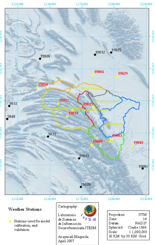
(61) 50 Figure 5.2 shows the location of the weather stations in the watershed and it can help to explain the variation among the rainfall records. Dominant winds coming from the Gulf of Mexico (east) hit the mountains and most of the rainfall is concentrated in the east face of the mountain range. Stations in the west of the study area are isolated by the mountains and the rainfall amount is smaller. In Figure 5.1, the rainfall of any of the years graphed shows this behavior. For example, the rainfall in station 19003 (east of the watershed) is always greater compared to rainfall in station 19054 (west of the watershed)..

(62) 51. Figure 5.1 Rainfall data for all weather stations in the studied watershed in years A) 1974, B) 1975, C) 1998, and D) 1999..

(63) 52. Figure 5.2 Location of weather stations in study area. Stations in yellow were used for rainfall calibration and validation. All of the stations were used as rainfall input to produce results for years 1974, 1998 and 2020..