Clustering of Cases from Di erent Subtypes of Breast Cancer Using a Hop eld Network Built from Multi omic Data

(1)

Costa Rica Institute of Technology

School of Computing

Master’s Program in Computing

Clustering of Cases from Different Subtypes of Breast Cancer Using

a Hopfield Network Built from Multi-omic Data

Thesis submitted to the School of Computing, to opt for the degree of Magister Scientiae in Computing,

with emphasis in Computer Science

Olger Calder´

on Ach´ıo

Student

Dr. rer. nat. Francisco Siles Canales

Thesis Adviser

(2)

(3)

(4)

Dedication

To my parents and brother, who remained by my side from beginning to end and whose support was always unconditional.

(5)

Acknowledgements

I would like to thank Dr. Francisco Siles, my thesis advisor and director of the Pattern Recognition and Intelligent Systems Laboratory, for his constant reminder of “persevering under pressure”. This phrase has a personal and special meaning for both of us.

I am grateful to Dr. Esteban Meneses from the National Advanced Computing Collaboratory (CNCA) and Dr. Rodrigo Mora from the Tumoral Chemosensibility Laboratory (LQT), who showed interest in my research and made me feel like a colleague of theirs. Hope this collaboration might not be the last one.

A very special gratitude goes out to the members of the PRIS-Lab (specially those of BEND team) who made me feel part of a greater research initiative. Tackling complex problems like cancer does not sound that scary alongside them.

And finally, last but by no means least, to the colleagues at Mobilize who identified with me and supported my goals in one way or another. Special mention to Diego P´erez for being the best working partner at the master’s program. My gratitude towards Carlos Bastos, Olman Garc´ıa, Ivan Sanabria and Hugo Fern´andez for their comprehension along the way.

(6)

Epigraph

The results suggest a helical structure.

Rosalind Franklin, Lecture Notes (November 1951)

(7)

Abstract

Despite scientific advances, breast cancer still constitutes a worldwide major cause of death among women. Given the great heterogeneity between cases, distinct classification schemes have emerged. The intrinsic molecular subtype classification (luminal A, luminal B, HER2-enriched and basal-like) accounts for the molecular characteristics and prognosis of tumors, which provides valuable input for taking optimal treatment actions. Also, recent advance-ments in molecular biology have provided scientists with high quality and diversity of omic-like data, opening up the possibility of creating computational models for improving and validating current subtyping systems. On this study, a Hopfield Network model for breast cancer subtyping and characterization was created using data from The Cancer Genome Atlas repository. Novel aspects include the usage of the network as a clustering mechanism and the integrated use of several molecular types of data (gene mRNA expression, miRNA expression and copy number variation). The results showed clustering capabilities for the network, but even so, trying to derive a biological model from a Hopfield Network might be difficult given the mirror attractor phenomena (every cluster might end up with an op-posite). As a methodological aspect, Hopfield was compared with kmeans and OPTICS clustering algorithms. The last one, surprisingly, hints at the possibility of creating a high precision model that differentiates between luminal, HER2-enriched and basal samples us-ing only 10 genes. The normalization procedure of dividus-ing gene expression values by their corresponding gene copy number appears to have contributed to the results. This opens up the possibility of exploring these kind of prediction models for implementing diagnostic tests at a lower cost.

Index Terms - Breast Cancer, Neural Networks, Machine Learning, Pattern Recognition, Biocomputing.

(8)

Resumen

A pesar de los avances cient´ıficos, el cáncer de mama todav´ıa constituye una de las principales causas de muerte entre las mujeres en todo el mundo. Dada la gran heterogeneidad entre los casos, han surgido distintos esquemas de clasificación. La clasificación intr´ınseca de subtipos moleculares (luminal A, luminal B, HER2-enriquecido y tipo basal) toma en cuenta las carac-ter´ısticas moleculares y el pronóstico de los tumores, lo que proporciona información valiosa para realizar acciones de tratamiento óptimas. Además, los recientes avances en biolog´ıa molecular han proporcionado a los cient´ıficos alta calidad y diversidad de datos ómicos, lo que abre la posibilidad de crear modelos computacionales para mejorar y validar los sistemas de subtipos actuales. En este estudio, se creó un modelo de Red de Hopfield para el subtipo y la caracterización del cáncer de mama utilizando datos del repositorio “The Cancer Genome Atlas”. Aspectos novedosos incluyen el uso de la red como un mecanismo de agrupación y el uso integrado de varios tipos de datos moleculares (expresión genénica de ARNm, ex-presión de miARN y variación del número de copias). Los resultados mostraron capacidades de agrupamiento para la red, pero aun as´ı, tratar de derivar un modelo biológico de una Red de Hopfield podr´ıa ser dif´ıcil dado el fenómeno de los atractores espejo (cada grupo podr´ıa terminar con un opuesto). Como aspecto metodológico, se comparó a Hopfield con los algoritmos de agrupamiento kmeans y OPTICS. El último, sorprendentemente, sugiere la posibilidad de crear un modelo de alta precisión que diferencie entre muestras luminales, enriquecidas con HER2 y basales usando solo 10 genes. El procedimiento de normalización de dividir los valores de expresión génica entre su número de copia de gen correspondiente parece haber contribuido a los resultados. Esto abre la posibilidad de explorar este tipo de modelos de predicción para implementar pruebas de diagnóstico a un costo menor.

Palabras Clave- Cáncer de Mama, Redes Neuronales, Aprendizaje de Máquinas, Reconocimiento de Patrones, Biocomputación.

(9)

Chapter 1 Introduction

1.1 Overview

Cancer is a complex disease of molecular basis with a high mortality rate. Given the great heterogeneity between cancer cases in terms of genetic behavior and prognosis, some authors prefer to think of “cancer” as a group of related diseases instead of a single pathological condition [29, 6, 16]. Such molecular diversity is even present on tumors originating from the same tissue. For example, breast cancer it is now known to have different molecular subtypes which the community has agreed upon, namely luminal A, luminal B, HER2-enriched and basal-like [44, 7]. Current classification schemes will rarely stay static as new studies might reveal finer-grained classifications for cancer subtypes. Better characterization of these subtypes at the molecular level will lead to the improvement of diagnostics and treatments.

Recent advancements in molecular biology have provided scientists with high quality and high diversity of omic-like data product of processes like sequencing, transcriptome profiling, copy number quantification and methylation profiling. This has opened the door to new types of studies which make use of computational models built upon this data. Such models look to capture patterns in data so our understanding in cancer dynamics can be improved. Sub-cancer classification has benefited from these approaches, specially from unsupervised learning techniques like clustering which has revealed the existence of novel cancer subtypes [43]. There is still room left for trying novel approaches in this regard, specially when making use of non-conventional clustering algorithms and of data integration techniques for different molecular data types, which overall, have showed promising results [38, 43].

An unsupervised learning neural network named Hopfield Network has just recently begun to be explored to model energy landscapes of cellular differentiation [41, 22, 13, 34, 12]. After being trained with samples data, this model generates a landscape with attractor states which

(13)

1.1. OVERVIEW 13 likely correspond to stable phenotypic states of cellular development, in a manner similar as Waddington Epigenetic Landscape does [13]. The states could describe either specialized healthy cells configurations (e.g: epithelial cells, neurons, blood cells), or diseases states as the different cancer subtypes [22, 13]. Although already been used to explore clustering of gene expression profiles into cancer subtypes [22], so far, the technique has not yielded a high quality characterization of breast cancer according to its molecular subtypes (luminal A, luminal B, HER2-enriched and basal-like). Also the training of these models has been strictly limited to using gene expression quantification data from microarrays.

On this study, it was explored if it was possible to create a Hopfield Network model for breast cancer subtyping and characterization. Several types of omic data from samples of The Cancer Genome Atlas were taken into disposition so different data integration strategies could be tested. While the initial expectation of finding finer subtypes aside from those exposed in the literature was rapidly turned down, the model showed capabilities for being used for clustering purposes. Still, some of its appealing features like the attractors landscape model should be accompanied of careful interpretation, as it might expose characteristics that make little sense under a biological context.

As a methodological aspect, Hopfield was compared against other clustering methods like kmeans and OPTICS (a density-based algorithm similar to dbscan). The last one, in a kind of unexpected way, showed the possibility of creating a high precision model that differentiates between luminal, HER2-enriched and basal samples using only a few genes. This opens up the possibility of exploring these kind of models for implementing diagnostic tests at a lower cost.

The present thesis document is composed of the following chapters:

• Chapter 1 serves as an introduction to the research problem at hand. Also, the con-tributions and objectives of this work are stated.

• Chapter 2 contains a theoretical framework with concepts relevant to both the research problem and applied methods.

• Chapter 3 describes most of the methodological aspects that were followed in order to fulfill the objectives.

• Chapter 4 shows and discusses the results obtained through experimentation.

(14)

1.2 Background and Related Work

1.2.1 Cancer Statistics

According to a study published by the American Medical Association, in the year 2015, it was estimated that 17.5 million cancer cases were diagnosed globally, and there were 8.7 million reported deaths [14]. It was the leading second cause of death behind cardiovascular diseases. Between 2005 and 2015, incidence of cancer increased by 33% due to factors like population growth and aging. These statistics reflect the need to invest in cancer control planning and prevention. This also calls for the development of accurate diagnostics, so patients can be treated in the most effective way for the particular cancer type/subtype they have.

In 2015, it is estimated that 2.4 million cases of breast cancer occurred and it was the cause of death for 523.000 women and 10.000 men [14]. In the context of Costa Rica and according to the Ministry of Health, in year 2010, breast cancer occupied the first place on mortality by cancer on women, followed by stomach, colon and cervix cancer [8].

1.2.2 Repositories of Molecular Data

In the latest years there have been great advancements in the bioinformatics community in terms of production of molecular data and available repositories.

The Gene Expression Omnibus is a public functional genomics data repository supporting data submissions, mainly gene expression profiles [11]. The Cancer Cell Line Encyclopedia (CCLE) provides detailed genetic characterization of human cancer cell lines including access to DNA copy number, gene expression and mutation data [3]. It also includes chemosensi-tivity responses for several anticancer drugs. The GenBank, the National Institute of Health (NIH) database of DNA sequences, is constantly being updated with annotated samples and makes a release every two months [4]. These public repositories bring new opportunities, encouraging the use of shared resources and scientific reproducibility.

(15)

1.2. BACKGROUND AND RELATED WORK 15 Just recently, the TCGA was integrated into a bigger initiative named Genomic Data Com-mons (GDC) [28]. The GDC mainly integrates two repositories: the TCGA and the Thera-peutically Applicable Research to Generate Effective Therapies database (TARGET)1. Both databases have been harmonized under the same set of bioinformatics tools, opening the possibility of establishing comparisons between the two repositories of data. It is expected that new data will be imported to the GDC.

1.2.3 Clustering Gene Expression Patterns

The clustering of gene expression patterns from microarrays has been of special interest in the community. It opens up the door for gaining insights on gene co-regulation, and disease characterization as well [19]. New cancer types have been discovered and studied on this way.

Pioneering studies on this problem include [15] and [1]. On the former it was possible to discover the subtypes of acute myeloid leukemia (AML) and acute lymphoblastic leukemia (ALL) without prior knowledge using self-organizing maps (SOMs). In the second one, distinct types of diffuse large B-cell lymphoma were identified.

Average-linkage hierarchical clustering was used in [39], on gene expression patterns of breast cancer derived from cDNA microarrays. It was found that at least two distinct groups inside luminal type of cancer existed with characteristic gene expression profiles and different prognosis. The classification of luminal into A and B subtypes appears to initially come from this study.

There have been also comparative studies of the efficiency of several clustering algorithms under the context of gene expression clustering.

On [19], authors make note of the complexities associated with gene expression datasets like the high dimensionality and noise problems. The authors argue that agglomerative and partitive clustering techniques tend to fall short because of these aspects, and remark bi-clustering algorithms as an appealing option. An important discussion point is that clustering methods that don’t need to specify an initial K (number of desired clusters) have an advantage in terms of exploration without a priori knowledge. But even if they don’t need to specify K, some of them calculate thresholds for dividing the clusters which might make little sense in the biological context.

Souto et al performed a comparative study of seven clustering methods and four proximity measures for the analysis of 35 cancer gene expression microarray datasets [9]. The authors contributed with a large-scale evaluation which included other clustering methods aside from the “classic” ones like hierarchical clustering. The evaluated methods included:

(16)

cal clustering with single, complete, and average linkage, k-means, mixture of multivariate Gaussians, spectral clustering and nearest neighbor-based method. It was found that the finite mixture of Gaussians and k-means gave the best results in terms of revealing the true structure of the datasets. The authors also note that most of bioinformatics studies involving clustering make use of hierarchical clustering, probably because of factors like ease of use and available implementations.

Pirooznia et al compared the efficiency of several classification and clustering algorithms [32] making use of eight microarray cancer datasets. The evaluated clustering algorithms were: k-means, density-based clustering, farthest first traversal algorithm and expectation maximization clustering. Authors reported that the choice of feature selection method, the number of genes in the gene list, the number of cases (samples) and the noise in the dataset all influence the quality of the results. Farthest first traversal algorithm obtained the greatest accuracy.

Hopfield Networks just recently began to be used for clustering cancer samples into cancer subtypes by Maetschke et al [22].

Overall, most studies have been carried out with microarray data (vs RNA-Seq), non-neural networks algorithms and the number of used samples rarely overpass 100.

1.2.4 Hopfield Networks Usage in Gene Expression Landscapes

Hopfield Networks (HNs), recurrent neural networks that model associative memory [17, 23], have been used before to model attractor landscapes from gene expression data. The main idea has been to construct models that have the capacity of mirroring the dynamics of the underlying gene regulatory network when converging towards a certain stable state from the cell. Computing units in the network correspond to genes, and the weights between units represent how much the expression of genes affect each other.

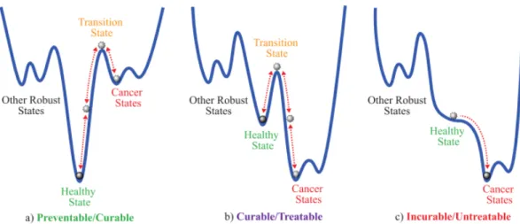
The gene expression levels from a cell tend to converge to stable states of minimum energy as the cell differentiates into more specialized states [49] (see figure 1.1). In the same way, a HN can associate an input pattern with the most resembling stored pattern, hence converging in some way.

(17)

1.2. BACKGROUND AND RELATED WORK 17

Figure 1.1: After being trained, a Hopfield Network can be used to model an energy landscape of cellular differentiation. Attractor states (stored patterns) at the bottom of the landscape correspond to stable phenotypic cell configurations of minimum energy (gene expression levels that induce the cell to either healthy or disease states). Transition states could be also present at peaks or as local minima. Source of image: [49].

Szedlak et al explored the asymmetric Hopfield model for generating attractor states for cancer gene expression data [41]. Once trained, the authors proposed an analysis on the network’s weighted graph for detecting strongly connected cluster of nodes that have a significant impact on signaling in the gene network. In this way, candidate sets of proteins can be detected for intelligent therapeutic interventions.

Koulakov and Lazebnik used Hopfield Networks to support a model for cell fusion [21]. Each cell has a Hopfield Network with several attractors, each one corresponding to a stable cell phenotype. The fusion of two different cells might give rise to spurious attractor states which might turn the cell cancerous.

Pusuluri et al also study [34, 33] how recurrent neural networks can be used to model energy landscapes of biological processes with a given set of attractors. He puts particular attention to the properties of the generated landscapes instead of concentrating on other previously analyzed aspects of the networks like storage capacity and stability of patterns. Hopfield networks, and a similar model (Kanter and Sompolinsky) were used in the study.

1.2.5 Clustering Cases from Subtypes of Breast Cancer

(18)

population-based study, giving as a result two major subgroups based on their ER status [40]. It correlated well with basal and luminal characteristics.

A comprehensive study using different data platforms from The Cancer Genome Atlas rein-forces the fact that the four breast molecular subtypes (luminal A, luminal B, HER2-enriched and basal-like) are well established [44] and each possesses their own characteristics for each of the molecular subtypes. The authors claims that this reinforces the hypothesis that much of the clinically observable heterogeneity occurs within these major subtypes.

In [43] known breast cancer subgroups were detected. The authors made use of an integrated data approach of four platforms (gene messenger RNA expression, DNA-methylation, copy-number variation and microRNA expression) and clustered cases of 4,434 samples from The Cancer Genome Atlas across 19 cancer types. The technique involved the selection of prin-cipal components from each data type and then an early (concatenation-based) integration of data was performed. Then DBSCAN (Density-Based Algorithm for Discovering Clus-ters) was applied. Subtype analysis of the 563 breast cancer cases revealed five clusters that mostly correspond to the know molecular subtypes. However luminal A was splitted into two different clusters and some cases of basal-type were put together with the ones of HER2-type into a single cluster. See figure 1.2. This thesis work took a different approach for data integration, although it used the same molecular data types (except methylation values).

Figure 1.2: Clustering results from [43]. The method managed to divide luminal A cases into two clusters, but was unable to correctly separate HER2-type cases from basal.

(19)

1.3. PROBLEM DEFINITION 19 objectives and methodology. They suggested using Hopfield Networks specifically for char-acterizing cancer subtypes as attractor states in a Hopfield Network. They also introduced a pruning method for discarding genes which would contribute little to the overall perfor-mance of the model. The authors used the microarray datasets proposed by Wang et al [47] and Souto et al [9] for training the networks. The ones that were trained using breast cancer datasets did not particularly show good results. This work differs in the sense that was specifically aimed at breast cancer characterization and contemplated using several omic types (not just gene mRNA expression) for improving the accuracy of the model. Used data was from the TCGA and, for validation purposes, prelabeled using the four main molecular subtypes of breast cancer.

1.3 Problem Definition

From the biological point of view, breast cancer heterogeneity constitutes the main prob-lem. Aspects like diagnostics, prognosis and effectiveness of treatments are all affected by the molecular characteristics of tumors. This problem can be approached by building a computational model of breast cancer subtyping.

Given a dataset D with multi-omic data of n cancer samples, the problem of building a model for cancer subtyping can be formally defined as a type of clustering problem.

A clustering C for D is a partition of the n patients into mutually disjoint subsets C1, C2,

. . .,CK called clusters. Formally the following properties must hold [25]:

C ={C1, C2, . . . , CK}, Ck1 ∩Ck2 =∅with k1, k2 ∈ {1, . . . , K}, k1 6=k2 and

There is a function subtype : D → L which associates a patient with a label for his/her cancer subtype. L = {l1, l2, . . . , lm} is the set of possible labels known a priori for each known cancer subtype. In the context of breast cancer this set corresponds to:

L={luminalA,luminalB,basal,her2}

.

(20)

A reference clusteringC0 can be defined asC0 ={C₁0, C₂0, . . . , C_m0 }. Each clusterC_k0 is defined as C_k0 ={pi ∈D, i∈ {1, . . . , n}|subtype(pi) = lk}.

There is also a numerical function f that quantifies how much two clusterings differ accord-ing to some criteria. The problem consists in findaccord-ing a clusteraccord-ing C such that f(C, C0) is optimized as much as possible. The function f chosen for this study was the Adjusted Rand Index (ARI) which ranges from -1 to 1. Higher values denote better agreement between the clusterings in terms of precision and recall.

From the statistical point of view, the problem can be seen as a multivariate analysis where thousands of variables (in this case transcript levels of genes) are involved per observation, and there is also the possibility of using other data views like copy number variation for deriving new features.

1.4 Hypothesis

Through the use of multi-omic data from the TCGA and a hebbian learning scheme, is possible to create a Hopfield Network model for breast cancer subtyping and characterization. This model will either differentiate between the main four molecular subtypes of breast cancer, or will find a finer classification inside these.

1.5 Justification

Under this context, having a computational model that accurately clusters patient cases would help in the characterization and discovery of subtypes of breast cancer. Hopfield Networks serve well both purposes. After being trained, each attractor state in the net-work encodes a binary state for each gene of interest (+1 for an highly expressed gene, -1 otherwise). An attractor defines a cluster for those cases that are converging to it.

Characterization means that key regulator genes and the dynamics between them could be better understood for each detected subtype (cluster) in the model. In other words, the attractor states of the model could aid in the identification of candidate biomarkers for prog-nosis and treatment, as such states would encode the different breast cancer configurations for the gene regulatory network. The candidate biomarkers would need to be validated later in vitro by experts in the area.

(21)

1.5. JUSTIFICATION 21 attractor states where a certain subtype of breast cancer cases are concentrated (e.g basal-like cases), might reveal a finer subdivision inside the subtype. This could be later validated using tools like survival analysis, which might reveal significant differences for the prognosis of the subtypes.

If compared to other classical approaches for clustering, there are a number of reasons why using Hopfield Networks represents an innovative and appealing option:

• Biological interpretation: Hopfield Networks associative memory capabilities can be used to model an energy landscape with attractor states of minimum energy at the bottom. The landscape metaphor has been used before by the biological community, specially when referring to the cellular differentiation process and the progression of diseases [49]. The cell’s gene regulatory network, when adjusting the levels of tran-scripts of genes, highly resembles a dynamical system that seeks to converge to a stable state as time passes. Hopfield Networks, when recalling a stored pattern mimic exactly this behavior, as the input pattern converges to the state of the nearest attractor in the landscape.

• No need of prior knowledge: Hopfield Networks don’t need an initial k number of clusters. Attractors are discovered based on the characteristics of the training data. This proves to be useful when looking for potential new cancer subtypes.

• An unified clustering-classification framework: Hopfield Networks separate the learning process (adjusting the weights of links between units) from the recalling pro-cess (associating an input with a stored attractor). The recalling propro-cess is first effectu-ated on the training samples for clustering purposes. Then when the genereffectu-ated model is validated and understood, recalling could be used on new samples for classification purposes.

• Algorithmically simple: The coding effort for implementing a Hopfield Network is not high. Between 35 and 50 lines of code are needed in a language like R which is optimized for data manipulation.

• Other analysis: It is possible to use visualization methods like the one in [22] for displaying the energy landscape associated with the network. This intuitively gives a measure of how far are cases from converging to their associated attractors. It is also possible to trace the convergence route from each case to their attractor, hence revealing the evolution of the gene regulatory network as it converges to a stable state [12]. Other properties of the attractors like their basin of attraction and density have been studied [33].

This study introduced some novel aspects from the methodological standpoint:

(22)

involving Hopfield Networks are not fully focused on breast cancer and use other simpler classification schemes for validation.

• Testing new multi-omic approaches for data integration using three different views of data: gene (mRNA) expression, miRNA expression and copy number variation. Most studies are limited to the usage of gene (mRNA) expression only.

• A high quantity of cases from The Cancer Genome Atlas was used (around 1000). Most studies limit to smaller datasets (100 cases at most).

Other factors that also motivated and contributed to this research effort are the proliferation of data science techniques, the improvement of latest generation genomic and sequencing technologies and the collaborative effort that is being held by the PRIS-Lab2 and the LQT3, which played a key role for this project’s definition and development.

The PRIS-Lab BEND team, in collaboration with other laboratories or research centers, is fully devoted to research on the field of Computational Biology. Research interests include: cell tracking on light field microscopy, chemosensitivity prediction, computational structural molecular biology, recognition of patterns in optical spectroscopy, among others. According to the National Institute of Health, the field of Computational Biology seeks to use math-ematical and computational methods to answer theoretical and experimental questions in the sciences of life, in contrast with Bioinformatics which is more concerned about using informatics principles to make biological data more understandable and useful [30].

1.6 Objectives

1.6.1 Main Objective

Use a Hopfield Network model built from multi-omic data of the TCGA for clustering cases from different subtypes of breast cancer.

1.6.2 Specific Objectives

1. Create the necessary software infrastructure for loading and preprocessing the data from the TCGA.

2. Create the necessary software infrastructure for training and visualizing a Hopfield model.

2_{Pattern Recognition and Intelligent Systems Laboratory, School of Electrical Engineering, University of}

Costa Rica.

(23)

1.6. OBJECTIVES 23 3. Design and implement procedures for generating either standalone4_{or integrated datasets}

that make use of the gene (mRNA) expression, miRNA expression and copy number variation data views.

4. Run experiments varying the generated datasets, measure the effectiveness of the trained models (while comparing with at least two other algorithms) and analyze the results.

1.6.3 Scope

• The used data integration approaches were “early”. This means new datasets were derived before performing the training procedure.

• Feature selection played a crucial role as the total number of features exceeded the 60000. Only protein coding genes were used and not more than 100 were chosen for creating a model.

• Even if the proposed approach for training the Hopfield model was general enough to be applied to data of other cancer types, the study was exclusively focused on breast cancer cases from the TCGA.

• Cases from the TCGA that did not have all the necessary data views (gene mRNA expression, miRNA expression, copy number variation) were excluded from the study.

• Having an initial subcancer PAM50 label for the used cases is a prerequisite condi-tion for validating the created model. Otherwise, cases which did not possess this information were excluded from the study.

• It was not contemplated in the scope of the study creating a R package or similar.

• All analysis were executed in silico.

1.6.4 Deliverables

The following table describes all the deliverables for this project. Please refer to the specific objectives enumerated in the previous section.

(24)

Objective Activities Deliverable(s) Specific Objective

1

Implement functions in R. Source code in R for loading and preprocessing the data from the TCGA.

Specific Objective 2

Implement functions in R. Source code in R for train-ing and visualiztrain-ing a Hop-field model.

Define and implement procedures for generating either standalone or inte-grated datasets.

Source code in R for creat-ing the datasets.

Run experiments and collect results data.

(25)

Chapter 2 Theoretical Framework

2.1 The Problem of Cancer

Cancer has been a mainstream human race health problem for years. It mainly causes an erratic behavior on the cell natural mechanisms of division and programmed death (apopto-sis), which in turn triggers abnormal cell growth and proliferation through the tissues [29]. This process gives rise to the formation and development of masses of cells called tumors. It might prove lethal, specially if these enter an advanced state where they spread towards other organs different from the one of origin, a process called metastasis.

Carcinogenesis, the process of cancer formation, is mainly the result of mutations in somatic cells1. Some cancer-causing mutations are due to environmental factors and exposure to carcinogenic substances. Others are the result of errors during DNA replication and lack of proper DNA repairing processes. Given its genetic nature, the susceptibility to develop cancer varies from person to person. Cells can also become cancerous by being infected by certain viruses (called oncoviruses).

When a cell becomes cancerous, the gene expression levels of certain genes become altered and differ from that of a normal (differentiated) cell. There are mainly 2 types of genes that affect cancer. Oncogenes and tumor-suppressor genes [18, 16]. Oncogenes are mutated forms of certain genes that usually play some role in cell division or growth. By themselves, these genes (called proto-oncogenes in their normal forms), are necessary for the correct functioning of the cell. However, in their oncogene forms, they are cancer-producing agents. This is normally reflected in terms of proteins with hyperactive behaviors or overproduction of proteins associated with the oncogenes. Proto-oncogenes usually code for: growth factors, cell surface receptors, transcription factors and signal transmission proteins (like kinases).

1_{Cancer could start by other means like the silencing of key genes product of epigenetic modifications}

like methylation [42].

(26)

On other hand, tumor-suppressor genes usually suppress uncontrolled cell division. They have a protective function, that when inactivated via mutations, might give rise to tumors. It is usually necessary the combination of mutations on both oncogenes and tumor-suppressor genes to give rise to cancer. Given the important role they play, some oncogenes are used as biomarkers or are targeted by drugs to inhibit cancer progression.

Several molecular processes also contribute to carcinogenesis or irregularities in the gene expression levels of cancer cells:

• Modifications of the karyotype (number and appearance of the cell chromosomes), might lead the cell to an aneuploid state which contributes to cancer progression [37]. Some regions (or even complete chromosomes) might be copied or deleted.

• Expression of miRNAs play a regulatory role for other genes [31]. The miRNAs are a type of small non-coding RNAs that bind to the transcripts of other genes, thus preventing their translation to proteins.

• Methylation is an epigenetic process that also plays a role silencing certain key genes [42]. Tumor-suppressor genes might be affected in this way.

Cancer types can be classified by tissue of origin, e.g. stomach, colon, breast, among others. But finer classifications could exist inside these types.

2.2 Breast Cancer Classification

Breast cancer develops from breast tissue. Breast tissue includes the one from the lobules (glands that make milk), the ducts (thin tubes that carry the milk from the lobules to the nipples), lymph nodes and blood vessels. Breast cancer usually originates from the tissue of the ducts (ductal carcinoma) or from the lobules (lobular carcinoma), but could also originate from other places. If the abnormal cells haven’t spread to neighboring tissues, then it is said that the cancer is in situ. Otherwise it is called breast invasive carcinoma [27]. Breast cancer is the most common cancer on woman. It is estimated that it affects about 12% women worldwide [24].

Breast cancers can be categorized using a variety of criteria. Every one of them provides some input that can be used by oncologist to determine the best course of action when treating a patient:

(27)

2.2. BREAST CANCER CLASSIFICATION 27 and lobular carcinoma (depending of the primary site of the tumor). Tumors in the same histopathological category can follow different clinical courses and show different responses to the same therapy [15, 6]. This reveals the necessity of other means of classification.

2. Grade: indicates how much have cancer cells lose their differentiated state in com-parison to normal cells of the tissue. Common descriptions are well differentiated (low-grade), moderately differentiated (intermediate-grade) and poorly differentiated (high-grade). The higher the grade, the worse the prognosis. It is also expected that higher grade tumors will differ in a greater way from normal cells in their gene expres-sion levels.

3. Stage: the relative size of the tumor and how much has spread to neighboring tissues. Stage 0 refers to in situ state (benign tumor). Stages 1-3 indicate an invasive state and the higher the number, the greater the size of the tumor and dispersion within the breast or lymph nodes. Stage 4 indicates metastatic state. Again, higher numbers have associated a less favorable prognosis.

4. Receptor status: in breast cancer cells there are 3 receptors of particular importance: estrogen receptor (ER), progesterone receptor (PR) and human epidermal growth fac-tor recepfac-tor 2 (HER2). Their presence or absence is currently an important input for deciding the most appropriate therapy. For example, estrogen receptor positive cancer cells (ER+) need estrogen in order to growth, so they can be treated in a way that specifically target estrogen levels. Triple negative cancers (ER-/PR-/HER2-) currently have the worse prognosis because of the lack of targeted treatments.

5. Molecular subtypes: these types give an insight into the receptor status along with tumor grade and prognosis [20]. Novel approaches might categorize cases into one of the 4 main classes:

• Luminal A: Tend to be estrogen receptor-positive (ER+), HER2 receptor-negative (HER2-) and tumor grade 1 or 2. They also tend to have the best prognosis and can be treated with hormone therapy. Most breast tumors are Luminal A.

• Luminal B: Tend to be estrogen receptor-positive (ER+), may be HER2 negative or positive (HER2-/HER2+). Have poorer prognosis than luminal A reflected in aspects like a higher grade and stage.

• Basal-like: The majority of these cases are triple negative (ER-/PR-/HER2-). Of all subtypes, these have the poorer prognosis and tend to be aggressive. These are usually treated with surgery, radiation therapy and chemotherapy.

• HER2-enriched: Most of them (70%) are HER2+. These also tend to be ER- and PR- and have a poorer tumor grade. HER2 type breast cancers can be treated with anti-HER2 drugs like trastuzumab (Herceptin).

(28)

2.3 Pattern Recognition and Artificial Neural Networks

Pattern recognition is the act of taking in raw data and taking an action based on the category of that pattern [10]. A common pipeline followed on the Pattern Recognition paradigm involves the steps of data preprocessing, feature extraction, and then, classification (usually performed by some previously trained model). A lot of other challenges and sub-problems are usually present when building pattern recognition systems, among these: noise in the data, overfitting, high dimensionality, use of prior knowledge, missing features and others.

If the samples from the training data possess labels that are used by the learning algorithm then the process is said to be supervised. Otherwise it is said to be unsupervised. Unsuper-vised learning is popular for performing exploratory data analysis where a clear structure of data is not known beforehand. It serves well for finding candidate categories for the data and identifying features of interest [10]. Major departures from expected characteristics (like the discovery of subclasses) can be found when using unsupervised learning methods.

Clustering is probably the most common task under unsupervised learning. The idea behind consists of finding a partition of a set of entities, such that similar ones are combined in the same clusters, while dissimilar entities end up on different clusters [26]. The concept of similarity might vary entirely from one clustering algorithm/methodology to another. Hence, the problem of finding the best clustering algorithm for a given problem is not straightforward.

Artificial neural networks are computing systems that seek to mimic the computational capabilities present in the biological neurons [36]. These systems are used for both supervised and unsupervised learning tasks. An artificial neural network has a collection of connected computation units. These connections (usually weighted) mark the directionality of signals between computing units. If the amount of input signal overpass some threshold, then the given unit triggers a signal that is sent to other connected units. Flows of signals in this fashion (along with the correct weights between units) allow the computation of functions. Learning a function with an artificial network usually involves adjusting these weights.

One of the categorizations used for artificial neural networks takes into account how the computation units are connected. The most common type, feed-forward neural networks don’t posses cycles between units and their connections. On the other hand, recurrent neural networks might have connections between units that form cycles.

2.4 Hopfield Networks

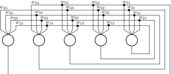
A Hopfield network is a type of recurrent neural network with n computing units, where n

(29)

2.4. HOPFIELD NETWORKS 29 output unit, which results in a matrixW of approximately n2_/_{2 weighted links representing} the network (basically, a complete undirected graph). See figure 2.1.

Figure 2.1: A Hopfield Network is a full, undirected graph. In other words the weightwnmis equal to the weight wmn. This property is necessary for the network to converge to a stable state when “recalling” a stored pattern from a input pattern.

Two popular approaches for calculating the weights between links are Hebbian learning and Pearson correlation indexes. The network can be trained using Hebbian learning with the following formula:

Here, m is the number of patterns used to train the network. The formula calculates the sum over the outer products of the pattern vectors pk, then normalizes values and sets the diagonal with zero values. The result, the matrix W, contains the numerical values of the network links, where Wij is the weight of link connecting computing unit i to computing unit j.

On the other hand. It is possible calculate the weights of the matrixW as Pearson correlation indexes. The entry Wij corresponds to the Pearson correlation index between the values of feature i with that of feature j.

After being trained, the network can be used to “recall”. This means that given a new input pattern p, the network can associate the pattern p with the closest pattern q that it remembers. This ability to reconstruct stored patterns from similar input is the reason Hopfield networks are considered a way of implementing associative memory. Input patterns associated with the same stored pattern form a cluster of similar entities.

(30)

time steps t. At any time step t0, each computing unit has a binary state si ∈ {−1,1},

i∈1, . . . , n. The states for the next time step are calculated as follows:

s(_it0+1) =sgn

n

X

j

Wijs (t0₎

i

!

(2.2)

The sgn is defined in the following way:

sgn(x) =

(

+1 x >0

−1 x≤0 (2.3)

Given an input patternp= (p1, . . . , pn) for the “recall” phase, the initial state of the network is calculated as s0 _{= (}_sgn₍_p

1), . . . , sgn(pn)). Then, equation 2.2 is run for the t iterations. It is guaranteed that if t→ ∞, then the state of the network will converge to a stable state with minimum energy.

(31)

Chapter 3 Methods

The present chapter purpose is to fully describe the methods that were followed in order to fulfill each one of the specific objectives.

3.1 Computing Platform

As a methodological aspect relevant across all specific objectives, it is stated that the soft-ware platform used for running algorithms, visualizing data and performing analysis was exclusively the R Statistical Computing Environment version 3.4.3 (2017-11-30) – “Kite-Eating Tree”. It is also worth mentioning that the IDE RStudio (Version 1.1.414) was used in order to facilitate the coding process. Its debugging and documentation features were worth exploring and contributed to the development work.

3.1.1 Used Packages

Relevant used R packages1 _{(and their respective versions) are listed below:}

• TCGAbiolinks(2.6.12) -An R/Bioconductor package for integrative analysis with GDC data: Provides facilities for querying and downloading data from the Genomic Data Commons repository. It also includes other convenient features, namely, the capacity of loading downloaded data as R data frames (table-like data structures) and the access to premade datasets with annotation labels for the TCGA patients.

1_{The Bioconductor version used was 3.6. Every}_Bioconductor_{package is also a R package, but it might}

follow a different release cycle that differs from the normal R scheduled releases.

(32)

• CNTools (1.34.0) - Convert segment data into a region by sample matrix to allow for other high level computational analyses: This Bioconductor package allows transforming copy number per segment data to a copy number per gene matrix. This is important in terms of compatibility with other data types, such as expression data which is given in terms of genes (not regions).

• Matrix(1.2-12) -Sparse and Dense Matrix Classes and Methods: This package facilitates more efficient representations and operations for matrix structures than the native ones from R.

• scatterplot3d (0.3-41) - 3D Scatter Plot and rgl (0.99.16) - 3D Visualization Using OpenGL: Used for supporting and enhancing the visualization of data, specif-ically after performing Principal Component Analysis.

• gglot2 (2.2.1) - Create Elegant Data Visualisations Using the Grammar of Graphics: Plotting library for generating the graphics in the “Results” Chapter.

• ClusterR(1.1.1) -Gaussian Mixture Models, K-Means, Mini-Batch-Kmeans and K-Medoids Clustering: Mainly used because it provides functions for calcu-lating clustering validation metrics like Rand Index, Adjusted Rand Index, Precision, Recall, among others.

• dbscan (1.1-2) - Density Based Clustering of Applications with Noise (DB-SCAN) and Related: Contains implementations for the DBSCAN and OPTICS clustering algorithms. OPTICS was used in the experimental runs in order to have a reference point, hence not relying exclusively on the Hopfield Network’s performance for drawing conclusions about multi-omic data usage.

• FactoMineR(1.41) -Multivariate Exploratory Data Analysis and Data Min-ing: Used for its more sophisticated PCA plotting functions.

3.2 Source Code Organization

(33)

3.2. SOURCE CODE ORGANIZATION 33

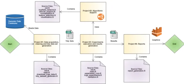
Figure 3.1: Projects organization and dependencies.

3.2.1 Projects

Projects provide the highest level of organization for source code. These reflect the following processes:

1. Data acquisition, cleaning and tidy dataset generation: This project contains all code related to using the GDC client tool for downloading the required data, cleaning it and generating datasets that are ready to be processed by algorithms.

2. Algorithmic support: Contains code implementing machine learning, normalization and feature selection algorithms.

3. Experiments execution and results generation: Provides the infrastructure for running experiments in an efficient and organized way. This project depends on “Algorithmic support” and generates results datasets that act as the input for the “Reports” project.

4. Reports: Generates graphics summarizing the results obtained by previously running the experiments.

As can be seen, these projects constitute a natural organization of code that reflects the pipeline through which data is transmitted from one unit of organization to another. See figure 3.1.

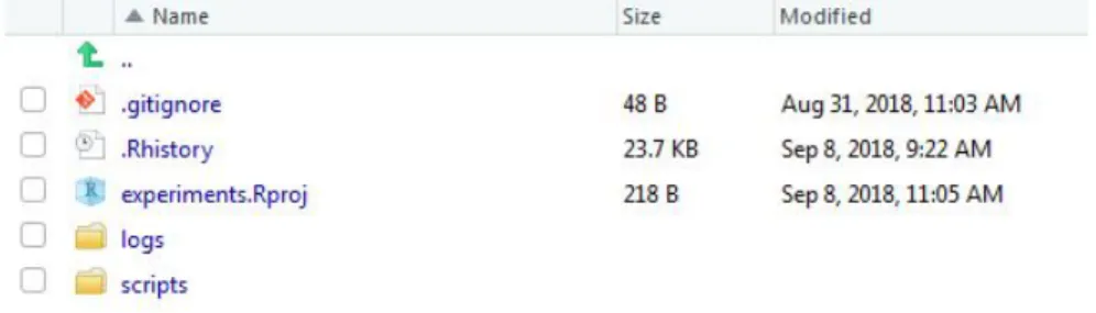
Each project follows the basic folder structure showed on figure 3.2.

(34)

Figure 3.2: Basic project structure. a).Rproj file contains basic configuration for the project. b) logs folder collects the log files generated after the main.R script is executed. c) scripts folder contains all .R files associated with this project. There are two mandatory files on most of the projects: init.R for installing missing package dependencies and main.R which launches the process associated with the project in order to generate the output files. d) A git repository is also defined at this level for source control purposes.

3.3 Data Download and Tidy Dataset Generation

3.3.1 About The Cancer Genome Atlas Data Source

The Cancer Genome Atlas is now part of the Genomic Data Commons project. In summary, the Genomic Data Commons is a property oriented graph database which organizes a great diversity of files. Information could be classified as genomic, clinical or biospecimen depend-ing of its nature. Genomic data categories include: sequencdepend-ing data, copy number variation, DNA methylation, simple nucleotide variation, genomic profiling and transcriptome profiling.

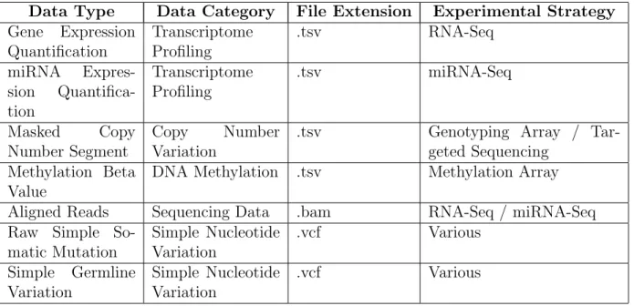
Each data category uses its own data file formats (for example .tsv for transcriptome profiling and .bam for aligned reads). Also each data category can be further subdivided into different data types. Transcriptome profiling has three subtypes e.g: gene (mRNA) expression, exon expression and miRNA expression. For this study three data types for each cancer case were used: gene (mRNA) expression and miRNA expression (both belonging to the transcriptome profiling category), and the masked copy number segment data type (which belongs to the copy number variation category).

Some data categories and types are showed in the table 3.1, just to emphasize the difference between them and the great diversity of multi-omic data available in the Genomic Data Commons repository.

3.3.2 Data Download

(35)

3.3. DATA DOWNLOAD AND TIDY DATASET GENERATION 35 Data Type Data Category File Extension Experimental Strategy Gene Expression

Aligned Reads Sequencing Data .bam RNA-Seq / miRNA-Seq Raw Simple

So-Table 3.1: Examples of data types supported by the6 Genomic Data Commons repository.

1. Using the GDC Data Portal: files to download are selected using a web user interface in a style similar to e-shopping. See https://portal.gdc.cancer.gov/.

2. Using the GDC Data Transfer Tool: a standard client-based mechanism supporting high performance data downloads and submission.

3. Directly consuming a public RESTful API.

The first option was immediately discarded, as some automated way of downloading data is much more preferred over the manual selection of files (at least for the volume intended to be downloaded which summed up to 3000 files approximately). There was one file per data type per patient.

Given that the implementation platform for this project was R, two Bioconductor packages that consume the GDC RESTful API seemed to be good options for downloading and prepro-cessing the necessary data. These were the “TCGABiolinks” and “GenomicDataCommons” packages. The second one is currently maintained by an official member of the National Institute of Health and its API really mirrors the web service structure and the resources it exposes, so it was considered as the first implementation option. However, this package lacked a crucial feature, that was, the capacity of merging all the files for the same data category into a single R dataset.

(36)

After these considerations, the “TCGABiolinks” package was used in conjunction with the GDC Data Transfer Tool (which can be invoked from R). Basically three steps are required by the package to download a group of files and merging them into a single dataset. These are:

1. Create a GDCQuery object with the proper parameters, like in the following example:

GDCquery ( p r o j e c t = ”TCGA−BRCA” ,

data.category = ” T r a n s c r i p t o m e P r o f i l i n g ” , data. t y p e = ”Gene E x p r e s s i o n Q u a n t i f i c a t i o n ” , w o r k f l o w . t y p e = ”HTSeq − FPKM” )

The call to the function GDCquery returns an object containing metadata of the files to download (size, data category and type, among other details) but it does not execute the actual download process. This is useful, as some rechecking can be done, with the possibility of excluding some files from the final download list. The previ-ous query selects cases from the “TCGA-BRCA” (that is Breast Invasive Carcinoma) group, from which it retrieves gene (mRNA) expression quantification files (belonging to the transcriptome profiling category) and which are normalized using the FPKM (Fragments Per Kilobase) procedure [45].

Using raw RNA-Seq reads is not recommended as the gene length (number of base pairs) might introduce a bias. Longer genes capture more reads which does not nec-essarily translate in higher transcription rates [35]. The FPKM normalizes expression rates according to each gene’s length.

2. Call the GDCdownload function with the GDCQuery object:

GDCdownload ( q u e r y = q u e r y . o b j e c t , method = ” c l i e n t ” )

The parameter “method = client” indicates that the “gdc-client.exe” executable is used for performing the download (which can be previously acquired through the GDC’s website). Using the client application is in general a more efficient and robust method for downloading a high quantity of files. The default method uses direct HTTP requests to the REST service which is better suited for a small amount of files.

3. Call the GDCprepare function with the GDCQuery object:

data <− GDCprepare ( q u e r y = q u e r y . o b j e c t , summarizedExperiment = FALSE)

(37)

3.3. DATA DOWNLOAD AND TIDY DATASET GENERATION 37 data type. However all share the same observations (breast cancer patients samples in this case).

The previous process was repeated for each one of the three kinds of genomic data types that were used: gene (mRNA) expression, miRNA expression and masked copy number segment, varying the “GDCQuery” accordingly.

3.3.3 Tidy Dataset Generation

The generated sets still required some extra processing before they are ready to be used. The process of “tidying” refers to cleaning the data from unwanted values and restructuring the observations and variables so they are easy to manipulate [48]. This process is somewhat similar to data normalization on relational databases. Fortunately the tidying process was minimum. This is described in the following sections.

Previous Steps to Generation of Tidy Sets

As a prerequisite to the process of generating the tidy sets for each one of the molecular types used, it was necessary to generate two auxiliary datasets.

1. The first of them contains the breast cancer type labels for each sample, that is the type of breast cancer for each patient (luminal A, luminal B, HER2 or basal). The package “TCGABiolinks” provides a function PanCancerAtlas subtypes that re-turns a predefined dataset with this information. A set of filters were applied to the returned set.

(a) First, filtering the cases to the TCGA-BRCA group of samples.

(b) Second, restricting the type of tissues to solid tumors. This must be deduced from the structure of the TCGA bar codes. These are uniques identifiers used to recognize one sample from another inside the TCGA database. They codify several information pieces separated by hyphen characters. One of these segments indicates the type of tissue. Other type of tissues include “normal-like”, whose most of their cells are still in their normal differentiated states. Some patients have samples for both normal and solid tumor states, but only the latter ones were kept.

(38)

2. The second auxiliary set contains the list of all the protein coding genes. This can be generated by a custom tool (genome browser from the www.ensembl.org website). This set was used for filtering purposes.

Gene (mRNA) Expression Data

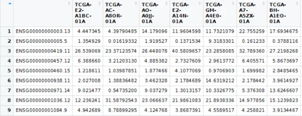
Taking a quick look at how data was organized, it first came to attention that the data appeared to be transposed. That is, patients corresponded to columns and genes to rows. For the ease of treatment it was kept in that way unless some function required the opposite format. This clarification is necessary, as the variables in this study might be referred as the dataset rows (instead of columns) in the following sections. This also applies to the columns, which might be referred as the cases.

For the gene (mRNA) expression data the following changes were applied:

1. Assigning values of the first column to be the “row names” of the dataset. These values corresponded to gene ids as they appear in the Ensembl database. After this, the column was eliminated.

2. Bar codes were cut out to the first 16 characters. The other bar code segments con-tained details that were not useful for the study.

3. Patients for whose breast cancer subtype are not in the “Labels” auxiliary dataset are removed.

4. The second auxiliary set was used to limit the genes to only protein coding genes (around 20000). This constitutes a 3:1 ratio reduction, as the original number of genes is around 60000. The total group of genes include pseudo-genes or genes that produce some kind of non-coding RNA.

See figure 3.3 for the resulting dataset.

miRNA Expression Data

(39)

3.3. DATA DOWNLOAD AND TIDY DATASET GENERATION 39

Figure 3.3: Resulting gene expression dataset which contains Fragments Per Kilobase of transcript per Million mapped reads.

Figure 3.4: Raw miRNA expression data (as generated by GDCPrepare function). Each sample contains three associated columns: read count, read per million miRNA mapped and cross-mapped. Only one sample’s data is showed because of space limi-tations.

1. All columns with raw count values and cross mapped flags were eliminated.

2. The remaining ones were renamed so they only contained the TCGA bar code for the samples.

3. Bar codes were cut out to the first 16 characters.

4. Patients for whose breast cancer subtype are not in the “Labels” auxiliary dataset are removed.

See figure 3.5 for the resulting dataset.

Copy Number Data

(40)

Figure 3.5: Resulting miRNA dataset which only contains read per millions mapped reads values.

Figure 3.6: TCGA copy number segment raw data (as generated byGDCPreparefunction). Sample corresponds to the sample’s barcode which is an unique ID. The Start and End variables denote the base coordinates of the affected region. Segment Mean is a value calculated from the copy number of a region with the formula: log2(copynumber/2), so diploid regions have a segment mean of zero, amplified regions have a positive value and deletions a negative one.

having several records for the same sample, regions containing more than one gene, or genes being split into different regions. See figure 3.6. This format is not suited for high-level analyses like clustering, neither for integration with expression data which uses a matrix of genes by samples. A transformation to such format was necessary in order to perform data integration. Fortunately, the CNTools package provided the means to perform the task.

The R code for generating a reduced segment dataset2 is showed in figure 3.7. First aCNSeg object is created by passing the raw segments.dataset as argument. Then the function getRS does the heavy transformation work. Important arguments are:

1. by: indicates the resulting features, in this case genes.

2. what: value to use when more than one segment includes the same gene. Mean values

2_{This is a term used by the creators of} _CNTools_{, which refers to the resulting dataset that has a single}

(41)

3.3. DATA DOWNLOAD AND TIDY DATASET GENERATION 41 s e g <− CNSeg ( s e g L i s t = segments. d a t a s e t )

rsByGene <− getRS ( s e g , by = ” g e n e ” , what = ”mean” , geneMap = g e n e . map . d a t a s e t )

r e s u l t <− r s ( rsByGene )

write.csv( x = r e s u l t , f i l e = o u t p u t .path)

Figure 3.7: Code for generating a segment reduced set with genes as features for each sample.

Figure 3.8: The resulting gene copy number dataset. Has one value for each sample/gene combination.

were used for this case.

3. geneMap: a dataset that contains the base coordinates and chromosome number for each gene. A custom set was generated using the BioMart online tool using the GRCh38 genome version, which is the same used by the Genomic Data Commons datasets.

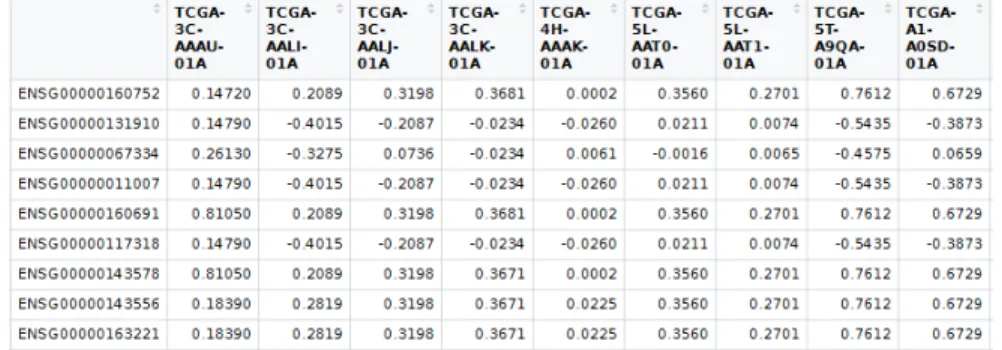
The generated set is extracted using the rs function and then persisted to a .csv file. Still, some cleaning steps similar to those applied to the expression datasets were necessary, namely: reassigning row names, keeping only protein coding genes, modifying barcodes and eliminating unnecessary variables (like base coordinates and chromosome number). After these steps were effectuated, the gene copy number dataset was in tidy form and ready for being used. See figure 3.8.

3.3.4 Extra Normalization Steps

(42)

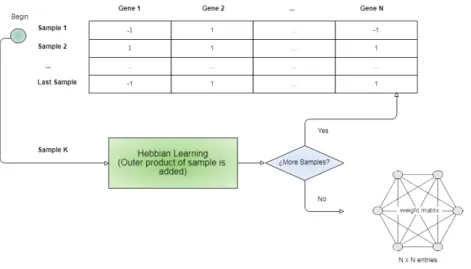
Figure 3.9: High level view of the training procedure.

Both gene (mRNA) and miRNA Expression variables were z-normalized, a step necessary so they could be integrated together under the same data table.

3.4 Implementation and Visualization of Hopfield Model

3.4.1 Training and Recall Procedures

According to the method used by [22], using the Hopfield Network as a clustering procedure requires training the network (using the Hebbian rule) with each sample’s binarized vector3 (whose dimension is equal to the number of used features). Inputs can be binarized using a sign function which assigns 1 to values higher than 0 and -1 otherwise. See the figure 3.9 for a high level view of the training procedure.

Then the recall function is applied to each one of those same vectors, where inputs that converge to the same attractor state are considered to belong to the same cluster. See also figure 3.10.

3.4.2 Implementation Details

For implementation purposes, an example code from the course “Foundations of Neural and Cognitive Modeling” of the University of Amsterdam was used as base4_{. Logic is split into}

3_{In this case the term binarized refers to having only two types of values (not strictly 0 and 1). For the}

present context values are -1 and 1, indeed. Hope this clarification will avoid future misunderstandings.

(43)

3.4. IMPLEMENTATION AND VISUALIZATION OF HOPFIELD MODEL 43

Figure 3.10: High level view of the recall procedure.

two different functions, one for training the network, i.e generating the matrix of weights, and the other for recalling memories (associating inputs with attractor states). Some minor modifications were made to the code. These included:

1. Substituting uses of base matrix R objects with Matrix S4 objects, more suited for higher computation rates and an efficient representation.

2. The outer product of the training equation 2.1 was calculated with the function tcrossprod, which overall is more efficient for this case.

3. The recalling function was modified to add the possibility of tracing convergence routes from the initial vector state to the final attractor state. This is done for visualization purposes and is described below.

The training function is very simple and relies mostly on linear algebra matrix operations. See figure 3.11. The function receives as a parameter a matrix of training inputs called patterns. It is assumed that these patterns are already in a binarized state (only have +1 or -1 values). The number of computing units (or neurons)N is determined by looking at the length of the first input pattern. Then the matrix of weights is initialized with dimensions

N by N, and with a zero on each entry. The sum of outer products is calculated in a loop using the tcrossprod function. As the final steps, entries of the matrix’s diagonal are set to 0 and values are normalized by the number of training patterns so each entry has a value between -1 and 1 (in a manner similar to most correlation coefficients).

(44)

create. h o p f i e l d . network . h e b b i a n <− function( p a t t e r n s ) {

Figure 3.11: Hopfield Network training function

1. hopfield.network.object: Contains the matrix of weights from a previously trained network.

2. pattern: The input pattern that will be transformed into one of the attractor states stored in the network.

3. max.iterations: The maximum number of iterations (neuron updates) to try. The needed number of iterations increases with the quantity of features. It is worth men-tioning that the update rule implemented on the function is asynchronous (neurons are updated one at a time), so each iteration performs a single update.

4. replace: Describes the way neurons are selected when updating them. If the parameter is set toFALSE, all neurons need to be updated before proceeding to the next round of updates. Otherwise neurons will be picked completely at random. In practice, the last option showed higher possibilities of converging to spurious attractors (local minima), so it was avoided when performing the experiments.

5. trace.route.mode: A flag indicating whether to trace intermediate states for vector y. These can be used for visualization purposes.

The result of executing the function is a vector representing the attractor state to which the input converged. If the trace.route.mode flag was set, then the result also contains a sequence of intermediate states.

3.4.3 Visualization Method

(45)

3.4. IMPLEMENTATION AND VISUALIZATION OF HOPFIELD MODEL 45

(46)

cellular differentiation. This is useful for identifying, at least in an intuitive way, the relative distance between attractor states and properties like the size of their basins of attraction, i.e how big is the influence each attractor exerts on nearby vectors.

In [22] a visualization method is proposed. It consists in performing a principal component analysis of the training samples, then using the first two principal components as the x-axis and y-axis of the plot. Detected attractor states are also projected alongside the cases. A third z-axis is also added, which corresponds to the energy levels of the cases (a Lyapunov function). Cases with low energy levels are closer to attractor states that those with high levels. Given a vector S, the energy level can be calculated with the following formula:

E(S) =−1 2S

T_{W S.} _(3.1)

This function can be easily implemented in R with the following code. Note the use of the %*% operator for matrix multiplication:

e n e r g y <− function( p o i n t , network ) {

return (−0.5 ∗ (as.numeric(t( p o i n t ) %∗% network$weights %∗ % p o i n t ) ) )

}

The described method is useful for checking clustering results but does not necessarily reveal all attractor states in the network and their convergence paths. A monte carlo inspired visualization method that does not depend of a set of training samples was created as a support tool for this project.

The idea is fairly simple. A lot of random points are generated (binary vectors of sizeN) and these are recalled using the matrix of weights from the network that needs to be visualized. Transitory states for the points are captured as well. By using this randomized process, the network’s attractors and their positions can be discovered.

(47)

3.5. EXPERIMENTAL DESIGN 47

(a) Visualization using scatterplot3dpackage. (b) Visualization using rgl package.

Figure 3.13: Example of visualizing a Hopfield Network’s landscape using the custom vi-sualization method. The z-axis corresponds to the energy function. Red dots are initial states which are generated randomly with an uniform distribution. Green dots represent intermediate states and serve to trace possible convergence paths. Black dots are attractor states (either local minima or maxima). The visualized network corresponds to one that has stored a couple of binarized patterns for all even digits (2, 4, 6, 8, 0).

3.5 Experimental Design

The experiments were organized following a factorial design of 3·4·6 (three different factors with three, four and six levels respectively). In a factorial design, runs are distributed equally across all the different experimental conditions that the levels of factors dictate (72 combinations on this case). This allows to later measure possible joint effects between independent variables into the dependent ones.

3.5.1 Independent Variables (Factors)

There were three different factors involved in the experiments: the genomic dataset, the clustering algorithm and the number of used features.

Genomic Dataset

Clustering of Cases from Di erent Subtypes of Breast Cancer Using a Hop eld Network Built from Multi omic Data

Costa Rica Institute of Technology

School of Computing

Master’s Program in Computing

Clustering of Cases from Different Subtypes of Breast Cancer Using

a Hopfield Network Built from Multi-omic Data

Olger Calder´

on Ach´ıo

Dr. rer. nat. Francisco Siles Canales

Dedication

Acknowledgements

Epigraph

Abstract

Resumen

Contents

Chapter 1

Introduction

1.1

Overview

1.2

Background and Related Work

1.2.1

Cancer Statistics

1.2.2

Repositories of Molecular Data

1.2.3

Clustering Gene Expression Patterns

1.2.4

Hopfield Networks Usage in Gene Expression Landscapes

1.2.5

Clustering Cases from Subtypes of Breast Cancer

1.3

Problem Definition

1.4

Hypothesis

1.5

Justification

1.6

Objectives

1.6.1

Main Objective

1.6.2

Specific Objectives

1.6.3

Scope

1.6.4

Deliverables

Chapter 2

Theoretical Framework

2.1

The Problem of Cancer

2.2

Breast Cancer Classification

2.3

Pattern Recognition and Artificial Neural Networks

2.4

Hopfield Networks

Chapter 3

Methods

3.1

Computing Platform

3.1.1

Used Packages

3.2

Source Code Organization

3.2.1

Projects

3.3

Data Download and Tidy Dataset Generation

3.3.1

About The Cancer Genome Atlas Data Source

3.3.2

Data Download

3.3.3

Tidy Dataset Generation

3.3.4

Extra Normalization Steps

3.4

Implementation and Visualization of Hopfield Model

3.4.1