Chemical trends in the Galactic halo from APOGEE data

Chemical trends in the Galactic halo from APOGEE data

E. Fern´andez-Alvar,

L. Carigi,

C. Allende Prieto,

M. R. Hayden,

T. C. Beers,

J. G. Fern´andez-Trincado,

A. Meza,

M. Schultheis,

B. X. Santiago,

A. B. Queiroz,

F. Anders,

L. N. da Costa

and C. Chiappini

1_{Instituto de Astronom´ıa, Universidad Nacional Aut´onoma de M´exico, Apartado Postal 70-264, Ciudad Universitaria, Ciudad de M´exico 04510, M´exico} 2_{Instituto de Astrof´ısica de Canarias, V´ıa L´actea, E-38205 La Laguna, Tenerife, Spain}

3_{Departamento de Astrof´ısica, Universidad de La Laguna, E-38206 La Laguna, Tenerife, Spain}

4_{Laboratoire Lagrange (UMR7293), Universite de Nice Sophia Antipolis, CNRS, Observatoire de la Cote dAzur, BP 4229, F-06304 Nice Cedex 4, France} 5_{Department of Physics and JINA Center for the Evolution of the Elements, University of Notre Dame, Notre Dame, IN 46556, USA}

6_{Institut Utinam, CNRS UMR 6213, Universit´e de Franche-Comt´e, OSU THETA Franche-Comt´e-Bourgogne, Observatoire de Besanc¸on, BP 1615, F-25010}

Besanc¸on Cedex, France

7_{Departamento de Ciencias Fisicas, Universidad Andres Bello, Sazie 2212, Santiago, Chile}

8_{Instituto de F´ısica, Universidade Federal do Rio Grande do Sul, Caixa Postal 15051, 91501-970 Porto Alegre, Brazil} 9_{Laborat´orio Interinstitucional de e-Astronomia–LIneA, Rua Gal. Jos´e Cristino 77, 20921-400 Rio de Janeiro, Brazil} 10_{Leibniz-Institut fur Astrophysik Potsdam (AIP), An der Sternwarte 16, D-14482 Potsdam, Germany}

11_{Observat´orio Nacional, Rua Gal. Jos´e Cristino 77, 20921-400 Rio de Janeiro, Brazil}

Accepted 2016 November 2. Received 2016 November 1; in original form 2016 July 25

A B S T R A C T

The galaxy formation process in thecold dark matter scenario can be constrained from the analysis of stars in the Milky Way’s halo system. We examine the variation of chemical abundances in distant halo stars observed by the Apache Point Observatory Galactic Evolution Experiment (APOGEE), as a function of distance from the Galactic Centre (r) and iron abundance ([M/H]), in the range 5 r 30 kpc and −2.5_< [M/H] _<0.0. We perform a statistical analysis of the abundance ratios derived by the APOGEE pipeline (ASPCAP) and distances calculated by several approaches. Our analysis reveals signatures of a different chemical enrichment between the inner and outer regions of the halo, with a transition at about 15 kpc. The derived metallicity distribution function exhibits two peaks, at [M/H]∼ −1.5 and∼−2.1, consistent with previously reported halo metallicity distributions. We obtain a difference of∼0.1 dex forα-element-to-iron ratios for stars atr>15 kpc and [M/H]>−1.1 (larger in the case of O, Mg, and S) with respect to the nearest halo stars. This result confirms previous claims for low-αstars found at larger distances. Chemical differences in elements with other nucleosynthetic origins (Ni, K, Na, and Al) are also detected. C and N do not provide reliable information about the interstellar medium from which stars formed because our sample comprises red giant branch and asymptotic giant branch stars and can experience mixing of material to their surfaces.

Key words: stars: abundances – Galaxy: halo – Galaxy: stellar content.

1 I N T R O D U C T I O N

Thecold dark matter paradigm predicts that galaxies form hi-erarchically from mergers of lower mass subsystems. Numerical simulations of the formation of Milky Way-like galaxies based on this scenario (e.g. Tissera et al.2014, and references therein) pre-dict that the halo of our Milky Way is expected to comprise at least two diffuse stellar components with differing spatial

_{E-mail:[email protected]}

tions, chemistry, and kinematics, along with a number of individual overdensities and stellar debris streams. A large body of recent ob-servations of the Milky Way and external galaxies provide evidence supporting this model. In particular, the Milky Way’s stellar halo has been found to be far from homogeneous (Belokurov et al.2009), with a metallicity distribution function (MDF) which differs be-tween the inner- and outer-halo regions (Carollo et al.2007,2010; Beers et al.2012; Allende Prieto et al.2014). Chen et al. (2014) and Janesh et al. (2016) have found similar results based onin situ

samples of distant giants in the halo. Analyses of relatively local samples of halo stars with photometric metallicity determinations

(e.g. An et al.2013,2015), combined with available proper mo-tions, have also indicated the presence of significant numbers of stars from the outer-halo population at distances within∼10 kpc of the Sun.

A dichotomy in the α-element-to-iron ratios, [α/Fe], for stars with halo kinematics has also been identified in the solar neigh-bourhood (Fulbright2002; Gratton et al.2003; Ishigaki, Chiba & Aoki2010; Nissen & Schuster2010,2011). Since theα-elements and Fe are primarily produced by different stellar progenitors, their relative abundances can provide constraints on the nature of the previous generations of stellar populations, such as the initial mass function (IMF), the star formation rate (SFR), and the efficiency of star formation in different environments, all of which affect the production and ejection of these elements to the interstellar medium (ISM).

In particular, theα-elements are synthesized and expelled mainly by massive stars in the pre-supernova and supernova stages (Type II supernovae, SNeII), and Fe is largely produced and driven out by binaries involving low- and intermediate-mass stars (LIMS) during their last stages of evolution (Type Ia supernova, SNeIa). Different chemical patterns point to stars born in environments with different IMFs and SFRs. Thus, chemical analysis of the halo stellar popula-tions can provide information on the Galactic formation processes. The advent of large surveys allows us to better characterize the properties of the stellar populations in the Galaxy. Previous studies were performed based on samples of a few hundred halo stars in a local volume. By contrast, current surveys, such as the Sloan Digital Sky Survey (SDSS; York et al.2000; Alam et al.2015), provide data for hundreds of thousands of stars throughout the halo of the Milky Way. Specific programmes to investigate the Galaxy have been included in SDSS and its extensions. The most recent subsurvey of this type is the Apache Point Observatory Galactic Evolution Experiment (APOGEE; Majewski et al.2015). This programme has observed∼150 000 stars for which stellar parameters and chemical abundances have been determined. Analysis of these high-quality data has already confirmed the [α/Fe] dichotomy, exploring nearby halo stars in the metallicity range−1.2<[Fe/H]1

<−0.55 (Hawkins et al.2015).

The SDSS stellar surveys explore the Galaxy over a broad range of distances, up to∼100 kpc from the Galactic Centre. The afore-mentioned studies inferred halo properties from stars identified by their local kinematics; the new data permit investigation of the properties of the Galactic halo identified by location in the Galaxy. Analyses ofin situhalo stars can provide more complete informa-tion about the halo as a funcinforma-tion of distance.

Fern´andez-Alvar et al. (2015, hereafterFA15) determined ele-mental abundances from low-resolution optical stellar spectra in the SDSS data base, comprising (i) observations from the original SDSS project and data from the Sloan Extension for Galactic Under-standing and Exploration (SEGUE) programme (Yanny et al.2009) and its extension (SEGUE-2), and (ii) spectrophotometric calibra-tors from the Baryon Oscillation Spectroscopic Survey (Dawson et al.2013). This paper examined the variation of [Fe/H], [Ca/H], and [Mg/H] as a function of distance from the Galactic Centre,r, as well as the [Ca/Fe] and [Mg/Fe] abundance ratios as a function ofrand [Fe/H]. Chemical gradients were detected for these three elements, as well as variations in the [Ca/Fe] and [Mg/Fe] versus [Fe/H] behaviours as a function ofr, pointing to differentα-element enrichment histories for the inner- and outer-halo regions. In this

1_[X/H]=log

10(N_N((H)X))−log10(N_N((H)X)).

paper, analysis of higher quality data from APOGEE enables an independent assessment of these trends based on improved stellar parameters and chemical abundances.

This paper is organized as follows. Section 2 provides a brief de-scription of the APOGEE data. Section 3 describes how we selected ourin situhalo sample, the stellar parameters, and abundances de-termined by the APOGEE Stellar Parameters and Chemical Abun-dances Pipeline (ASPCAP), the available distance estimates for APOGEE stars, and the methods used to determine the chemical trends across the halo system. Section 4 presents our results, which are described in more detail in Section 5. Finally, we summarize our main conclusions in Section 6.

2 O B S E RVAT I O N S

Our analysis was performed making use of the DR12 data prod-ucts for APOGEE observations taken between 2011 September and 2014 July (Eisenstein et al. 2011; Majewski et al. 2015; Nidever et al.2015). Using the same 2.5 m telescope at Apache Point Observatory as that employed for previous SDSS projects (Gunn et al.2006), APOGEE is a Galactic survey designed to ob-tain infrared stellar spectra in the Hband (1.5–1.7 µm) with a resolving power ofR ∼22 500. From such spectra, stellar atmo-spheric parameters and chemical abundances of 15 elements (C, N, O, Na, Mg, Al, Si, S, K, Ca, Ti, V, Mn, Fe, Ni) were determined with the ASPCAP pipeline (Holtzman et al. 2015; Garc´ıa P´erez et al.2016). APOGEE was designed to explore the principal stellar components of the Galaxy, mainly the Galactic disc and bulge, but it also observed stars which are members of the Galactic halo. Halo stars were targeted following the same general colour-cut criteria, (J − K)0 > 0.5 as all APOGEE observations. Halo targets in APOGEE lie mainly at Galactic latitudesb>16◦. For further de-tails regarding the target selection in APOGEE, see Zasowski et al. (2013).

3 A N A LY S I S

The aim of this work is to evaluate the variation of elemental abundances across the Galactic halo, using in situhalo stars out to the largest distances reached by the APOGEE observations,

∼20–30 kpc from the Galactic Centre.

3.1 Sample

have the PERSIST_LOW, PERSIST_MED, and PERSIST_HIGH flags set in the STARFLAG bitmask. For more details about APOGEE flags, we refer the interested reader to the web page http://www.sdss.org/dr12/algorithms/bitmasks/.

Besides the selection criteria discussed above, we also apply other restrictions inTeffand loggwhich can arise from issues described by Holtzman et al. (2015). We only consider stars with estimated

Teff> 4000 K, because at cooler temperatures the quality of the ASPCAP fitting is significantly lower. The calibration performed to the loggFERREoutputs, by comparing with asteroseismic logg estimates for stars observed by APOGEE in theKeplerfield (Pinson-neault et al.2014), shows that stars at logg≥4 deviate considerably from asteroseismic gravities (Holtzman et al.). Therefore, they only calibrated data with lower loggestimates. Thus, we only consider stars with surface gravity estimates in the range 1.0<logg<3.5. In addition, we reject stars which were targeted as belonging to open or globular clusters, since we are interested in the chemical analysis of halo field stars; stars in clusters can exhibit chemical patterns which differ from those observed in field stars (see, e.g., Lind et al.2015; Fern´andez-Trincado et al.2016).

Finally, in addition to the existing target selection criteria for APOGEE observations, we select our halo sample by considering objects with derived distances from the Galactic plane|z|>5 kpc. The resulting sample comprises a total of∼400 stars.

In order to check whether our sample comprises only stars belong-ing to the halo, we also inspect their kinematics. For this purpose, we derive the full space velocities with respect to the local standard of rest,Vtot, using the radial velocities provided by DR12 and proper motions from UCAC42_{(Zacharias et al.2013). Stars withV}

tot > 180 kms−1_{are usually considered to belong to the halo. Our sample} includes some stars with lowerVtot. It is not clear why some of these stars have such low velocity values. One possibility is that, at a few kiloparsecs from the Sun, the UCAC4 proper motion uncertainties are similar to or greater than the intrinsic proper motions (see sec-tion 6.3 in Bovy et al.2014). These uncertainties propagate to the derived velocities, introducing large errors. After having checked that excluding these stars does not significantly impact our results, we have decided to retain them in our sample.

The top panel in Fig.1shows the MDF for our final sample of stars, which is discussed in Section 4.1. We note that our MDF is in agreement with previous MDFs derived for halo samples (Carollo et al.2007,2010; An et al.2013,2015; Allende Prieto et al.2014; Chen et al. 2014), displaying a maximum at [M/H]∼ −1.5 and a secondary peak at lower [M/H] (∼−2.1). We conclude that our sample is comprised almost entirely of bona fide halo stars.

3.2 Stellar parameters and chemical abundances

The basic techniques followed in ASPCAP for stellar parameter and chemical abundance determination are the same as in the analysis performed byFA15– comparison of the observed spectrum with a library of synthetic spectra covering a range of stellar parameters, looking for the parameter combination which returns the lowestχ2_. This comparison is performed using the codeFERRE3(Allende Prieto et al.2006). The analysis proceeds in two steps:

(i) the stellar parametersTeff and loggare determined from a search fitting the entire available spectral range, and

2_{http://www.usno.navy.mil/USNO/astrometry/optical-IR-prod/ucac} 3

FERREis available fromhttp://hebe.as.utexas.edu/ferre

Figure 1. Top panel: MDF derived from the calibrated [M/H] for our sample of 410 halo stars with|z|>5 kpc. Bottom panel: median [M/H] (calibrated) as a function of the distance from the Galactic Centre,r, calculated with distances by the Brazilian Participation Group – see Section 3.3 – (from the peak of their second PDF) for the same sample.

(ii) individual chemical abundances are derived by searching only in the [Fe/H] dimension, with theTeff and loggfixed at the previously determined values, and fitting isolated spectral windows dominated by features of the element of interest.

ASPCAP includes several improvements, and performs a more refined abundance determination thanFA15. For instance, the syn-thetic grid includes separate [C/Fe], [N/Fe], and [α/Fe] dimensions, and the atmospheric models in the synthetic spectra generation are consistent with the variations in C and theα-element abundances. An improved atomic line list is used, and other upgrades (broaden-ing to account for macroturbulent velocity, etc.) are considered (for more details, see Garc´ıa P´erez et al.2016). Most importantly, the higher S/N (>100) and resolving power (R∼22 500) of APOGEE spectra allow for an improvement of the accuracy of estimates com-pared with those obtained from the lower resolution optical spectra. The spectral features resolved in the near-infraredHband also per-mit the measurement of many more chemical elements. On the other hand, APOGEE was designed to observe mainly the Galactic disc and bulge. For this reason, the survey targeted very few halo stars at distances farther than 30 kpc from the Sun. Therefore, we cannot explore the trends in the most distant regions of the halo investi-gated inFA15, which included stars with Galactocentric distances beyond 40 kpc.

deeper atmospheric layers in theHband than in the optical spectral of late-type stars. Deeper layers are warmer and produce weaker absorption lines, andH-band transitions tend to have higher exci-tation, which makes them weaker as well. Fewer and weaker lines, even though they are less dependent on the choice of microturbu-lence, mean more limited information in the spectra. In addition, metal-poor atmospheres have higher gas pressure, increasing the role of line damping, and a reduced opacity enhances departures from local thermodynamical equilibrium. These effects may limit the accuracy and precision of the APOGEE abundances for metal-poor stars more than for their solar-metallicity counterparts.

As inFA15, we would like to evaluate how the individual ele-mental abundances vary with distance from the Galactic Centre and stellar metallicity. InFA15, we took our individual iron abundance measurements ([Fe/H]) as an indicator of the metallicity, [M/H], in the stars. In the present paper, we also consider this elemental abundance as the primary estimate of stellar metallicity.

The variation of the iron abundance with respect to the solar value is considered in ASPCAP as a dimension of the synthetic library. All the other elements, except C, N, and theα-elements, change in the same proportion as iron with respect to solar abundances. ASPCAP provides two estimates for the iron abundance. On the one hand, an iron abundance measurement ([M/H]) is obtained from the fit of the entire available APOGEE spectral range, which includes spectral features from several chemical elements. On the other hand, another estimate ([Fe/H]) is derived by seeking the best match in the [M/H] dimension, but fitting only spectral windows containing iron lines (Garc´ıa P´erez et al.2016). Both measurements are expected to be quite close to one another.

A systematic overestimate at low metallicities was detected in Holtzman et al. (2015) for both [M/H] and [Fe/H] by compar-ing with [Fe/H] measurements from the literature. Consequently, they performed an external calibration to [M/H] (a second-order fit) which corrects for this effect, but this was not applied to [Fe/H]. Moreover, each individual element was internally calibrated inde-pendently from the others to remove abundance trends with effective temperature in open clusters.

In the case of C, N, and theα-elements, ASPCAP calculates their variation over Fe by directly searching within the library. We use these quantities when evaluating [X/Fe] for these elements. For the other elements, we calculate [X/Fe] ratios from internally calibrated individual chemical abundances (including [Fe/H]). It is not yet clear what might be the cause of the [Fe/H] systematic deviation at low metallicities, and other individual abundances may be affected as well. However, ratios in the form [X/Fe] from measurements with the same systematic deviation cancel this effect.

We are interested in evaluating differences in the behaviours of individual elemental abundances. The [M/H] determination is influenced by the contribution of elements other than iron, which can induce deviation from the true iron abundance. Consequently, the [X_/M] ratios may not be reliable for our purposes, so we avoid their use in this paper.

Additionally, we are interested in evaluating the chemical trends in different metallicity bins. We choose the calibrated [M/H] as our indicator of the global metallicity, because it is corrected for the overestimation on the metal-poor side. [Fe/H] is unsuitable in this case, because it is still affected by the systematic deviation. Con-sidering it to derive trends with metallicity would place metal-poor stars in higher metallicity bins, and the resulting trends would be distorted. Thus, we use internally calibrated abundance estimates when discussing abundance ratios, but employ the externally cali-brated [M/H] to set our metallicity scale.

Notice that the analysis in Holtzman et al. (2015) revealed hints of ‘some issue which may be affecting the reliability of the ASPCAP [Ti/H] abundance’, and a large scatter in [Na/H] and [V/H], which also lead one to be aware of the limited precision of these abundance estimates. For these reasons, we cautiously interpret the resulting trends for these elements.

3.3 Distances

A number of independent groups have been working on the deriva-tion of distance estimates for APOGEE stars, which we consider in our present analysis; these are described in Santiago et al. (2016), Hayden et al. (2015), and Schultheis et al. (2014).

The derivation of distances for APOGEE giant stars necessarily involves dealing with stars with a very wide range of luminosities, increasing the susceptibility to uncertainties in the stellar evolution models adopted. Nevertheless, comparison across different imple-mentations and withGaia/Hipparcos parallaxes suggests that no significant systematic errors are present in the distances adopted in this paper.

Distances derived by the SDSS-III Brazilian Participation Group (BPG; Santiago et al.2016) were computed using the Bayesian methodology explained in Burnett & Binney (2010), Burnett et al. (2011), and Binney et al. (2014). From the measured spectroscopic parameters coupled with 2MASS photometry, they obtained the posterior distance probability distribution function (PDF) for each star over a grid of PARSEC (Bressan et al.2012) stellar evolutionary models. Their model prior includes information such as the spatial distribution of stars in our Galaxy and the IMF.

The BPG considered the ASPCAP [M/H] calibrated values, ex-cept for metallicities [M/H]>0.0, because in this regime stars may be ‘over’-calibrated, due to the choice of a second-order fit to the data values running away at the edges of its range of validity. They also applied an additional surface gravity calibration with respect to the DR12 loggvalues for stars belonging to the red clump. This does not affect our sample because we only consider stars with logg<3.5, which are not members of the red clump. The accuracy of their results was tested with simulations and previous distance estimates for several samples of observations from the literature. The statistical distance uncertainties are at a level of 20 per cent. Although we cannot completely exclude this possibility, there are no strong indications of systematic distance biases towards large distances (low gravities).

Hayden et al. (2015, hereafter H15) derived distances follow-ing the same methodology as the BPG. They compared the stel-lar parameters from ASPCAP with PARSEC isochrones from the Padova-Trieste group (Bressan et al.2012), considering matches within 3σ. They then computed the PDF of all distance moduli in the range between the minimum and maximum magnitudes match-ing the isochrone grid. As for the BPG estimates, the precisions are at a level of 15–20 per cent.

From these three sets of distance estimates, we determine dis-tances from the Galactic Centre,r, as follows:

r=

d2_+R2

−2dRcosbcosl (1) and the distance from the Galactic plane,z,

z=dsinb, (2)

wherebandlare the Galactic coordinates, provided in the APOGEE data files, and R ₌8.0 kpc, given by Ghez et al. (2008).

3.4 Evaluation of the chemical trends

We now consider the variation of individual chemical abundances, as a function of distance from the Galactic Centre, for each of the 15 elements determined by ASPCAP. Our sample covers the range 5r30 kpc. We inferred their trends by calculating the median [X/H] in bins ofr=5 kpc or wider, assuring a minimum of 100 stars per bin. Figs1(bottom panel) and2show the resulting trends. We are also interested in examining how the elemental abundance-to-iron ratios vary withrand [M/H]. For this purpose, we split our sample into three metallicity bins (−2.5<[M/H]<

−1.8,−1.8< [M/H] < −1.1, and−1.1< [M/H] < 0.0), and calculate the median ratios for stars atr<10, 10<r<15, and

r>15 kpc, in each one of the three metallicity ranges. The choice of these bins satisfies our aim to calculate the median ratios from the largest possible data sets, in order to infer the chemical trends as accurately as possible. Figs3and4show the resulting median [X/Fe] ratios, as a function ofrand [M/H], respectively, evaluated separately in the corresponding metallicity and distance bins.

We indicate with error bars the median absolute deviation (MAD) divided by the square root of the number of points from which we derive each median abundance (we assume that the uncertainties follow a Gaussian distribution). The abundance dispersion known for the halo is∼0.5 dex (Allende Prieto et al.2014). The bulk of the [X/H] and [X/Fe] uncertainties are∼0.1 with few exceptions ([Na/H] and [V/H]), and in no cases exceed 0.3 dex, on average, in each bin. Consequently, our sample should be dominated by the natural halo abundance dispersion. However, we also estimate the weighted mean with the uncertainties provided in the APOGEE data base, in order to test that the resulting trends are not significantly distorted due to the abundance errors.

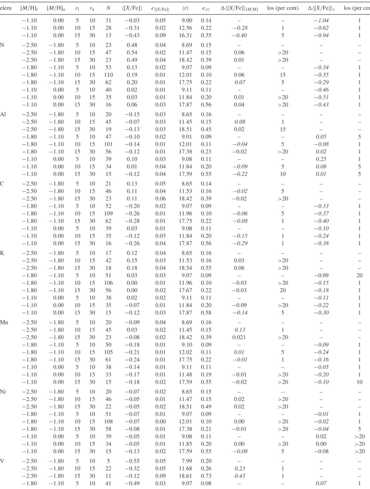
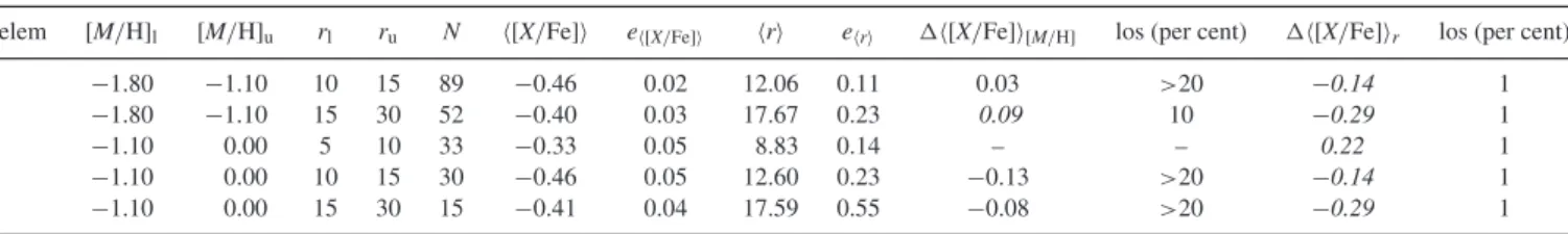
In order to quantify the variation, Table1shows the difference between each median [X/Fe] ratio with the nearest stars median [X/Fe],r<10 kpc, for each range of [M/H] considered and with the lowest metallicity median, −2.5< [M/H]< −1.8, for each range ofr. When the difference is significant [as demonstrated by application of a Kolmogorov–Smirnov (K-S) test – see Section 4.4], it is indicated in italics.

Finally, we verify whether the resulting trends are consistent when taking into account the three sets of available distance es-timates. For this purpose, we analyse whether the variance of the median [X/Fe] ratios, calculated from the distance estimates by the several groups described in Section 4.4, follows the same trends inferred from an individual set of estimates.

4 R E S U LT S

4.1 [X/H] versusr

We evaluate the median [Fe/H] values, as a function ofr, using distances calculated by BPG, H15, and S14. All produce fairly

similar results, but we choose to employ the BPG estimates derived from the peak of the second PDF in their analysis (BPG2p – see Santiago et al.2016). The reason is that it has the least amount of scatter in the [M/H] versusrrelation, and showed little signs of a gradient, which is in agreement with that observed byFA15.

Considering the [M/H] values externally calibrated with [Fe/H] abundances from the literature, the resulting median values (bottom panel in Fig.1) are around∼−1.5, which is consistent with the previous works. As mentioned above in Section 3.1, we have derived the MDF for our sample from the calibrated [M/H], shown in the top panel of Fig.1. The peak of the distribution is around [M/H]

∼ −1.5. In addition, a second peak around−2.1 is observed. This is very close to the median metallicity value associated with the outer-halo region (Carollo et al.2010; Allende Prieto et al.2014; FA15).

The trend of the median [X/H] ratios with distance from the Galactic Centre, shown in Fig.2, exhibits constant or decreasing trends. Those inferred for theα-elements are fairly constant, except [Mg/H] and [Ti/H], which show a significant decrease,∼0.1 dex, fromr<10 tor>15 kpc. [C/H] also exhibits a significant variation, the largest among all the elements evaluated, decreasing by∼0.2 dex fromr<10 to 10<r<15 kpc.

It is important to recall, however, that the abundances of [C/H] and [N/H] can be altered due to mixing events in cool red giants, the dominant spectral class of our sample. Thus, these elements are not reliable indicators of the ISM chemistry from which these stars formed. Although we provide their resulting median values and trends, we will not comment on them because we are interested in those abundances which provide information of the previous stellar populations.

The [Mn/H] abundance exhibits a decreasing trend, contrary to the other iron-peak [Ni/H], which does not show significant variation. The elements [Na/H] and [Al/H] both exhibit decreas-ing trends, although [Na/H] has a larger variance with distance (∼0.4 dex). [Al/H] decreases∼0.1 dex fromr<10 kpc to 10<

r < 15 kpc. Both elements are produced by massive stars and LIMS; however, the production and ejection efficiencies for each element are different. Finally, the [K/H] and [V/H] both show con-stant trends.

We also evaluate [X/H] trends withr, splitting the sample into bins of [M/H]. As expected, [X/H] is higher as [M/H] increases. Overall, the elemental abundances exhibit similar variations withr

and [M/H]. The most metal-rich stars exhibit the largest variation withr, with higher median values for stars in the inner-halo region compared to those in outer-halo region, excepting [Si/H] and [Ti/H] among theα-elements, and [N/H], [Ni/H], and [V/H], which remain constant.

4.2 [X/Fe] versusr

Inspection of the variation of [X/Fe] withrreveals that the chemical trends depend on the metallicity range considered, as seen in Fig.3. For theα-elements, metal-poor stars have enhanced [X/Fe] across allr. The median ratios decrease as the metallicity increases. The most metal-rich stars show the largest variation withr, decreasing farther from the Galactic Centre. This decreasing trend tends to flatten towards lower [M/H], although [Ca/Fe] shows a significant fluctuation of 0.07 dex withrat−2.5<[M/H]<−1.8. [Ti/Fe] decreases 0.14 dex in this metallicity bin.

Figure 3. [X/Fe] median values as a function ofr. The trends are inferred by splitting the sample into the three [M/H] bins shown in the legend of the lower-right panel in the top set of plots.

outer regions. As was found by FA15, [Ca/Fe] exhibits a larger dependence with metallicity than [Mg/Fe]. The decreasing trends of [Ca/Fe] withrin each of the metallicity bins analysed are consistent with theFA15results, although with an offset in the median values. In contrast, the increasing trends observed inFA15for [Mg/Fe] at

[M/H]>−1.1 are not confirmed in this work, where we find that the median ratio decreases.

Figure 4. [X/Fe] median values as a function of [M/H], splitting the sample into threerbins:r<10 kpc, 10<r<15 kpc, andr>15 kpc. to decrease (∼0.08 dex) with distance for stars in the most

metal-rich bin. This pattern is the same observed for theα-elements, in agreement with previous findings (Nissen & Schuster2010,2011; Yamada et al.2013; Hawkins et al.2015), although they detected the pattern from the analysis of [X/Fe] as a function of metallicity.

Table 1. Median [X/Fe] andrwith their corresponding MAD, evaluated in the three [M/H] andrbins, and the difference between each median and that corresponding to the lowestrbin over each [M/H] range and to the lowest [M/H] bin over eachrrange. The significant differences indicated by the K-S test are in italics, followed by the level of significance (los).

elem [M/H]l [M/H]u rl ru N [X/Fe] e[X/Fe] r er [X/Fe][M/H] los (per cent) [X/Fe]r los (per cent)

O −2.50 −1.80 5 10 21 0.40 0.02 8.65 0.15 – – – –

−2.50 −1.80 10 15 47 0.41 0.01 11.46 0.14 0.01 1 – –

−2.50 −1.80 15 30 22 0.35 0.02 18.51 0.42 −0.05 5 – –

−1.80 −1.10 5 10 52 0.30 0.01 9.07 0.09 – – −0.10 1

−1.80 −1.10 10 15 108 0.28 0.00 12.01 0.10 −0.02 15 −0.13 1

−1.80 −1.10 15 30 60 0.26 0.01 17.67 0.22 −0.04 1 −0.09 1

−1.10 0.00 5 10 39 0.26 0.01 9.08 0.11 – – −0.14 1

−1.10 0.00 10 15 34 0.25 0.01 11.85 0.20 −0.01 5 −0.16 1

−1.10 0.00 15 30 16 0.12 0.01 17.87 0.56 −0.14 1 −0.23 1

Mg −2.50 −1.80 5 10 21 0.14 0.03 8.65 0.15 – – – –

−2.50 −1.80 10 15 46 0.24 0.02 11.47 0.15 0.1 15 – –

−2.50 −1.80 15 30 22 0.15 0.03 18.51 0.49 0.01 >20 – –

−1.80 −1.10 5 10 50 0.12 0.01 9.01 0.09 – – −0.02 >20

−1.80 −1.10 10 15 108 0.09 0.01 11.96 0.10 −0.03 10 −0.16 1

−1.80 −1.10 15 30 59 0.06 0.01 17.38 0.20 −0.06 1 −0.08 1

−1.10 0.00 5 10 39 0.18 0.01 9.08 0.11 – – 0.04 1

−1.10 0.00 10 15 34 0.08 0.02 11.85 0.20 −0.1 20 −0.16 1

−1.10 0.00 15 30 16 −0.02 0.02 17.87 0.56 −0.20 1 −0.16 1

Ca −2.50 −1.80 5 10 21 0.27 0.03 8.65 0.15 – – – –

−2.50 −1.80 10 15 46 0.20 0.03 11.47 0.15 −0.07 1 – –

−2.50 −1.80 15 30 22 0.28 0.03 18.51 0.42 −0.01 >20 – –

−1.80 −1.10 5 10 50 0.16 0.01 9.07 0.09 – – −0.11 1

−1.80 −1.10 10 15 105 0.15 0.01 11.96 0.10 −0.01 >20 −0.05 1

−1.80 −1.10 15 30 58 0.11 0.01 17.67 0.22 −0.05 5 −0.16 1

−1.10 0.00 5 10 39 0.12 0.01 9.08 0.11 – – −0.15 1

−1.10 0.00 10 15 35 0.08 0.01 11.84 0.20 −0.04 >20 −0.12 1

−1.10 0.00 15 30 16 0.03 0.01 17.87 0.56 −0.08 1 −0.24 1

S −2.50 −1.80 5 10 22 0.57 0.02 8.69 0.15 – – – –

−2.50 −1.80 10 15 46 0.53 0.02 11.53 0.16 −0.04 10 – –

−2.50 −1.80 15 30 22 0.57 0.03 18.51 0.42 0.00 >20 – –

−1.80 −1.10 5 10 51 0.44 0.01 9.07 0.09 – – −0.13 1

−1.80 −1.10 10 15 107 0.40 0.01 12.01 0.10 −0.04 >20 −0.14 1

−1.80 −1.10 15 30 62 0.36 0.01 17.75 0.22 −0.08 1 −0.21 1

−1.10 0.00 5 10 39 0.36 0.01 9.08 0.11 – – −0.21 1

−1.10 0.00 10 15 35 0.33 0.01 11.84 0.20 −0.03 15 −0.21 1

−1.10 0.00 15 30 16 0.19 0.02 17.87 0.56 −0.17 5 −0.38 1

Si −2.50 −1.80 5 10 22 0.35 0.01 8.69 0.15 – – – –

−2.50 −1.80 10 15 47 0.37 0.01 11.47 0.15 0.02 >20 – –

−2.50 −1.80 15 30 23 0.30 0.01 18.42 0.39 −0.05 10 – –

−1.80 −1.10 5 10 52 0.34 0.01 9.07 0.09 – – 0.00 >20

−1.80 −1.10 10 15 109 0.32 0.00 11.96 0.10 −0.02 >20 −0.05 1

−1.80 −1.10 15 30 62 0.30 0.01 17.75 0.22 −0.04 1 0.00 >20

−1.10 0.00 5 10 39 0.29 0.01 9.08 0.11 – – −0.06 1

−1.10 0.00 10 15 35 0.26 0.01 11.84 0.20 −0.03 >20 −0.11 1

−1.10 0.00 15 30 16 0.22 0.02 17.87 0.56 −0.07 10 −0.08 5

Ti −2.50 −1.80 5 10 18 0.10 0.04 8.65 0.16 – – – –

−2.50 −1.80 10 15 41 0.03 0.02 11.37 0.15 −0.07 >20 – –

−2.50 −1.80 15 30 21 −0.06 0.03 18.42 0.49 −0.14 10 – –

−1.80 −1.10 5 10 49 −0.02 0.01 9.07 0.09 – – −0.12 1

−1.80 −1.10 10 15 105 −0.07 0.01 11.96 0.10 −0.05 1 −0.09 1

−1.80 −1.10 15 30 60 −0.10 0.01 17.67 0.22 −0.08 1 −0.04 1

−1.10 0.00 5 10 39 −0.04 0.02 9.08 0.11 – – −0.14 5

−1.10 0.00 10 15 34 −0.05 0.01 11.85 0.20 −0.01 5 −0.07 1

−1.10 0.00 15 30 15 −0.12 0.02 17.59 0.55 −0.08 5 −0.06 1

Na −2.50 −1.80 5 10 14 1.01 0.08 8.69 0.19 – – – –

−2.50 −1.80 10 15 38 0.32 0.12 11.53 0.18 −0.69 1 – –

−2.50 −1.80 15 30 13 0.52 0.11 18.51 0.38 −0.49 5 – –

−1.80 −1.10 5 10 45 −0.07 0.07 9.01 0.11 – – −1.08 1

−1.80 −1.10 10 15 89 −0.06 0.05 12.01 0.11 −0.01 >20 −0.37 1

Table 1 –continued

elem [M/H]l [M/H]u rl ru N [X/Fe] e[X/Fe] r er [X/Fe][M/H] los (per cent) [X/Fe]r los (per cent)

−1.10 0.00 5 10 31 −0.03 0.05 9.00 0.14 – – −1.04 1

−1.10 0.00 10 15 28 −0.31 0.02 12.56 0.22 −0.28 1 −0.62 1

−1.10 0.00 15 30 13 −0.43 0.09 16.31 0.35 −0.40 5 −0.94 1

N −2.50 −1.80 5 10 23 0.48 0.04 8.69 0.15 – – – –

−2.50 −1.80 10 15 47 0.54 0.02 11.47 0.15 0.06 >20 – –

−2.50 −1.80 15 30 23 0.49 0.04 18.42 0.39 0.01 >20 – –

−1.80 −1.10 5 10 53 0.13 0.02 9.07 0.09 – – −0.34 1

−1.80 −1.10 10 15 110 0.19 0.01 12.01 0.10 0.06 15 −0.35 1

−1.80 −1.10 15 30 62 0.20 0.01 17.75 0.22 0.07 5 −0.29 1

−1.10 0.00 5 10 40 0.02 0.01 9.11 0.11 – – −0.46 1

−1.10 0.00 10 15 35 0.03 0.01 11.84 0.20 0.01 >20 −0.51 1

−1.10 0.00 15 30 16 0.06 0.03 17.87 0.56 0.04 >20 −0.43 1

Al −2.50 −1.80 5 10 20 −0.15 0.03 8.65 0.16 – – – –

−2.50 −1.80 10 15 45 −0.07 0.03 11.45 0.15 0.08 1 – –

−2.50 −1.80 15 30 19 −0.13 0.03 18.51 0.45 0.02 15 – –

−1.80 −1.10 5 10 47 −0.10 0.02 9.01 0.09 – – 0.05 5

−1.80 −1.10 10 15 101 −0.14 0.01 12.01 0.11 −0.04 5 −0.08 1

−1.80 −1.10 15 30 56 −0.12 0.01 17.38 0.23 −0.02 >20 0.02 1

−1.10 0.00 5 10 39 0.10 0.03 9.08 0.11 – – 0.25 1

−1.10 0.00 10 15 34 0.01 0.04 11.84 0.20 −0.09 5 0.08 5

−1.10 0.00 15 30 15 −0.12 0.04 17.59 0.55 −0.22 10 0.01 5

C −2.50 −1.80 5 10 21 0.13 0.05 8.65 0.14 – – – –

−2.50 −1.80 10 15 46 0.11 0.04 11.53 0.16 −0.02 5 – –

−2.50 −1.80 15 30 23 0.11 0.06 18.42 0.39 −0.02 >20 – –

−1.80 −1.10 5 10 52 −0.20 0.02 9.07 0.09 – – −0.33 1

−1.80 −1.10 10 15 109 −0.26 0.01 11.96 0.10 −0.06 5 −0.37 1

−1.80 −1.10 15 30 62 −0.28 0.01 17.75 0.22 −0.08 1 −0.40 1

−1.10 0.00 5 10 39 0.03 0.01 9.08 0.11 – – −0.10 1

−1.10 0.00 10 15 35 −0.12 0.03 11.84 0.20 −0.15 1 −0.24 1

−1.10 0.00 15 30 16 −0.26 0.04 17.87 0.56 −0.29 1 −0.38 1

K −2.50 −1.80 5 10 17 0.12 0.04 8.65 0.16 – – – –

−2.50 −1.80 10 15 42 0.15 0.03 11.53 0.16 0.03 >20 – –

−2.50 −1.80 15 30 18 0.18 0.04 18.54 0.55 0.06 >20 – –

−1.80 −1.10 5 10 51 0.03 0.03 9.07 0.09 – – −0.09 20

−1.80 −1.10 10 15 106 0.00 0.01 11.96 0.10 −0.03 >20 −0.15 1

−1.80 −1.10 15 30 56 0.00 0.02 17.67 0.22 −0.03 20 −0.18 1

−1.10 0.00 5 10 38 0.02 0.02 9.11 0.11 – – −0.11 1

−1.10 0.00 10 15 35 −0.07 0.01 11.84 0.20 −0.09 >20 −0.22 1

−1.10 0.00 15 30 15 −0.12 0.03 17.87 0.58 −0.14 5 −0.30 1

Mn −2.50 −1.80 5 10 20 −0.09 0.04 8.69 0.16 – – – –

−2.50 −1.80 10 15 45 0.03 0.02 11.45 0.15 0.13 1 – –

−2.50 −1.80 15 30 23 −0.08 0.02 18.42 0.39 0.021 >20 – –

−1.80 −1.10 5 10 50 −0.18 0.01 9.10 0.09 – – −0.09 1

−1.80 −1.10 10 15 105 −0.21 0.01 12.02 0.11 0.01 5 −0.24 1

−1.80 −1.10 15 30 61 −0.24 0.01 17.75 0.22 −0.01 1 −0.16 1

−1.10 0.00 5 10 38 −0.14 0.01 9.11 0.11 – – −0.05 1

−1.10 0.00 10 15 33 −0.17 0.01 11.48 0.19 −0.01 >20 −0.20 1

−1.10 0.00 15 30 15 −0.18 0.02 17.59 0.55 −0.02 >20 −0.10 10

Ni −2.50 −1.80 5 10 20 −0.07 0.02 8.65 0.15 – – – –

−2.50 −1.80 10 15 46 −0.05 0.01 11.47 0.15 0.02 >20 – –

−2.50 −1.80 15 30 22 −0.05 0.02 18.51 0.49 0.02 >20 – –

−1.80 −1.10 5 10 51 −0.07 0.01 9.07 0.09 – – −0.01 1

−1.80 −1.10 10 15 108 −0.07 0.00 12.01 0.10 0.00 >20 −0.02 1

−1.80 −1.10 15 30 58 −0.08 0.01 17.38 0.21 −0.01 >20 −0.04 5

−1.10 0.00 5 10 39 −0.05 0.01 9.08 0.11 – – 0.02 >20

−1.10 0.00 10 15 34 −0.05 0.01 11.85 0.20 0.00 >20 0.00 >20

−1.10 0.00 15 30 15 −0.13 0.02 17.59 0.55 −0.08 5 −0.08 >20

V −2.50 −1.80 5 10 5 −0.55 0.05 7.99 0.20 – – – –

−2.50 −1.80 10 15 22 −0.32 0.05 11.68 0.26 0.23 1 – –

−2.50 −1.80 15 30 11 −0.12 0.09 18.61 0.73 0.43 1 – –

Table 1 –continued

as metallicity increases. This ratio decreases with rfor the most metal-rich stars, while it tends to increase for the most metal-poor stars. As a consequence, stars in the outer region have [Al/Fe] which does not depend so significantly on metallicity than for stars in the inner region. The theoretical Na and Al yields predict similar [X/Fe] versus [Fe/H] behaviours. However, observations in the solar neighbourhood do not completely follow the theoretical predictions (Cˆot´e et al. 2016). Our analysis also reveals a disagreement in [Na/Fe] and [Al/Fe] trends withrand [M/H].

The ratio [K/Fe] also tends to decrease withrat [M/H]∼−1.1, but stars at [M/H]<−1.1 exhibit constant trends. The difference in [K/Fe] with [M/H] is higher for stars in the outer region. [V/Fe] increases withrin the most metal-poor stars, and tends to flatten as [M/H] increases, although no well-defined trends with metal-licity are observed. The chemical analysis of V should be taken with caution, however, because its measurement is less reliable (V is determined exclusively from very weak spectral features – see Holtzman et al.2015).

4.3 [X/Fe] versus [M/H]

The resulting curves of the median [X/Fe] values, calculated as a function of [M/H], are shown in Fig.4. Overall,α-elements show decreasing trends with [M/H], with few exceptions. Stars atr <

10 kpc exhibit a decrease larger than 0.1 dex in [X/Fe] towards higher [M/H], except for [Mg/Fe] and [Si/Fe]. These abundances remain constant and slightly vary at [M/H]∼1.1, increasing 0.04 dex and decreasing 0.06 dex, respectively.

Asrincreases, the trends become steeper (except for [Ti/Fe], which tends to flatten). The most distant stars show decreasing vari-ations>0.1 dex for [Mg/Fe],>0.2 dex for [O/Fe] and [Ca/Fe], and

>0.3 dex for [S/Fe]. [Si/Fe] and [Ti/Fe] also decrease with [M/H], although less (<0.1 dex). Fig.4clearly shows the spread in [α/M] for stars at [M/H]>−1.1 as a function of distance from the Galactic Centre described in the previous section. This spread,≥0.1 dex, is similar to the differences observed by Nissen & Schuster (2010) for [α/Fe] as a function of [Fe/H].

Based on the K-S test, no significant variations larger than 0.1 dex are detected in [Ni/Fe] with [M/H]. However, Fig.2reveals lower [Ni/Fe] asrincreases at [M/H]∼ −1.1. The [Mn/Fe] ratio decreases with [M/H] from the most metal-poor stars up to [M/H]∼ −1.5, and increases slightly towards higher metallicities. The increasing trend on the higher metallicity side is independent of distance; all the stars in the sample have similar median [Mn/Fe] ratios. In contrast, the metal-poor tail suggests enhanced [Mn/Fe] ratios for more distant stars.

There is an overall decrease of [Na/Fe] with [M/H]. The [Na/Fe] ratio exhibits the largest variation, but also a large scatter, likely due to the difficulty of measuring Na from the APOGEE spectra (Holtzman et al.2015). The variation of [Al/Fe] with [M/H] clearly depends on the distance bin considered. The nearest stars exhibit an increasing trend, with variations of∼0.25 dex between stars with

[M/H]<−1.8 and [M/H]>−1.1. This trend tends to flatten withr. The [Al/Fe] ratio for stars atr>15 kpc is nearly constant. Thus, for [M/H]>−1.1, the median [Al/Fe] decreases withr. The metal-poor stars suggest an opposite trend withr.

The median [K/Fe] ratios also reflect a different enrichment pat-tern which depends on Galactocentric distance. Trends are steeper asrincreases, with enhanced ratios in the metal-poor tail and lower values towards the highest metallicities which we consider. At [M/H] −1.5, there is no significant difference in the median ratios calculated for the three distance bins.

We find an increasing trend in [V/Fe] with distance for stars at

r<10 kpc, flattening asrincreases. Our resulting ratios have lower median [V/Fe] ratios for all the stars in our sample. Overall, distant stars have higher [V/Fe], and the trends for the threerbins merge for stars with [M/H]>−1.1. However, as mentioned above, estimates of the V abundance are less reliable due to its weak features in APOGEE spectra.

4.4 Validation of trends

In order to check whether the resulting trends reported above de-pend on the chosen distance estimates, we calculate the median abundance ratios for the six sets of distances available for DR12 APOGEE data. We first calculate the median and its variance for each of the six median abundance ratios in the correspondingrand [Fe/H] bins, and then evaluate how these variances change with

rand [M/H]. Overall, these curves confirm the previous inferred trends. Thus, the different distance estimates lead to the same qual-itative trends, although the particular median values differ slightly depending on the set of distances considered.

As an additional check, we carried out the previous evaluations by considering the mean ratios weighted with the measurement errors – the resulting trends are qualitatively similar to the median ratio curves. We also performed a K-S test in order to verify if the observed differences between our median ratios over bins inrand [M/H] are statistically significant. We proceed by calculating the cumulative distribution function (CDF) for each bin inrand [M/H] evaluated, and the maximum difference between each CDF and the CDF corresponding to the lowestrbin over each [M/H] range (and to the lowest [M/H] bin over eachrrange), then compare with the critical values of the K-S statistic. In order to consider a difference significant, we demand that it cannot be rejected at higher than the 10 per cent level. We perform the test to evaluate variations of [X/H] versusr and [X/Fe] versusr and [M/H]. The last four columns in Table1show the resulting variations in [X/Fe] as a function ofrand [M/H] and the level of significance obtained for them; those with a significant difference are indicated in italics. In the previous sections, we have only described significant variations after applying this test.

[X/H] is affected by the same systematic deviation. If this is the case, the deviation would be absent in the resulting [X/Fe]. In contrast, the ratios would be systematically underestimated towards lower metallicities. In most of the cases, the observed [X/Fe] trends with metallicity are the opposite. The slopes would be higher if [X/Fe] were underestimated.

Uncertainties in the stellar parameters could lead to systematic errors in the chemical abundances and thus distortions in the in-ferred chemical trends. M´esz´aros et al. (2015) investigated about the deviations in [Fe/H], [C/Fe], [N/Fe], and [_α/Fe] (each of the ASPCAPα-elements) due to uncertainties inTeff. From their fig. 3, we observe that the most sensible ratio to aTeffvariation is [O/Fe]. ATeff∼200 K would imply alogg∼0.6 dex in the red giant branch (RGB), and an uncertainty in [O/Fe]∼0.25 dex (lower for the other abundances of our interest). The peak of the logg distribu-tion in ther<10 andr>15 kpc bins shifts towards 0.5 dex lower, approximately. Considering the number of the stars in our furthest bin, we derive that the possible systematic error due to uncertainties in the parameters would lead to underestimate 0.08 dex our [O/Fe]. However, we detect a larger variation at the most metal-rich side.

The APOGEE sample comprises stars in the RGB and possibly in the asymptotic giant branch (AGB) stages of evolution. These stages are reached by LIMS, producing, at the same time, heavy elements with diverse efficiencies, depending on the initial mass and metallicity of the stars. The photospheres of these stars are enriched mainly by carbon, nitrogen, fluorine, and heavier elements synthesized by the slow neutron capture process (thes-process) and by proton-capture nucleosynthesis (thep-process). The mixing from the interior (core and shells surrounding the core) to the stellar envelope results in self-pollution of the stellar photosphere.

The abundances of all theα-elements analysed in this paper (O, Mg, Si, S, Ca, Ti) are representative of those abundances in the ISM from which the stars formed, because these chemical elements are not synthesized and are not carried to the photosphere of LIMS (see review by Karakas & Lattanzio2014). Moreover, half of the other elements studied in this work (K, V, Mn, Ni) are also not generated by LIMS. Therefore, our results for O, Mg, Si, S, Ca, Ti, K, V, Mn, Ni are independent of the evolutionary status of the APOGEE stars. Nevertheless, C, N, Na, and Al are produced by LIMS, but in very different proportions. Among these four elements:

(i) C is the most produced, mainly by low-mass stars (M <

3.5 M) during the thermal pulses and the third dredge-up (dur-ing the AGB);

(ii) N is the second most produced, mainly by intermediate-mass stars (M>3.5 M) during the first and second dredge-ups (during the ascent of the RGB and AGB, respectively) and hot bottom burning;

(iii) Na and Al are synthesized mainly by stars withM>3.5 M during the second and third dredge-ups, with Na more abundantly produced than Al.

Since C and N are mainly produced by LIMS, we caution that C and N do not reliably represent the original stellar abundances. The Na and Al abundances might be enhanced at high Galactocentric radii, because

(i) these elements are produced by intermediate-mass stars in evolved stages (AGB) and consequently by more luminous stars, and

(ii) the APOGEE sample at largermay be more weighted to-wards these more luminous objects.

However, ther-trends of Na and Al (Figs2and3) appear to show no enhancement at large radii.

Stars at different distances could also have different age distribu-tions: at the bottom of the giant branch stars may be biased towards a different age distribution than at the upper side, which might affect the overall chemical trends. Nearer stars would be biased towards slightly younger and more metal-rich stars and further stars towards older and more metal-poor ones; however, if it were the case, further stars would show higher [α/Fe] ratios, because older stars would have formed from an ISM mainly enriched by SNeII. Our analysis reveals the opposite trend with galactocentric distance.

Finally, we estimate the impact of the distance errors in our sample. We assume a normal distribution with uncertainties of 20 per cent, and add this noise to the BPG distance values. The resulting fraction of stars with |zn| >5 (after adding the noise) but|z| <5 (without noise), with respect to the stars with |z|>

5, is 40 per cent forr<10 kpc, 13 per cent for 10<r<15 kpc, and 3 per cent forr>15 kpc. However, these fractions reduce to 1 per cent and lower if we consider stars at|zn|<4. This means that there could be a contamination of ∼40 per cent of stars at 4< |z|< 5 kpc in our r< 10 bin. At this|z|range, the den-sity of thin disc stars is negligible, of thick disc stars is∼2 per cent the density of stars in the plane, and a little less for the density of halo stars. Thus, 50–70 per cent of the contaminant stars, i.e. a∼20– 30 per cent of the stars in ther<10 kpc bin, are likely to belong to the thick disc. The resultant median abundances would be domi-nated by halo stars. Besides, previous works have not found differ-ences in chemistry between thick disc and halo stars. Therefore, we assert that the chemical trends would not be greatly distorted by this contamination.

5 D I S C U S S I O N

Differences for a number of the chemical trends with [M/H] are clear between stars atr_<10 andr_>15 kpc. The lower_α -element-to-iron ratios found at larger distances are consistent with the low-α

population reported during the past decade by a number of work-ers (e.g. Fulbright 2002; Gratton et al.2003; Nissen & Schus-ter 2010, 2011; Ishigaki, Chiba & Aoki2012; Ishigaki, Aoki & Chiba2013; Hawkins et al.2015). From the kinematical properties of their samples, they estimated that the orbits of these stars would place them farther away than stars exhibiting higher [α/Fe] ratios. This is consistent with our finding (and that ofFA15).

Our present study finds a decrease withr consistent with that obtained byFA15atr<20 kpc. They also observed a considerably larger drop occurring at a Galactocentric radius between 20<r<

40 kpc, which we cannot confirm in this work, as the APOGEE observations do not extend to cover this distance range.

The trend observed with [M/H] for the low-[α/Fe] population has been interpreted in terms of SNeIa, which contribute iron but littleα-elements. The differences in [X/Fe] observed in the present work between stars at r < 10 kpc and r > 15 kpc for the α -elements (∼0.1 dex for Si, Ca, and Ti, and higher for O, Mg, and S) are consistent with their expected relative contributions in SNeIa explosions (Tsujimoto et al.1995) – higher for Si (17 per cent) and Ca (25 per cent) than for Mg, O, and S (negligible).

high-_αstars would form during the early bursts, while the low-_α stars would form at the beginning of later bursts from an ISM con-taminated by recent SNeIa, as appears to have occurred in dwarf spheroidal galaxies (see, e.g., Carigi, Hernandez & Gilmore2002). Nissen & Schuster (2010) also proposed that the low-α popula-tion could be born in systems which were later accreted into the Milky Way’s halo, and which had experienced a long star formation history.

However, the decrease in [α/Fe] ratios due to the contribution of SNeIa encounters difficulty in explaining the pattern of some abun-dance ratios, in particular, the decrease observed for [Ni/Fe] with metallicity for the low-αpopulation, and the absence of different [Mn/Fe] ratios between both populations. These two elements are expected to be released by SNeIa; thus, different patterns should be detected in Ni and Mn with respect to iron between stars formed in an ISM enriched by SNeIa and stars which formed from gas without their contribution. In fact, it would be expected that low-α

stars would have higher [Ni/Fe] and [Mn/Fe] than the high-αstars. However, this is not seen either in our work or in previous studies.

A possible explanation was suggested by Kobayashi et al. (2006), who claimed that, for an IMF biased towards stars which explode as low-mass SNIe-II, this would lead to lower [α/Fe]. Kobayashi et al. (2014) also proposed that the nucleosynthesis of 10–20 Mstars could explain the difference in the [α/Fe] ratios detected in halo stars. Interestingly, McWilliam, Wallerstein & Mottini (2013) also claimed that a ‘top-light’ IMF might provide an explanation for the [α/Fe] and [Eu/Fe] deficiencies found in the analysis of the M54 cluster belonging to the Sagittarius dwarf spheroidal galaxy. This possibility would also explain the [Mn/Fe] and [Ni/Fe] patterns, but it would imply a complex IMF behaviour to explain the different trends – a metallicity-dependent IMF for the low-α stars and a metallicity-independent IMF for the high-αpopulation, as Nissen & Schuster (2011) indicated.

Another remaining issue is the fact that the nucleosynthetic con-tribution from AGB stars (the immediate progenitors of the white dwarfs involved in SNeIa explosions) should be detected in the low-αpopulation, if SNeIa have contributed their iron. However, these stars exhibitlower[Na/Fe] ratios than the stars presumed to be formed prior to the contributions from SNeIa. As Nissen et al. (2014) speculated, this could be the result if the progenitors of the low-αpopulation were stars of intermediate mass (4–8 M), which contribute little C to the ISM, and even less Na and Al. The lower median [Na/Fe] and [Al/Fe] ratios which we found for stars atr

>15 kpc are consistent with a slow chemical-enrichment history. No signature of significant enrichment from AGBs (neither Na nor Al) is detected in the distance bin where the low-αpopulation dom-inates.

The observed increase in [Al/Fe] observed for stars in the in-ner regions can be explained with the assumption of metallicity-dependent yields for massive stars (Nomoto, Kobayashi & Tomi-naga2013), and the flat trend with [M/H] for the farthest stars by the cancellation of the increase in Al by the even higher contribu-tion of Fe from SNeIa. However, we do not detect an increasing trend of [Na/Fe] with [M/H] in the nearest stars, as observed by Nissen & Schuster (2010) for the high-αpopulation, which is well explained by the same metallicity-dependent yields also invoked for Na (Nomoto et al.2013). Observationally, Na is determined by APOGEE from relatively weak lines in theHband, yielding less accurate measurements, as suggested by the large scatter detected in our sample as well as in Holtzman et al. (2015), when inspecting [Na/Fe] versus [Fe/H]. For these reasons, our Na results should be considered with caution.

The higher [X/Fe] ratios at metallicities lower than−1.8 but lower ratios at higher metallicities may be explained by the com-bination of a top-heavy IMF and a slower SFR in the subsystems accreted by the Galaxy. Recent cosmological simulations predict that massive satellites merging with the host galaxy contribute at smaller radii than low-mass systems (Amorisco2015). Low-mass systems are expected to experience outflows which release their gas. This would prevent, or at least greatly suppress, subsequent star formation. The expected IMF for low-mass stellar systems at low metallicities is characterized by discontinuities, i.e. a lack of some massive stars (Cervi˜no2013). The signature of the few high-mass stars in such low-metallicity environments produces stochastic effects on the abundance ratios (Carigi & Hern´andez2008), which could explain the higher dispersion observed in [X/Fe] for metal-poor stars.

The stars which we observe today at metallicities lower than

−1.8, born in these low-mass subsystems, would be formed from the nucleosynthetic contribution from a few very massive stars, leading to high ratios with respect to iron at very low metallicities, followed by less massive stars slowly contributing to the ISM where the current stars were born. In contrast, the inner regions would be formed in an ISM which would have reached the same metallicity faster, with the contribution of a larger number of massive stars, although the upper mass limit of the IMF would be lower (Yamada et al.2013).

6 C O N C L U S I O N S

We have analysed a sample of ∼400 halo stars targeted by the APOGEE survey, located at|z|>5 kpc from the Galactic plane, and evaluated the chemical trends for the 15 individual abundances determined by ASPCAP. In order to be sure that our trends were not unduly influenced by the estimated distances to our stars, we made use of the available distances estimated by three independent meth-ods for APOGEE stars. Our main conclusions are the following.

(i) An analysis of the elemental abundance ([X/H]) variation with distance from the Galactic Centre,r, up to the farthest distances observed by APOGEE (∼20–30 kpc), revealed that the chemical trends are almost constant or decrease withr. The variation mainly occurred for stars with a global metallicity [M/H]>−1.1.

(ii) We confirmed that the qualitative chemical trends inferred from our data do not depend on the considered distance set.

(iii) The resulting iron abundance trend calculated from the cali-brated [M/H] parameter is constant across the range ofrexamined, 5 r 30 kpc. The variation for nearer stars measured in our analysis is barely lower than that observed in the previous analysis ofin situhalo stars performed byFA15with SDSS optical spectra at lower resolution. They also reported a larger decrease taking place at 20_<r_<40 kpc. Our evaluation of [Fe/H] and [Ca/H] is consis-tent with their results, but we cannot probe the chemical trends at 20<r<40 kpc due to a lack of sample stars in this distance range. (iv) The median calibrated [M/H] values,∼−1.5, also agree with previous reports for inner-halo stars (Carollo et al. 2007, 2010; Chen et al. 2014; FA15). The derived MDF from [M/H] also shows a second peak at [M/H]∼ −2.1, which resembles the me-dian metallicity value associated with the outer-halo population (Carollo et al.2007,2010; Beers et al.2012).

population of stars with different_α-element enrichment becomes dominant beyondr∼15 kpc.

(a) For the α-elements, we found significantly lower ratios for more distant stars at metallicities [M/H]>−1.1. We observed a larger separation in these two populations for [O/Fe], [Mg/Fe], and [S/Fe], but all the α-elements show a significant decrease of0.1 dex.

Our [Ca/Fe] results withrand [M/H] are consistent with the results reported byFA15based on SDSS optical spectra. In contrast, we found a decreasing trend of [Mg/Fe] with distance, which disagrees with what they observed.

Our results are also consistent with the two different halo popu-lations reported in APOGEE data by Hawkins et al. (2015) at−1.2

<[M/H]<−0.55. The [O/Fe] and [Mg/Fe] trends we observed are in agreement with their work and other previous reports. Con-versely, we found that the two populations also exhibit different [S/Fe] ratios.

(b) We find hints of low-αstars having lower [Ni/Fe]. We detect different [Mn/Fe] ratios between the inner and outer regions for the most metal-poor stars ([M/H]<−1.8), although a larger sample of stars at distances farther than 15 kpc and more accurate measure-ments are necessary to confirm this result.

(c) The [K/Fe] trends withrand [M/H] also provide evidence for different chemical abundance patterns in stars atr< 10 kpc and

r>15 kpc.

(d) Both [Na/Fe] and [Al/Fe] reveal different chemical patterns for the nearer stars compared with the more distant stars. The [Na/Fe] ratio exhibits different trends with r and [M/H] than found for [Al/Fe], but the Na measurements are less reliable. The [Al/Fe] ratio increases with metallicity for inner-halo stars, while the more distant stars exhibit a flat trend.

This work corroborates the suggestion that stars with low [α/Fe] ratios are predominant at larger distances than stars with higher [α/Fe] ratios, in agreement with previous work which inferred the distances for the low- and high-αpopulations based on their kinematical properties (Ishigaki et al. 2010; Nissen & Schus-ter2010,2011). The lower [α/Fe] ratios are consistent with iron enrichment due to SNeIa; the [Al/Fe] chemical patterns are also consistent with this hypothesis. The [Ni/Fe] and [Mn/Fe] exhibit trends with metallicity in both populations which are also consis-tent with these previous studies. However, their chemical patterns, as well as the lack of signatures of AGB enrichment, are not those expected in a scenario where SNeIa had time to explode. The char-acteristics of the environments where both populations were formed remain unclear.

In conclusion, the chemical trends inferred for stars ranging over distances from the Galactic Centre of 5< r < 30 kpc suggest that, atr>15 kpc, a stellar population begins to dominate which formed with a different chemical-enrichment history than stars at

r< 10 kpc. Characterization of the different stellar populations with a larger sample of stars will better constrain the IMF and SFR associated with these previous stellar populations. High-quality data for stars atrfarther than 15 kpc will help to clarify the chemical properties of the more distant stellar populations in the Galactic halo. Alternatively, the identification of nearby halo stars which probe to large distances (on the basis of their extreme kinematics) will also permit an increase in the number of suitable outer-halo stars for further analysis.

AC K N OW L E D G E M E N T S

EFA acknowledges support from Direcci´on General de Asuntos del Personal Acad´emico (DGAPA)-Universidad Nacional Aut´onoma de M´exido (UNAM) postdoctoral fellowships. LC thanks for the financial supports provided by Consejo Nacional de Ciencia y Tecnolog´ıa (CONACyT) of M´exico (grant 241732), by Programa de Apoyo a Proyectos de Investigaci´on e Innovaci´on Tecnol´ogica (PAPIIT) of M´exico (IG100115, IA100815), and by Ministerio de Econom´ıa, Industria y Competitividad (MINECO) of Spain (AYA2010-16717). TCB acknowledges partial support for this work from grants PHY 08-22648; Physics Frontier Center/Joint Institute for Nuclear Astrophysics (JINA), and PHY-1430152; Physics Fron-tier Center/JINA Center for the Evolution of the Elements (JINA-CEE), awarded by the US National Science Foundation. Funding for SDSS-III has been provided by the Alfred P. Sloan Foundation, the Participating Institutions, the National Science Foundation, and the US Department of Energy Office of Science. The SDSS-III website ishttp://www.sdss3.org/.

SDSS-III is managed by the Astrophysical Research Consor-tium for the Participating Institutions of the SDSS-III Collab-oration including the University of Arizona, the Brazilian Par-ticipation Group, Brookhaven National Laboratory, University of Cambridge, Carnegie Mellon University, University of Florida, the French Participation Group, the German Participation Group, Harvard University, the Instituto de Astrofisica de Canarias, the Michigan State/Notre Dame/JINA Participation Group, Johns Hop-kins University, Lawrence Berkeley National Laboratory, Max Planck Institute for Astrophysics, Max Planck Institute for Ex-traterrestrial Physics, New Mexico State University, New York University, Ohio State University, Pennsylvania State University, University of Portsmouth, Princeton University, the Spanish Par-ticipation Group, University of Tokyo, University of Utah, Vander-bilt University, University of Virginia, University of Washington, and Yale University.

R E F E R E N C E S

Alam S. et al., 2015, ApJS, 219, 12

Allende Prieto C., Beers T. C., Wilhelm R., Newberg H. J., Rockosi C. M., Yanny B., Lee Y. S., 2006, ApJ, 636, 804

Allende Prieto C. et al., 2014, A&A, 568, A7 Amorisco N. C., 2015, MNRAS, 450, 575 An D. et al., 2013, ApJ, 763, 65

An D., Beers T. C., Santucci R. M., Carollo D., Placco V. M., Lee Y. S., Rossi S., 2015, ApJ, 813, L28

Beers T. C. et al., 2012, ApJ, 746, 34 Belokurov V. et al., 2009, MNRAS, 397, 1748 Binney J. et al., 2014, MNRAS, 437, 351 Bovy J. et al., 2014, ApJ, 790, 127

Bressan A., Marigo P., Girardi L., Salasnich B., Dal Cero C., Rubele S., Nanni A., 2012, MNRAS, 427, 127

Burnett B., Binney J., 2010, MNRAS, 407, 339 Burnett B. et al., 2011, A&A, 532, A113 Carigi L., Hern´andez X., 2008, MNRAS, 390, 582

Carigi L., Hernandez X., Gilmore G., 2002, MNRAS, 334, 117 Carollo D. et al., 2007, Nature, 450, 1020

Carollo D. et al., 2010, ApJ, 712, 692 Cervi˜no M., 2013, New Astron. Rev., 57, 123

Chen Y. Q., Zhao G., Carrell K., Zhao J. K., Tan K. F., Nissen P. E., Wei P., 2014, ApJ, 795, 52

Cˆot´e B., Ritter C., O’Shea B. W., Herwig F., Pignatari M., Jones S., Fryer C. L., 2016, ApJ, 824, 82

Eisenstein D. J. et al., 2011, AJ, 142, 72

Fern´andez-Alvar E. et al., 2015, A&A, 577, A81 (FA15)

Fern´andez-Trincado J. G. et al., 2016, ApJ, preprint (arXiv:1604.01279) Fulbright J. P., 2002, AJ, 123, 404

Garc´ıa P´erez A. E. et al., 2016, AJ, 151, 144 Ghez A. M. et al., 2008, ApJ, 689, 1044

Gratton R. G., Carretta E., Desidera S., Lucatello S., Mazzei P., Barbieri M., 2003, A&A, 406, 131

Gunn J. E. et al., 2006, AJ, 131, 2332

Hawkins K., Jofr´e P., Masseron T., Gilmore G., 2015, MNRAS, 453, 758 Hayden M. R. et al., 2015, ApJ, 808, 132 (H15)

Holtzman J. A. et al., 2015, AJ, 150, 148

Ishigaki M., Chiba M., Aoki W., 2010, PASJ, 62, 143 Ishigaki M. N., Chiba M., Aoki W., 2012, ApJ, 753, 64 Ishigaki M. N., Aoki W., Chiba M., 2013, ApJ, 771, 67 Janesh W. et al., 2016, ApJ, 816, 80

Karakas A. I., Lattanzio J. C., 2014, PASA, 31, e030

Kobayashi C., Umeda H., Nomoto K., Tominaga N., Ohkubo T., 2006, ApJ, 653, 1145

Kobayashi C., Ishigaki M. N., Tominaga N., Nomoto K., 2014, ApJ, 785, L5

Lind K. et al., 2015, A&A, 575, L12

McWilliam A., Wallerstein G., Mottini M., 2013, ApJ, 778, 149 Majewski S. R. et al., 2015, AJ, preprint (arXiv:1509.05420)

Marigo P., Girardi L., Bressan A., Groenewegen M. A. T., Silva L., Granato G. L., 2008, A&A, 482, 883

M´esz´aros S. et al., 2015, AJ, 149, 153 Nidever D. L. et al., 2015, AJ, 150, 173

Nissen P. E., Schuster W. J., 2010, A&A, 511, L10 Nissen P. E., Schuster W. J., 2011, A&A, 530, A15

Nissen P. E., Chen Y. Q., Carigi L., Schuster W. J., Zhao G., 2014, A&A, 568, A25

Nomoto K., Kobayashi C., Tominaga N., 2013, ARA&A, 51, 457 Pinsonneault M. H. et al., 2014, ApJS, 215, 19

Santiago B. X. et al., 2016, A&A, 585, A42 Schultheis M. et al., 2014, AJ, 148, 24 (S14)

Tissera P. B., Beers T. C., Carollo D., Scannapieco C., 2014, MNRAS, 439, 3128

Tsujimoto T., Nomoto K., Yoshii Y., Hashimoto M., Yanagida S., Thielemann F.-K., 1995, MNRAS, 277, 945

Yamada S., Suda T., Komiya Y., Aoki W., Fujimoto M. Y., 2013, MNRAS, 436, 1362

Yanny B. et al., 2009, AJ, 137, 4377 York D. G. et al., 2000, AJ, 120, 1579

Zacharias N., Finch C. T., Girard T. M., Henden A., Bartlett J. L., Monet D. G., Zacharias M. I., 2013, AJ, 145, 44

Zasowski G. et al., 2013, AJ, 146, 81