Optimal portfolios in defined contribution pension systems

Texto completo

(1)Revista ABANTE, Vol. 9, Nº 2, pp. 99-129 (octubre 2006). OPTIMAL PORTFOLIOS IN DEFINED CONTRIBUTION PENSION SYSTEMS EDUARDO WALKER* ABSTRACT We study optimal portfolios for defined contribution (possibly mandatory) pension systems, which maximize expected pensions subject to a risk level. By explicitly considering the present value of future individual contributions and changing the risk-return numeraire to future pension units we obtain interesting insights, consistent with the literature, in a simpler context. Results naturally imply that the local indexed (inflation-adjusted) currency is the benchmark and that the investment horizon is long. Optimal portfolios have a hedging component with an even longer duration than a deferred (real) pension, which begins its lifetime payments upon retirement. Results are illustrated with the parameters obtained for the United States by Campbell and Viceira (2001). It also discusses the implications for emerging market reformed pension systems. Keywords: Optimal portfolio, Defined contribution, Pension reform, Deferred pension, Emerging markets JEL: G11, G18, G23 RESUMEN Se estudian los portafolios óptimos para sistemas de pensiones (posiblemente obligatorios) de contribuciones definidas, que maximizan las pensiones esperadas sujetas a un nivel de riesgo. Al considerar el valor presente de las contribuciones futuras a las cuentas individuales y cambiar el numerario de la relación riesgo-retorno a unidades de pensión futura se obtienen intuiciones interesantes, coherentes con la literatura, en un contexto más simple. Los resultados naturalmente implican que la moneda de referencia pertinente es la moneda local indizada a la inflación y que el horizonte es largo. Los portafolios *. Professor, School of Business, Pontificia Universidad Católica de Chile. ewalker@faceapuc.cl; Vicuña Mackenna 4860, Santiago, Chile. I appreciate the comments to previous versions of this work by the participants to the following seminars: “Investment Round Table by Fidelity” (Villarrica, Chile, October 2003); research seminar of Facultad de Ciencias Económicas y Administrativas (Reñaca, Chile, January 2004), particularly Felipe Zurita; Latin America Econometric Society (July 2004). I also thank an anonymous referee and Felipe Varas for very useful comments and suggestions. The opinions herein only represent the author’s..

(2) 100. REVISTA ABANTE, VOL. 9, Nº 2. óptimos tienen un componente de protección con una duración incluso mayor que la de una renta vitalicia diferida, cuyos pagos empiezan a recibirse junto con la jubilación. Los resultados se ilustran con los parámetros obtenidos para Estados Unidos por Campbell y Viceira en (2001). También se discuten las implicancias para los nuevos sistemas de pensiones adoptados en diversos mercados emergentes.. We study optimal portfolios for defined contribution (possibly mandatory) pension systems. Specifically, we consider the perspective of an individual pension account holder who wishes to maximize her expected pension level subject to a certain risk level. We do not consider whether market incentives eventually lead a pension system to provide some kind of optimal portfolio. We also ignore the interrelationship that may exist between current consumption-savings-portfolio decisions and pension fund decisions, which affect consumption upon retirement, assuming that these decisions are made independently. This could be justified in the context of “mental accounting” (Thaler (1985)), or more simply, by considering that in some pension systems people are institutionally forced to save for retirement in a single-purpose individual pension fund account. Naturally, in a Modigliani-Miller spirit, fully rational individuals could partially or completely undo in their own portfolios whatever decision is made in the delegated pension fund portfolio. Therefore, results presented here may be relevant for those who cannot undo these decisions. The question thus is what constitutes an optimal asset allocation from a long-term perspective, considering the available funds in the individual account and a sequence of future contributions to it. As such, this problem has not been solved, at least stated in this way, but closely related problems have been solved before and some of our results turn out to be applications or particular cases. However, from the analysis presented here some interesting and new results arise. A (perhaps novel) way of summarizing the problem is to restate it by changing the numeraire: both expected returns and risk have to be measured in real future pension units. By doing this our analysis naturally emphasizes the issue of reinvestment risk, making it different to maximizing the utility of wealth upon retirement, and this guides our analysis. The benchmark naturally becomes the local inflation-adjusted currency and the horizon becomes long-term. From the perspective of a future pensioner, short-term instruments are not risk free since they have low correlation with the future cost of a pension. For hedging purposes, we are interested in assets whose.

(3) OPTIMAL PORTFOLIO IN DEFINED CONTRIBUTION. 101. returns are highly correlated with variations in future pensioncosts, and these naturally are long-term local indexed bonds, although certain kinds of equity may have good hedging properties too. In any case, taking as reference a deferred (real) pension, which begins lifetime payments upon retirement, an important result is that for moderate levels of risk aversion, the optimal portfolio has an even longer duration.1 I. LITERATURE REVIEW. Here we review the literature of lifetime portfolio selection under uncertainty even though we later greatly simplify this problem by focusing on the final pension. The purpose is to obtain general lessons for the problem we study and to check whether some of the important conclusions remain in our simplified context. Many of the models developed in the literature assume a constant short term real interest rate, eliminating by assumption reinvestment risk. Among these we find Samuelson (1969). Assuming complete markets and constant relative risk aversion they show that the fraction invested in the riskless asset is constant and independent of age and wealth, depending only on expected returns, variances and risk aversion. Merton (1971) also considers nonrandom labor income and finds that the optimal fraction of wealth invested in the risky asset is a function of its risk premium and the relative importance of the present value of labor income. A larger fraction is invested in the risky assets the larger the relative importance of the present value of labor income. Bodie, et al.(1992) and Jagannathan and Wang (1996) ratify that human capital is an important determinant of the portfolio decision. Bodie et al. show that considering future labor income has two effects: a wealth effect (as in Merton (1971)) and a substitution effect, through which riskier human capital implies less invested in risky assets. They also find that investors whose labor supply is more elastic are willing to take more risk. Campbell, et al. (2001) show that higher labor income volatility and higher. 1. From a very different perspective, it is important to consider that in some cases pension funds manage mandatory savings with minimum pension government guarantees. The cost of such a guarantee is directly related with the risk of obtaining low pensions. This reinforces the idea of a “conservative” asset allocation bias, as the one emphasized here..

(4) 102. REVISTA ABANTE, VOL. 9, Nº 2. correlation between shocks to labor income and asset returns imply less investment in risky assets. Viceira (2001) adds that the wealth effect can also be extended to the fraction of labor income uncorrelated with the risky asset returns, and Wang (2002), that what really matters are the volatility and correlation of the unpredictable parts of labor income. Cocco, et al. (2005) find that an important determinant of the optimal portfolio is the ratio of cumulative wealth to expected labor income, which is non-stationary during the lifecycle. Empirical studies by Faig and Shum (2002) and Cocco (2005) tend to confirm these predictions, and the behavior of other nonfinancial assets affects investment decisions in a way that is similar to human capital. Some of the early studies, by assuming a fixed short-term real rate, do not consider an important element of defined contribution pension (mandatory) systems: the volatility in the cost of the final pension. With random interest rates both the investment horizon and reinvestment risk become important. If no inflation-indexed bonds exist, we might get Siegel’s (1998) conclusion, that stocks dominate bonds in the long run. However, this is not a general conclusion. Final pension volatility depends on the volatility of accumulated wealth but also on the volatility of the cost an annuity upon retirement. This means that we have to add long-term real interest rate risk to that of the history of pension fund investments. This leads Campbell and Viceira (2002, chapter 3) to consider particularly appropriate for a long term investor to invest in long-term indexed bonds.2 Bajeux-Besnainou, et al. (2003) show that the relevant risk free portfolio is a combination of long and short-term bonds, which depends on the investment horizon. For example, if a constant duration long-term bond fund exists, the investor will optimally combine this fund first with short sales of the short-term asset and eventually, with long positions in it, depending on the remaining investment horizon. They also find that an individual with constant relative risk aversion will keep a fixed fraction of her wealth invested in her own riskless portfolio. Bodie (2002) argues that a person’s welfare must be judged from the perspective of lifetime consumption and leisure and not just final wealth. This is studied formally in Bodie et al. (2004), who allow for habit formation, flexible labor. 2. This kind of instruments has existed in the United Kingdom and in Chile for many years. In the US they exist since 1997. They have recently become more frequent in many emerging markets..

(5) OPTIMAL PORTFOLIO IN DEFINED CONTRIBUTION. 103. supply, stochastic wages and opportunity set, and liquidity constraints. Finally, Benzoni, et al. (2006) study the case in which there is a long-term relationship (cointegration) between labor income and aggregate dividends. The young agent’s human capital becomes stock-like and that of older ones, bond-like, implying hump-shaped life-cycle equity portfolio holdings, e.g. for younger investors portfolios should be more “conservative”. The bottom line of these studies is that a person should consider all of her wealth (financial and nonfinancial) during her entire lifetime to determine the optimal portfolio decision. The question is what lessons can be learned from this review in the more restricted context of the portfolio problem of a defined contribution (possibly mandatory) pension system. First, given that the mandate seems clear (to provide the best possible pensions with the minimum possible risk, given a sequence of future contributions to the individual account) it is evident that we cannot consider only final wealth as the argument in a welfare function. Second, we must consider somehow that there will be future contributions to the account, which will have to be invested. Third, the argument for recommending more equity investment for younger people does not assume (wrongly) that equity is safer in the long run. Younger people can compensate any loss in the individual pension account by slightly increasing savings, although this may be a somewhat questionable assumption in the context of a mandatory pension system; furthermore, if indeed labor income is cointegrated with aggregate dividends (as in Benzoni et al. (2006)) at young age the optimal portfolio may even be short in equity. Finally, the “rational fully informed investor problem” has been solved (see for example, Bodie et al. (2004)). In this context, whatever decision is made in the pension fund account will be neutralized in such a way that the optimal aggregate portfolios follow the rules determined in the literature, rendering irrelevant the decisions made by the pension fund. But notice that with short sale (or information) constraints only people with more non-pension fund wealth (or knowledge) may eventually undo pension fund decisions. In many other cases these decisions matter, perhaps especially so in mandatory systems. It will thus prove interesting to develop a relatively simple model, taking into account the above features: we are not interested in final wealth but in the final pension; and future contributions (which have a role that is similar to human capital) must be considered. Many of the results reviewed here will show up again in this new context, but there are also a couple of new ones..

(6) 104. REVISTA ABANTE, VOL. 9, Nº 2. II. RESULTS OF A SIMPLIFIED MODEL. We consider the simplest possible context allowing us to capture the essence of the optimal portfolio for a (possibly mandatory) defined contribution pension fund portfolio. It is the following: − −. The individual account has an initial balance at date t and will contribute to the account during the following T-t periods. Jointly with the last contribution (in T) the pensioner will buy an annuity with the complete balance of her account. At the time of retirement there is no other source of wealth, other than the account balance. The annuity will pay a fixed real amount until the pensioner’s death.3. The final cost of a pension unit in T (BT) is a random variable. We shall call it the “deferred pension”. The accumulated wealth in the pension fund account as of T (WT) is also random. Thus, in principle, the final pension WT /BT is a random variable. For analytical purposes, we assume that the pension fund can purchase (or fabricate) an instrument that is similar to a deferred pension, whose cost is Bt, and makes its first payment in T+1. We implicitly assume that all values are expressed in real (inflation-adjusted) units and also that there exists a full set of real (inflation-indexed) bonds. A. Objective function. We assume that preferences can be represented by a function that depends only on the level of the future (real) pension and constant relative risk aversion. Thus, the investment plan should maximize:. 1 ⎛⎜ WT Et 1 − γ ⎜⎝ BT. ⎞ ⎟ ⎟ ⎠. γ. (1). 3. Actually, the number of annuity payments after retirement is irrelevant for the purposes of our results..

(7) OPTIMAL PORTFOLIO IN DEFINED CONTRIBUTION. 105. The relative risk aversion parameter is equal to γ. B. “Human capital” or present value of future contributions. In order to consider the incidence of (forced) future contributions to the pension account for the portfolio rules (or of “human capital”, a term that will be used interchangeably with “present value of future contributions”, since in certain mandatory pension systems a fixed fraction of labor income has to be contributed each period to the pension account), we assume a contribution of Ct in t=1,…,T. Let Kt be the present value of future contributions. We define “total virtual wealth” Wt* as the sum of financial wealth in the pension account (Wt) and the present value of future contributions, Kt, Wt* ≡ Wt + K t The return on “human capital” will be, by. definition: 1 + R Kt =. Ct + K t K t −1. (2). * Notice that since there are no contributions after T, WT = WT We also. define the relative importance of “human capital” as α Kt = K t / Wt* C. Returns and eligible assets. We assume that a short-term risk free asset exists whose interest rate is Rt. The rate Rt is known at t-1 but nor before. There also exists a (portfolio of) risky assets whose one-period return is RSt, and the deferred. Bt pension, where, by definition, 1 + R Bt = B Given that part of the virtual t −1 wealth is invested in “human capital”, then the total return on wealth can be written as:.

(8) 106. REVISTA ABANTE, VOL. 9, Nº 2. RPt = Rt + α Kt −1 (RKt − Rt ) + (1 − α Kt −1 )[α St −1(RSt − Rt ) + α Bt −1 (RBt − Rt )]. (3). D. Log-Normal distribution and returns. We assume that returns have a log-normal distribution. We use the notation r = ln(1+R) with the corresponding sub indices. Using the result in Campbell y Viceira (2002, op cit p. 29) the logarithmic return can be written as: 2 −α rPt = rt + α Kt −1 (rKt − rt ) + 1 α Kt −1 (1 − α Kt −1 )σ Kt Kt −1α' t −1 σ K •t 2 + α' t −1 (ρt − rt ι) + 1 α' t −1 Λt − 1 α' t −1 Σ t αt −1 2 2. (4). where. [. ρ t ' = rSt rBt σ' K •t = σ KSt. [. [. ]. (5) σ KBt. α t ' = (1 − α Kt )α St 2 2 Λ' t = σ St σ Bt ⎡ σ2 σ SBt Σ t = ⎢ St 2 σ Bt ⎢⎣ σ SBt. [. ]. (1 − α Kt )α Bt. ]. ⎤ ⎥ ⎥⎦. ].

(9) OPTIMAL PORTFOLIO IN DEFINED CONTRIBUTION. α Kt : α St α Bt. 107. TABLE I NOTATION Relative importance of the present value of future contributions to the individual account. :. Relative importance of equity investment. :. Relative importance of equity investment of the investment in the deferred pension. σ 2jt : σ jit :. Variance of the return of asset j at time t, given the information in t-1 Covariance of the return of asset j with asset I at time t, given the information in t-1. ρ jit : υt :. Correlation of the return of asset j with asset I at time t, given the information in t-1. rt: rjt: Wt: Kt: Wt* Bt:. Short term (logarithmic) interest rate for date t, known in t-1 Logarithmic return of asset j at date t. If j=p it’s the total portfolio, including “human capital” Total wealth in the individual pension account as of date t Present value of future contributions (or “human capital”) as of date t = Wt+ Kt Cost of the deferred pension as of date t. Volatility of “human capital” as a proportion of the volatility of the deferred pension, given the information in t-1. E. A restated objective function. Following Campbell and Viceira or Campbell, Lo and MacKinlay, given the log-normality assumption, it is useful to notice that Max. 1 ⎛⎜ WT ⎞⎟ Et 1 − γ ⎜⎝ BT ⎟⎠. 1− γ. Ù Max ln Et. 1−γ T 1 ⎛ ⎞ W exp( (r − r ) ) ∑ ⎜ t ⎟ 1− γ ⎝ l =1 Pt+l Bt+l ⎠. Under log-normality this implies,. Max Vt = E t (. T. ∑ l =1. (rPt + l − rBt + l )) + 12 (1 − γ ) vart (. T. ∑ (r. Pt + l. l =1. − rBt + l )). (6). Notice that in each period rPt + l − rBt + l is the rate or return expressed in units of the future pension. To complete the intuition behind this formulation, we can re-write (6) as T T T γ Et { ∑ (rPt +l − rBt +l ) + 1 vart ( ∑ (rPt +l − rBt +l ) )} − vart ( ∑ (rPt +l − rBt +l ) ) 2 2 l =1 l =1 l =1.

(10) 108. REVISTA ABANTE, VOL. 9, Nº 2. which in turn is equal to ⎡W ⎤ γ W logE t ⎢ T ⎥ − var t (log T ) BT ⎢⎣ BT ⎥⎦ 2. (6’). Thus, the objective function is equivalent to maximizing (the logarithm of) the expected value of the final pension, subject to a given level of risk, measured as the variability of (the logarithm of) the final pension. F. Solution. In T-1. The optimization results for the last period prior to buying the annuity is (see Appendix 1): α*T −1 = 1γ ΣT−1ET −1(ρT − rT ι + 1 ΛT ) − αKT −1ΣT−1σ K •T + (1 − 1γ )ΣT−1σ B•T 2. (7). Except for the term associated with “human capital” this solution is similar to the one presented in Campbell and Viceira (CV, op cit, p. 60) or Campbell and Viceira (2001, p. 116), but it is derived in a different way, after setting up the problem in units of the future pension. In this case asset demands have three components: one myopic (corresponding to the first term) and two hedging components, the first of which is associated with “human capital” and the second, to the cost of the deferred pension. Assuming that the deferred pension can be purchased directly or fabricated, this implies that for that asset the last term becomes simply 1 − 1γ and for the rest of the assets the last term is zero: CV notice that since Σ T−1σ B•T is the vector of the population regression coefficients on the eligible assets, in our case it corresponds the regression coefficients of variations in the deferred pension cost on the eligible assets, which is equal to one for the deferred pension itself. Similarly, Σ T−1σ K •T is the vector of the population regression coefficients of the “human capital” return on the eligible assets’. Finally, considering the definition in (5), it is worth noticing that asset demands in equation (7) implicitly consider the wealth effect of the present value of future contributions. If a demand is positive, it will be larger the.

(11) OPTIMAL PORTFOLIO IN DEFINED CONTRIBUTION. 109. higher the importance non-pension fund wealth. In T-2 and before. In order to give further structure to the problem and to consider in the simplest possible way the effect of the future contributions on portfolio decisions, we assume them constant, completely predictable (as in Merton (1971), but with random interest rates). This may be a restrictive assumption, given the results of Benzoni et al (2006) which. In any case, assuming that future contributions a cointegrated with dividends, the resulting portfolios should be more conservative. Our assumption implies that the risk associated with this component of the total virtual wealth only depends on the shape and level of the term structure of interest rates, and behaves like a bond with T-t remaining (equal) payments, whose price is Κt. As before, α Kt = K t ( K t + Wt ) In the last period before purchasing the annuity, the “human capital return” will just be the one-period risk free interest rate, and all terms associated with K will disappear. However, in general in T-2 we should maximize: VT − 2 = ET − 2 (rPT −1 − rBT −1 ) + 1 (1 − γ)varT − 2 (rPT −1 − rBT −1 ) 2 * −r + (1 − γ)covT − 2 (rPT −1 − rBT −1 , rPT BT ) * −r * + 1 (1 − γ)varT − 2 ET −1 (rPT BT ) + ET − 2VT −1 2. (. ). (8). When optimizing, the last term in (8) disappears, given that any future portfolio adjustment will be done optimally, given a past adjustment, but the previous two terms complicate the objective function by not allowing it to have a recursive form. We further assume that risk premia, variances and correlations are constant, but we cannot do so for the deferred pension and human capital. Assuming risk premia in the term structure of interest rates and naturally higher volatilities for bonds with more distant horizons, we get nonstationary variances, covariances and risk premia, but they are completely predictable, at least one period ahead. Under the above assumptions, all intertemporal dependence passes through the indirect impact of current decisions on the relative importance of future “human capital”. The optimal proportions in eligible assets (equation (7)) are expressed as a fraction of total virtual wealth and compensate for the relative importance of the present value of the future contributions, but.

(12) 110. REVISTA ABANTE, VOL. 9, Nº 2. those demands also have another hedging component associated with human capital. Thus, if the pension portfolio rate of return is “unexpectedly large”, the relative importance of human capital in the subsequent periods will be “unexpectedly low”, which reduces the hedging demand component of all assets. Still, this indirect effect is in general quite small. In appendix 1 we show that * ≈ r* (α rPT PT KT − 2 ) + (rKT − rT + CT − 2 )(α KT −1 − α KT − 2 ). (9). where CT-2 is a small constant from the perspective of T-2. Thus, for all practical purposes, we expect this indirect impact to be small (see the arguments in Appendix 1), and the optimal solution keeps the same form as (7). Furthermore, optimization can be done one period at a time, after changing the unit of measurement. One difference however is that the return on “human capital” in general will be random, given our assumption that it behaves like a T-t period bond. If we further assume that there is a single risk factor in the term structure of interest rates (as in Vasicek (1977)) then the return on human capital will be perfectly correlated with the return of the deferred pension. As a result, there exists a combination of the short-term riskless asset and the deferred pension that will behave exactly like human capital. Given that Σ −t 1σ K • t is the vector of the regression coefficients of human capital on the eligible assets, it will be different from zero only for the deferred pension, and the coefficient is the ratio of the standard deviations of the return of human capital on that of the deferred pension, υ t ≡ σ Kt / σ Bt < 1 . We thus find, 0 ⎤ ⎡ α *t = 1γ Σ −t +11E t (ρ t +1 − rt +1ι + 12 Λ t +1 ) + ⎢ 1 (10) ⎥ ⎣⎢1 − γ − υ t +1α Kt ⎦⎥ This result is obtained for any moment in time, ignores the second order effect of current portfolio decisions on the relative future importance of human capital, and assumes nonstochastic risk premia, variances and correlations, although it does allow interest rates to be stochastic. Now asset demands have only two components, one myopic and the other with hedging purposes. Notice however that asset demands are not constant, since both.

(13) OPTIMAL PORTFOLIO IN DEFINED CONTRIBUTION. 111. υ t and αKt decrease with the passage of time. It is interesting to notice that, despite the simplicity of the model, we obtain relatively general conclusions:. −. −. The larger the relative importance of the present value of future contributions (a proxy for human capital or youth), larger is the optimal investment in risky assets and the deferred pension, as long as they have positive risk premia with respect to the short term risk free rate. Age intervenes only indirectly, since the relative importance of future contributions is supposed to be larger for younger people. Also, by analogy these arguments can be extended to other non financial assets, such as housing. Campbell and Viceira (2001) notice that the housing services are similar to a long-term indexed bond. (Also see Cocco (2005)). Assets with higher correlation with human capital will be less demanded (equation (7)). The evidence found in the literature regarding the relative stability of human capital (Campell y Viceira (2002)) implies that this effect presumably is of second order and it would make sense to assume it behaves like a bond, implying that the greatest part of its randomness will be associated with changes in interest rates. However, the results of Benzoni et al. (2006) significantly challenge this conclusion.. If risk aversion becomes large, 1/γ tends to zero, increasing the demand for hedging the future pension. With infinite risk aversion, the optimal portfolio for the pension fund account has (1 − υ t +1α Kt ) /(1 − α Kt ) invested in the deferred pension and ( υ t +1 − 1)α Kt /(1 − α Kt ) − in the short-term risk free asset. In our context, this is the “risk-free portfolio”. Notice the similarities with Bajeux-Besnainou, Jordan and Portait (2003). Not considering in the analysis the present value of future contributions, an infinitely risk averse investor will invest only in the deferred pension. If we do consider it, the demand for the deferred pension increases. The intuition behind this is that if this investor had all her wealth in the pension account, she would only purchase the deferred pension. Now given that part of total wealth is in the form of a bond, held in a “parallel account”, the duration of the total portfolio will be too low. Thus, the duration of the pension.

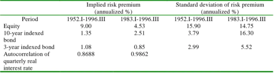
(14) 112. REVISTA ABANTE, VOL. 9, Nº 2. account portfolio must be even longer in order to achieve a full hedge. − With infinite risk aversion, it is possible to prove that the total return on virtual wealth at time t is rPt = rBt. (11). meaning that it is non-random when measured in future pension units (see Appendix 3). This quite remarkable since it implies that, when future contributions are known in advance, following the infinitely risk averse investment strategy guarantees at the beginning of the contribution period the pension level that will be obtained upon retirement. Finally, it is interesting to keep in mind that all of these results come simultaneously from a relatively simple model. Previously, some of these conclusions were obtained based on more complex and noble models, in other contexts. Our change in the numeraire allows us to obtain the results presented here. However, in contrast with Bodie, Merton and Samuelson (1992), and Campbell et al. (1999) or Bodie et al. (2004), in our case human capital volatility intervenes only through its covariance with eligible assets. The reason is that this volatility is assumed exogenous, and it is not affected by individual decisions. III. ORDERS OF MAGNITUDE IN ASSET DEMANDS AND FINAL PENSIONS. Campbell and Viceira (2001) calibrate a model of lifetime portfolio selection using historical US data for the term structure of interest rates and the aggregate stock market. They use a discrete time version of Vasicek (1977) with additional factors. Here we use only the equations and parameters related with the real term structure and the stock market. Appendix 4 repeats their equations and parameter values, which we use to estimate asset demands in our context as well as expected return and volatilities for human capital and the deferred pension. Table 2 shows a few important statistics. They estimate their model using quarterly data for the sample period 1956-1996, and also for the sub sample 1983-1996. Campbell and Viceira explain that for the latter period many authors have argued that.

(15) OPTIMAL PORTFOLIO IN DEFINED CONTRIBUTION. 113. real interest rates and inflation behave differently after the monetary-policy regime established since 1982 by Federal Reserve chairmen Volcker and Alan Greenspan. From our perspective, it is especially important to notice the persistence to the shocks to the short-term interest rate, reflected in the short-term autocorrelation. In the latter period it notably increases. If the autocorrelation coefficient is “large”, reversion to the mean in interest rates takes a longer time and thus reinvestment risk is more important, which should increase hedging demands for this motive. TABLE II IMPLIED PARAMETER ESTIMATES. Period Equity 10-year indexed bond 3-year indexed bond Autocorrelation of quarterly real interest rate. Implied risk premium (annualized %) 1952.I-1996.III 1983.I-1996.III 9.00 4.53 1.35 2.51 1.08 0.8688. 0.85 0.9862. Standard deviation of risk premium (annualized %) 1952.I-1996.III 1983.I-1996.III 15.90 14.75 3.79 16.30 2.99. 5.52. Source: Tables 1 and 2, Campbell and Viceira (2001), op cit. A. Asset demands. We assume that the future pensioner contributes to her individual account during 30 years. At the beginning, all of her virtual wealth is a 30year riskless bond, whose equal payments are sequentially passed to the individual pension account, which are then invested jointly with the rest of the accumulated wealth. We then assume a 20-year retirement period. Thus, at the beginning of the contribution years, the riskless asset is a pension deferred for 30 years which will pay for the following 20 years. For illustrative purposes, we assume that period by period the portfolio return is exactly its expected return, given the optimal portfolio weights at the beginning of each period (quarter). An important parameter is the “human capital” volatility relative to that of the deferred pension. Figure 1.A illustrates this relative volatility using Campbell and Viceira’s parameters for the period 1952-1996. We see that.

(16) 114. REVISTA ABANTE, VOL. 9, Nº 2. given its distant payments, the deferred pension has almost constant volatility during the entire period of contributions to the individual account. The relative human capital volatility decreases progressively, but stays between 0.9 and 0.8 during the first 20 years, decaying quickly during the last 10 years. However, these results change radically when considering a more recent period, depicted in Figure 1.B. For the period 1983-1996 the relative volatility barely surpasses 0.5 and drops much faster. Thus, for the rest of the analysis, we use the more recent parameter estimates, assuming they better represent the current behavior of interest rates. FIGURE 1 ABSOLUTE AND RELATIVE VOLATILITIES FOR “HUMAN CAPITAL” AND THE DEFERRED PENSION (Based on the parameters in Campbell and Viceira, 2001, Table 1, reproduced here in Table A4.1) A. 1953-1996. 0,025. 1 0,9 0,8 0,7 0,6. 0,015. 0,5 0,4. 0, 01. 0,3 0,005. 0,2 0,1. 0. 0 0. 2. 4. 6. 8. 10 12 14 16 18 20 22 24 26 28 30 Year σΚ. σΒ. σΚ/σΒ. Relat ive Vo latility. Quarter ly Volatili ty. 0, 02.

(17) OPTIMAL PORTFOLIO IN DEFINED CONTRIBUTION. 115. 0,6. 0,2 0,18. Quarter ly Volatility. B. 1983-1996. 0,14. 0,4. 0,12 0,3. 0,1 0,08. 0,2. 0,06 0,04. Relat ive Vo latility. 0,5. 0,16. 0,1. 0,02 0. 0 0. 2. 4. 6. 8. 10 12 14 16 18 20 22 24 26 28 30 Year σΚ. σΒ. σΚ/σΒ. Figure 2 shows the optimal invested proportions through time for different degrees of risk aversion. The figure for ??? corresponds to the logarithmic utility case, which only has the myopic component of asset demands. We appreciate that in that case the proportion invested in stocks is substantial. At the beginning, the net investment in the deferred pension is negative due to the human capital hedging component. Towards the end of the contribution period, the demand for the deferred pension becomes positive, but only due to its positive risk premium, since its Sharpe ratio improves. Here it is important to notice a complex problem: from a myopic perspective, initially the deferred pension appears as a dominated asset, given its very high volatility, being apparently less attractive than other asset classes. But by definition this does not consider the hedging benefits of very long-term bonds. This is something not easy to explain in a practical context..

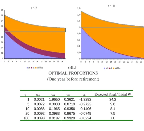
(18) 116. REVISTA ABANTE, VOL. 9, Nº 2. In the other cases, as expected, more risk aversion implies a higher proportion of total wealth (including human capital) invested in the deferred pension. In order to obtain the optimal proportions for the pension account we have to divide these numbers by one minus the relative importance of human capital, which substantially increases the demand for this asset, especially in the initial periods. In any case, under our assumptions the proportion of total wealth (including the present value of future contributions) invested in equity is constant. Table I shows the optimal invested proportions one year before retirement for different degrees of risk aversion. We see that the optimal investment in the deferred pension (or very long term real bonds) is still substantial one year before retirement. The portfolio duration is lengthened with short-term debt. Optimal investment in equity is probably overstated if it is true that historical returns for the period 1983-1996 in the US tend to overestimate expected returns. There is abundant evidence that this is so (see for example Fama and French (2002) or Dimson, Marsh and Staunton (2002)). FIGURE 2 PATH OF OPTIMAL PORTFOLIOS FOR DIFFERENT DEGREES OF RISK AVERSION (γ). αK is the proportion of human capital in the total “virtual wealth”; αB is the proportion in the deferred pension; αE the proportion invested in equity, and αρ the porportion invested in the short-term riskless asset. The X-axis is the year, which goes from 0 to 30.. γ=2. γ=1. 2,5. 3,5 3. 2. 2,5 1,5. 2 1. 1,5 1. 0,5. 0,5 0. 0. 0. 0. 2. 4. 6. 8. 10. 12 αΚ. 14 αΕ. 16 αΒ. 18 αρ. 20. 22. 24. 26. 2. 4. 6. 8. 10. 12. 14. 16. αΚ. αΕ. αΒ. 18. 28 αρ. 20. 22. 24. 26. 28.

(19) OPTIMAL PORTFOLIO IN DEFINED CONTRIBUTION. 117. γ = 10 0. γ = 10. 1,6. 1,8 1,6. 1,4. 1,4. 1,2. 1,2. 1. 1. 0,8. 0,8. 0,6 0,6. 0,4. 0,4. 0,2. 0,2 0. 0 0. 2. 4. 6. 8. 10. 12. 14. 16. αΚ. αΕ. αΒ. γ 1 5 10 20 100. 18 αρ. αK 0.0021 0.0072 0.0085 0.0092 0.0098. 20. 22. 24. 26. 28. 0. 2. 4. 6. 8. TABLE III OPTIMAL PROPORTIONS (One year before retirement) αS 1.9650 0.3930 0.1965 0.0983 0.0197. αΒ 0.3621 0.8719 0.9356 0.9675 0.9929. 10. 12. 14. 16. 18. αΚ. αΕ. αΒ. αρ. 20. 22. 24. 26. 28. Expected Final / Initial W αr -1.3292 34.2 -0.2722 9.6 -0.1406 8.1 -0.0749 7.5 -0.0224 7.0. B. Final pension confidence intervals. Using the same information as above and assuming the optimal investment path for a given level of risk tolerance, we obtain confidence intervals for the final pensions per unit of present value of future contributions (or “human capital”). Given our assumptions, the variance of the final pension simply corresponds to the sum of the one-period tracking error variances, which gives us the critical input for the confidence interval. Results are illustrated in Figure 3. and presented in Table III It shows that only for very little risk tolerance the confidence interval is relatively tight. On the other hand, for log utility the upper (90 percent) confidence interval limit is 200 times that of the lower limit (10 per cent) whereas for a risk aversion level of 10 the ratio is about 1.7 times. This is a rather uncomfortable conclusion since in order to have relatively predictable final pensions per unit of present value of future contributions, a very large fraction of total wealth should be invested in very long term bonds, which in turn exhibit very high short term volatility..

(20) 118. REVISTA ABANTE, VOL. 9, Nº 2. FIGURE 3 FINAL PENSION CONFIDENCE INTERVAL FOR DIFFERENT DEGREES OF RISK TOLERANCE (1/γ) The figure shows a 90 percent confidence interval for the final pension as a fraction of the present value of the future contributions (or “human capital”, HK). For each level of risk tolerance the optimal investment path is assumed to be followed.. F inal pension per un it of HK. 10. 1. 0,1. 0,01 0. 0,2. 0,4. 0,6. 0,8. 1. Risk T oler ance (1/γ) 10%. Mean. 90%. IV. POLICY IMPLICATIONS OF THESE RESULTS. The above results have several practical or policy implications for defined contribution pension funds, including, of course, for mandatory systems, which started with the Chilean reform in 1981. First, the definition of risk has to be revised. Risk is not short-term volatility. For example, using the parameters of the previous section, halfway to retirement the deferred pension is twice as volatile as equity. Thus, even though this asset guarantees by definition a future pension, its short-.

(21) OPTIMAL PORTFOLIO IN DEFINED CONTRIBUTION. 119. term volatility measured at market prices will appear to be extreme. From here it is evident that measuring risk using Value at Risk or VaR for defined contribution pension systems (as it is currently done in Mexico), makes little sense and may be counterproductive, since it provides incentives to invest in short-term fixed income. Short-term instruments are obviously not good hedges against future increases in pension costs. In other words, VaR considers only the myopic part of asset demands, and not their hedging component. Second, it is evident that the most important state variable in this context is the level of the local long term real interest rates upon retirement. This means that even defined contribution pension funds should find a preferred habitat in very long-term inflation-indexed fixed rate local bonds, since these instruments are the best hedge against adverse changes in retirement annuity costs, caused by drops in the long-term real interest rates. The policy implication of this is that developing a long-term indexed local bond market should be an important complement to pension reforms based on defined contribution individual accounts. Third, the stochastic processes followed by emerging market real interest rates are key determinants of the importance of reinvestment risk. The faster interest rates revert to their long-term means, the lower the relative importance of reinvestment risk. However, given that emerging markets are often small and open economies, local monetary policies should be less relevant than international factors (such as interest rate levels and risk premia) for determining these stochastic processes. Finally, it is interesting to notice that changes in local long-term real interest rates are likely to have higher correlation with local rather than with international equity returns. This means that the hedging component of asset demands should exhibit home bias.4 However, if indeed salaries and local aggregate dividends are cointegrated, these conclusions may be partly reversed. Naturally, the myopic component of asset demands will probably favor international investments, given lower total risk and eventually higher Sharpe ratios.. 4. See Walker (2003)..

(22) 120. REVISTA ABANTE, VOL. 9, Nº 2. V. CONCLUSIONS. We have developed a relatively simple model, in the spirit of Campbell and Viceira (2001), which solves the portfolio problem for a defined contribution pension fund. For this purpose we assume that the future contributions to the individual pension account are predictable and thus their present value behaves like a bond. We further assume that upon retirement, the pensioner buys an annuity with her total accumulated savings. The pension fund manager must find asset allocations that maximize through time the expected pension level given its risk. As in other studies, assuming constant risk premia, correlations and volatilities but stochastic interest rates, asset demands have a myopic component and also hedging components. In our case, hedging against drops in long-term local real interest rates is desirable, since it implies lower pensions for a given level of accumulated wealth. One practical implication of our results is that even after assuming that interest rates are stochastic with mean reversion, and the existence of “human capital”, the portfolio problem can be solved one period at a time, measuring expected returns and risk in units of the future pension. Our results are evaluated using the parameters estimated by Campbell and Viceira (2001) for the Unites States. We conclude that with moderate levels of risk aversion a significant fraction of total wealth should be invested in very long-term bonds (or in the deferred pension, in our case), even when little time is left for retirement. Moreover, the effect of considering future contributions to the individual pension account as part of the portfolio problem is to increase further these hedging demands. The intuition behind this is that if all wealth were in the individual account, an infinitely risk averse investor would want all of it invested in the deferred pension. Given that a future contributions are equivalent to holding fraction of total wealth as a “bond in a parallel account”, with lower duration, the duration of investments in the pension fund account should be lengthened further to compensate for this. We thus reiterate Campbell and Viceira’s (2002) conclusion for the case of defined contribution (possibly mandatory) pension system asset allocations, that pension funds should hold very long term bonds, but they should be denominated in local real currency..

(23) OPTIMAL PORTFOLIO IN DEFINED CONTRIBUTION. 121. REFERENCES Bajeux-Besnainou, I., J.V. Jordan and R. Portait (2003). Dynamic Asset Allocation for Stocks, Bonds and Cash, Journal of Business 76(2): 263-288. Benzoni, L, P. Collin-Dufresne and R. S. Goldstein (2006). Portfolio Choice over the LifeCycle when the Stock and Labor Markets are Cointegrated. Forthcoming in Journal of Finance. Bodie, Z. (2001). Retirement Investing: A New Approach. Pension Research Council Working Paper 2001-8. Bodie, Z. (2002). An Analysis of Investment Advice to Retirement Plan Participants, Pension Research Council, Working Paper, 2002-15. Bodie, Z. (2002). Life-Cycle Finance in Theory and in Practice. Boston University School of Management Working Paper 2002-02. Bodie, H. y Mitchell. (2000). A Framework for Analyzing and Managing Retirement Risks. PRC WP 2000-4. Bodie, Z., R. Merton and W. Samuelson. (1992). Labor supply flexibility and portfolio choice in a life cycle model. Journal of Economic Dynamics and Control 16: 427-449. Bodie, Z., J. Detemple, Su. Otruba and S. Walter (2004). Optimal consumption-portfolio choices and retirement planning. Journal of Economic, Dynamics and Control, 28: 1115-1148. Campbell, J. and L. Viceira. (2001). Who should buy long-term bonds? American Economic Review, 91(1): 99-127. Campbell, J., J. Cocco, F. Gomes, and P. Maenhout (2001). Investing Retirement Wealth: A Life-Cycle Model, in John Y. Campbell and Martin Feldstein eds., Risk Aspects of Investment-Based Social Security Reform, University of Chicago Press: Chicago, IL, 439473. Campbell, J. and L. Viceira. (2002). Strategic Asset Allocation: Portfolio Choice for LongTerm Investors First Edition; Oxford University Press Inc., New York. Campbell, J., G. Chacko, J. Rodríguez and L. Viceira. (2004). Strategic Allocation in a Continuous Time VAR Model. Journal of Economics, Dynamics and Control, 28: 21952214. Carroll, C. (1997). Buffer-Stock Saving and the Life Cycle/Permanent Income Hypothesis, Quarterly Journal of Economics, 1-55. Carroll, C. (2001). A Theory of The Consumption Function, With and Without Liquidity Constraints. Journal of Economic Perspectives 15(3): 23-45. Cocco, J., F. Gomes and P. Maenhout. (2005). Consumption and Portfolio Choice over the Life Cycle. Review of Financial Studies, 18, 2: 491-533. Cocco, J. (2005). Portfolio Choice in the Presence of Housing. Review of Financial Studies, 18(2): 535-567. Constantinides, G. (1984). Optimal Stock Trading with Personal Taxes: Implications for Prices and the Abnormal January Returns. Journal of Financial Economics 13: 65-89. Dimson, E., P. Marsh and M. Staunton (2002). Triumph of the Optimists. 101 years of global investment returns. Princeton University Press. Esposito, M. (2003). Life-Cycle Investing: A practitioners point of view. Mimeo. Faig, M. and P. Shum (2002). Portfolio Choice in the presence of Personal Illiquid Projects. Journal of Finance, 57(1):303-328. Fama, E. F. and Kenneth R. French (2002). The equity premium, Journal of Finance. April 2002, 57(2): 637-659. Jagannathan, R. and Z. Wang. (1996). The Conditional CAPM and the Cross-Section of Expected Returns. Journal of Finance, 51: 259-299. Merton, R. (1971). Optimum Consumption and Portfolio Rules in a Continuous-Time Model. Journal of Economic Theory, 3: 373-413. Merton, R. (2000). Continuous Time Models in Finance. Blackwell. Samuelson, Paul A. (1969. Lifetime Portfolio Selection by Dynamic Stochastic Programming. Review og Economics and Statistics 51: 239-246..

(24) 122. REVISTA ABANTE, VOL. 9, Nº 2. Siegel, J. (1998). Stocks for the long run, Second Edition; Mc Graw-Hill. Thaler, R. (1985). Mental accounting and consumer choice. Marketing Science, 4: 199-214. Vasick, O. (1977). An Equilibrium Characterization of the Term Structure. Journal of Financial Economics, 5: 177-178. Viceira, L. (2001). Optimal Portfolio Choice for Long-Horizon Investors with Non tradable Labor Income. Journal of Finance, 56(2): 433-470. Walker, E. (2002). Multifondos y falacias: ¿Se habrá puesto la carreta delante de los bueyes? Administración y Economía UC. N° 48. Walker, E. (2003). Determinación de la cartera de inversión óptima de una AFP. Mimeo. Wang, X. (2002). Income Risk and Portfolio Choice: An Empirical Study. Ohio State University..

(25) OPTIMAL PORTFOLIO IN DEFINED CONTRIBUTION. 123. APPENDIX 1 INTERTEMPORAL OPTIMIZATION. Result for T-1 Using the definitions given in the text, 2 −α rPT = rT + α KT −1(rKT − rT ) + 1 α KT −1(1 − α KT −1 )σ KT KT −1α'T −1 σ K •T 2 + α'T −1 (ρT − rT ι) + 1 α'T −1 ΛT − 1 α'T −1 ΣT αT −1 2 2. (A1.1). we get. 2 2 2 varT −1(rPT − rBT ) = αKT −1σ KT + 2αKT−1α'T −1 σ K•T + α'T −1 ΣαT −1 − 2ααT −1 σ B•T + σ BT. (A1.2) The derivative of the expected return with respect to α T −1 is dET −1rPT = ET −1(ρT − rT ι) + 1 ΛT − ΣT αT −1 − α KT −1σ K •T 2 da' T −1. (A1.3). The derivative of the second term of the objective function is. 1 (1 − 2. γ). dvarT −1 (rPT − rBT ) 1 = 2 (1 − γ)(2Σ T αT + 2α KT −1σ K •T − 2σ B •T ) (A1.4) da'T −1. Equating the sum of both to zero gives the solution:. αT* −1 = 1γ ΣT−1 ET −1 (ρT − rT ι + 12 ΛT ) − α KT −1 ΣT−1σ K •T + (1 − 1γ )ΣT−1σ B•T. (A1.5). Result for T-2 dV T − 2 = ET − 2 (ρT −1 − rT −1ι) + 12 ΛT −1 − Σ T −1αT − 2 − α KT − 2 σ K •T −1 + (1 − γ)(Σ T αT + α KT −1σ K •T − σ B•T ) dααT − 2 + (1 − γ). (. ). d d * * covT − 2 (rPT −1 − rBT −1 ,rPT − rBT ) + 12 (1 − γ) varT − 2 ET −1 (rPT − rBT ) = 0 dααT − 2 dααT − 2.

(26) 124. REVISTA ABANTE, VOL. 9, Nº 2. αT* − 2 = 1γ ΣT−−11 ET − 2 (ρT −1 − rT −1ι + 21 ΛT −1 ) − α KT − 2 ΣT−−11σ K •T −1 + (1 − 1γ )ΣT−−1 1σ B•T −1 ⎛ d * * rPT + (1 − γ)ΣT−−11 ⎜⎜ covT − 2 (ρPT −1 , rPT − rBT ) + covT − 2 (rPT −1 − rBT −1 , dα T −2 ⎝ ⎛ d * * rPT ), ET −1 (rPT + 2(1 − γ)ΣT−−11covT − 2 ⎜⎜ ET −1 ( − rBT dαT − 2 ⎝. ⎞ ) ⎟⎟ ⎠. (A1.6). ⎞ ) ⎟⎟ ⎠. To analyze the order of magnitude of the approximation error of ignoring the last two terms, it is useful noticing that * * rPT ≈ rPT (α KT − 2 ) + (rKT − rT + C T − 2 )(α KT −1 − α KT − 2 ) where C T-2 is a small. constant from the perspective of T-2. This approximation is obtained as follows: * * rPT ≈ rPT (α KT − 2 ) +. * drPT (α KT − 2 ) (α KT −1 − α KT − 2 ) dα KT −1. * 2 rPT (α KT −2 ) = rT + α KT − 2 (rKT − rT ) + 12 α KT − 2 (1 − α KT −1 )σ KT − α KT − 2 α'T −1 σ K •T. + α'T −1 (ρT − rT ι) + 12 α'T −1 ΛT − 21 α'T −1 Σ T αT −1. (A1.7). (A1.8). On the other hand,. drPT (α KT −2 ) = (rKT − rT ) + CT −2 dα KT −1. (A1.9). where CT-2 is nonrandom form the perspective of T-2. Thus * * rPT ≈ rPT (α KT − 2 ) + (rKT − rT + CT − 2 )(α KT −1 − α KT − 2 ). (A1.10). Using A1.10 en A1.6, we see that the covariances will either be small or zero, especially if the portfolio is updated frequently. Indeed, * cov T − 2 (ρ PT −1 , rPT − rBT ) is close to zero since risk premia are not predict-. able. Also,.

(27) OPTIMAL PORTFOLIO IN DEFINED CONTRIBUTION. covT − 2 (rPT −1 − rBT −1 ,. 125. d dα * rPT ) = covT − 2 (rPT −1 − rBT −1 ,(rKT − rT ) KT −1 ) dαT − 2 dαT − 2. is approximately zero because K’s risk premium is unpredictable and the indirect impact on the relative importance of human capital is small. Finally,. ⎛ d * * rPT ), ET −1 (rPT covT − 2 ⎜⎜ ET −1 ( − rBT dαT −2 ⎝. ⎞ ) ⎟⎟ ⎠. is. ⎛ dα * − rBT covT −2 ⎜⎜ ET −1 (rKT − rT ) KT −1 , ET −1 (rPT dαT −2 ⎝. ⎞ ) ⎟⎟ ⎠. which again is approximately equal to zero given that the risk premia are not predictable..

(28) 126. REVISTA ABANTE, VOL. 9, Nº 2. APPENDIX 2 EVOLUTION OF THE RELATIVE IMPORTANCE OF “HUMAN CAPITAL”. Here we search for an approximate relationship between the relative importance of human capital in two successive periods. By definition, we have α Kt =. K tT K exp(r Kt ) − C = t −*1T = α Kt − 1 exp(r Kt − rPt − c t ) + 1 − exp(c t ) * Wt W t − 1 exp(r Pt ) + C. (A2.1). where c t ≡ log(1 + C / Wt*−1 exp(rPt )) Using a first order Taylor series expansion, we get α Kt − α Kt −1 ≈ α Kt −1 (rKt − rPt − ct ) − ct. (A2.2). dα Kt 2 1 = α Kt −1 σ K • t − α Kt −1 (ρt − rt ι + 2 Λt ) + 2α Kt −1 Σ T αt −1 da' t −1. (A2.3). Thus. dα Kt = (α Kt − 2 (1 + rKt −1 − rPt −1 − ct −1 ) − ct −1 )2 σ K •t da' t −1 − (α Kt − 2 (1 + rKt −1 − rPt −1 − ct −1 ) − ct −1 )(ρt − rt ι + 21 Λt ) + 2(α Kt − 2 (1 + rKt −1 − rPt −1 − ct −1 ) − ct −1 )Σ T αt −1. (A2.4).

(29) OPTIMAL PORTFOLIO IN DEFINED CONTRIBUTION. 127. APPENDIX 3 RETURN OF THE INFINITELY RISK AVERSE PORTFOLIO. 2 2 2 rPt = rt + α Kt −1 (rKt − rt + 12 σ Kt ) − 21 α Kt −1σ Kt − α Kt −1α' t −1 σ K •t + α' t −1 (ρt − rt ι). + 12 α' t −1 Λt − 12 α' t −1 Σ t αt −1. 2 2 2 2 rPt = rt + α Kt −1 (rKt − rt + 12 σ Kt ) − 21 α Kt −1σ Kt − α Kt −1 (1 − υt α Kt −1 )υt σ Bt + (1 − υt α Kt −1 )(rBt − rt ). + υt ≡. 1 2. (1 − υt α Kt −1 )σ Bt2 − 12 (1 − υt α Kt −1 )2 σ Bt2. σ Kt σ Bt. 2 2 rKt = rt − 21 σ KT + υt (rBt + 21 σ Bt − rt ). 2 2 2 2 rPt = rt + α Kt −1υt (rBt + 21 σ Bt − rt ) − 21 α Kt −1σ Kt − α Kt −1 (1 − υt α Kt −1 )υt σ Bt + (1 − υt α Kt −1 )(rBt − rt ). +. 1 2. (1 − υt α Kt −1 )σ Bt2 − 12 (1 − υt α Kt −1 )2 σ Bt2. rPt = rBt. APPENDIX 4 MODEL AND PARAMETERS OF CAMPBELL AND VICEIRA (2001). Campbell and Viceira (2001) assume a stochastic discount factor (SDF) (Mt) with a log-normal distribution, where xt = -Etmt+1 follows an AR process (with also implies mean reversion). Let mt = log(Mt), they assume. − mt +1 = xt + vmt + 1 xt +1 = (1 − φx )μ x + φx xt + ε xt +1 vmt +1 = βmx ε xt +1 + ε mt +1. This means that the short-term interest rate is determined as follows: The negative of the logarithm of a zero-coupon bond price is 2 rt + 1 = xt − 12 (β mx σ x2 + σ m2 ).

(30) 128. REVISTA ABANTE, VOL. 9, Nº 2. The negative of the logarithm of zero-coupon price is − p nt = An + B n xt. where. Bn = 1 + φ x Bn −1 =. 1 − φ xn 1 − φx. An − An −1 = (1 − φx )μ x Bn −1 −. 1 2. [(β. mx. + Bn −1 )2 σ x2 + σ m2. ]. with A0 = B0 = 0. The observed and expected return on a zero coupon bond are, respectively, rnt +1 − rt +1 = − 21 Bn2−1 − βmx Bn −1σ x2 − Bn −1 ε xt +1 Et (rnt +1 − rt +1 ) + 21 vart (rnt +1 − rt +1 ) = − βmx Bn −1σ x2. For the return of the equity market, (re) they assume ret +1 − Et ret +1 = βex ε xt +1 + βem εmt +1. and the risk premium with respect to the short term interest rate is: Et ret +1 − rt +1 + 12 vart (ret +1 − rt +1 ) = β mx βex σ x2 + βem σ m2.

(31) OPTIMAL PORTFOLIO IN DEFINED CONTRIBUTION. TABLE AIV-1 PARAMETERS FOR THE REAL TERM STRUCTURE OF INTEREST RATES AND THE EQUITY MARKET. 1952:1-1996:3 1983:1 -1996:3 Parameter Estimate Std Error Estimate Std Error ?x 0.0573 0.0298 0.0194 0.0693 0.8688 0.0057 0.9862 0.0042 ?x -74.9797 41.6949 -28.6919 114.0025 ? mx -3.4957 3.4123 -9.3629 6.3014 ? ex 0.3013 0.0979 0.5089 1.3528 ? em 0.0025 0.0001 0.0027 0.0006 ?x 0.2694 0.0927 0.1351 0.3579 ?m Source: Campbell and Viceira (2001), Table 1. 129.

(32)