TítuloInverse problem of water flow and reactive solute transport in variably saturates porous media

Texto completo

(1)^,^ ._. P ^ ^. ^ ^ ^ ^. ^^ ^. •.. 9w, ^. i ^ ^.^,^^. u. 1. s. r^.. ` r^ei^. ;• ^. '^. j"::. ^. `^. ,^. ^. ^. >^. •. ^. 11^. .. ^. ^• Y (^ t.. ^ aa , ;;^. 'f. ^. ^. ^^. ^k. ^. ^. ^. • 1:. `^ - ^. .. ^. ^. ^. ^. ® ^lir. b. ^. ^'. ^.. t. ^. J^^. '^^^. .-,i.. ^,. :^ ^ :^. ^.r. ,. ^^. ^ . w., ^ ,. ^. a^. r:. ^. `. ^. _ ,^. ^ = },^. ^^. ^'s. ^ r:f. s. ^,. `. ^` t. R. 8• .. ^. ti ^«,. ^ i. S. ,. '. _. :. ^. ^^. •,. ,^. ^. •. ^f^. ^. ^^^.

(2) ^ , ^9C -,t^^t M. UNIVERSITY OF LA CORUNA CIVIL ENGINEERING SCHOOL DEPARTMENT OF CONSTRUCTION TECHNOLOGY. INVERSE PROBLEM OF WATER FLOW AND REACTIVE SOLUTE TRANSPORT IN VARIABLY SATURATED POROUS MEDIA. Ph.D. Dissertation by ZH ENXU E DAI as partial fulfillment of Ph.D. requirements within the Civil Engineering Ph.D. Program. Advisor: JAVIER SAMPER CALVETE University of La Coruña. La Coruña. October, 2000.

(3) Department of Construction Technology Civil Engineering School. University of La Coruña. INVER SE PRO B LEM OF WATER FL OW AN D REACTIVE SOLUTE T RANSPORT I N VARIABLY SATURATED P O ROUS MEDIA. Ph.D. Dissertation Submitted by ZHENX UE DAI as partial fulfillment of Ph. D requirements within the Civil Engineering Ph.D. Program. Advisor: JAVIER SAMPER CALVETE, University of La Coruña. La Coruña. October, 2000.

(4) Departamento de Tecnología de la Construcción Escuela Técnica Superior de Ingenieros de Caminos, Canales y Puertos Universidad de La Coruña ^. EL PROBLEMA INVER SO DEL FLU J O D E AGUA Y EL TR ANSPORTE DE SOLUTOS R EACTIVOS EN MEDI OS P O ROSOS PARCIALMENTE SATU RAD OS. Tesis Doctoral Presentada por. ZHENX UE DAI Para cumplir los requisitos del Programa de Doctorado en Ingeniería Civil. Dirigida por: JAVIER SAMPER CALVETE, Universidad de La Coruña. La Coruña - Octubre de 2000.

(5) RESUMEN. 1. RES UMEN. El estudio de la calidad química de las aguas subterráneas y la cuantificación de su contaminación, así como la evaluación de los efectos que producen los almacenamientos de residuos en el subsuelo requiere el uso de modelos numéricos. Estos modelos deben considerar conjuntamente el flujo de agua, el transporte de calor y de especies disueltas, junto con sus complejas interacciones con las fases sólidas y gaseosas. En esta tesis se presenta una formulación matemática y numérica para resolver el problema inverso del flujo de agua, transferencia de calor y transporte de un sistema multicomponente de solutos reactivos en medios parcialmente saturados.. Se han desarrollado tres códigos que resuelven el problema inverso basándose en tres métodos diferentes: método de la. sección áurea, interpolación cuadratica y Gauss-NewtonLevenverg-Marquardt. Los dos primeros no requieren calcular el Jacobiano y son especialmente apropiados para resolver problemas con pocos parámetros. Sin embargo, para más de diez parámetros estos métodos no son eficientes y se debe de recurrir al método de Gauss-Newton-Levenverg-Marquardt que es más potente, robusto y eficiente que los otros dos. Este método requiere calcular las derivadas de las variables (niveles, concentraciones, caudales y contenido de humedad) con respecto a los parámetros del modelo. Para ello se utiliza un método de diferencias finitas (esquema hacia adelante y centrado). Para parámetros que varían en escala logarítmica el código realiza una transformación logarítmica que generalmente aumenta la velocidad de convergencia y proporciona valores no negativos. Para evaluar la precisión de" los parámetros estimados, el código calcula el error de los valores estimados, así como medidas estadísticas de la bondad del ajuste. También proporciona la matriz de varianza-covarianza y la de correlación de los parámetros estimados, los autovalores y autovectores de la matriz de covarianza, así como la aproximación de los intervalos de confianza de los parámetros estimados. Todo esto se ha incorporado en la versión final del código INVERSE-CORE2D, que incluye el modelo directo e inverso. El modelo directo esta basado en CORE2D (Samper et al., 1999) e incluye: 1) Flujo de agua en 2D, confinado o no confinado, saturado o no saturado,.

(6) INVERSE PROBLEM OF REACTNE SOLUTE TRANSPORT. 11. estacionario o transitorio y con condiciones de contorno generales, 2) Transporte de calor transitorio debido a procesos de conducción, dispersión y convección, 3) Transporte de solutos por procesos de advección, difusión molecular y dispersión hidrodinámica, 4) Reacciones químicas: acido-base, redox, complejación acuosa, adsorción, intercambio ionico, disolución/precipitación de minerales, disolución/exolución de gases y 5) Desintegración radiactiva.. Para resolver el problema inverso se tienen en cuenta cinco tipos de datos; niveles piezométricos, concentración de especies químicas, concentración total en fase liquida y sólida, caudales y contenido de humedad, así como información previa de los parámetros. Los datos se generalizan por medio de coeficientes de peso. INVERSE-CORE2D permite la estimación de los siguientes parámetros de flujo y transporte de solutos reactivos, los cuales pueden variar para cada zona de material del modelo: 1) porosidad total, 2) conductividad hidráulica saturada (KX y Ky), 3) coeficiente de almacenamiento, 4) los parámetros m, n, y a de las curvas de retención y las funciones de permeabilidad relativa, 5) coeficiente de difusión molecular, 6) dispersividad, 7) coeficiente de reparto, 8) porosidad accesible, que difiere de la total en el caso de considerar exclusión anionica, 9) concentraciones iniciales de las especies químicas incluyendo pH y pE, 10) concentraciones de contorno de las especies químicas, 11) coeficientes de selectividad para el intercambio cationico, 12) capacidad de ^ cambio de los cationes (CEC), 13) superficie especifica de los minerales, 14) energía de activación de las reacciones controladas cinéticamente, 15) constantes cinéticas, y 16) los exponentes del efecto catalítico y del estado de saturación en la ecuación cinética que define la velocidad de disolución/precipitación de minerales.. Se han utilizado tres series de datos sintéticos para verificar la convergencia, unicidad y estabilidad del algoritmo inverso. Estos ejemplos muestran que la existencia de información previa de los parámetros reduce la covarianza y la correlación entre parámetros, reduciendo, por tanto, la incertidumbre en esos parámetros. La incorporación de la información previa mejora también la eficiencia del proceso de estimación. Los códigos que resuelven el problema inverso se han utilizado satisfactoriamente para interpretar diferentes tipos de experimentos de laboratorio: 1) infiltración, 2) difusión y 3) flujo "a través" en bentonitas y granitos, en los que los parámetros de flujo y transporte se.

(7) RESUMEN. 111. han estimado bajo diferentes condiciones. Un experimento en columna, publicado por Appelo et al. (1990), ha sido utilizado para examinar la metodología inversa en un problema real de transporte reactivo. Se estimaron los valores de la dispersividad, coeficientes de selectividad, CEC, así como de las concentraciones iniciales y de contorno de los principales componentes qufmicos. La solución del problema inverso fue de gran utilidad para la identificación de los procesos geoquímicos más relevantes que tienen lugar durante el experimento.. Esta metodología se aplicó también a dos casos de campo, el acuítardo del Delta del Llobregat (Barcelona) y el acuífero de Aquia (Maryland, USA). En ambos casos se produce una mezcla de agua salada con agua dulce. Los valores de la conductividad hidráulica, dispersividad, coeficientes de selectividad, CEC y concentraciones iniciales y de contorno de los principales componentes químicos se estimaron satisfactoriamente para diferentes hipótesis sobre las condiciones redox. Los resultados de la estimación indican que los procesos redox son procesos geoquímicos importantes en el acuítardo del Delta del Llobregat. Además, se ha cuantificado la incertidumbre asociada a los parámetros y se han calculado los intervalos de confianza aproximados.. En general, los resultados obtenidos con los ejemplos sintéticos y los casos reales indican que INVERSE-C^REZD es una herramienta de optimización flexible y robusta para resolver el problema inverso de flujo y transporte de solutos reactivos..

(8) INVERSE PROBLEM OF REACTNE SOLUTE TRANSPORT. N.

(9) ABSTRACT. Understanding natural groundwater quality patterns, quantifying groundwater pollution and assessing the effects of waste disposal require modeling tools accounting for water flow, and transport of heat and dissolved species as well as their complex interactions with solid and gaseous phases. This dissertation presents a mathematical and numerical methodology for solving the coupled inverse problem of water flow, heat transfer and multicomponent reactive solute transport in variably saturated media.. Three inverse codes have been developed which are based on: (1) Golden section search, (2) quadratic interpolation, and (3) Gauss-Newton-Levenverg-Marquardt method. The first two methods do not require computing the Jacobian matrix. They are especially suited for the estimation of a few parameters. They are not efficient for problems involving more than ten parameters. In such cases, one must resort to the Gauss-Newton-LevenbergMarquardt method which is more powerful, robust and efficient. The latter is a gradientbased optimization algorithm in which derivatives of observations (heads, solute concentrations, total concentrations, cumulative water inflow and water content) with respect to model parameters are calculated using either forward or central fuúte differences. For possitively-valued parameters and for those which vary in a logarithmic scale the code performs a log transformation which generally enhances the rate of convergence and ensures non-negative estimates. To evaluate the accuracy of the estimated parameters, the code computes parameter estimation errors and statistical measures of goodness-of-fit. It also computes the covariance and correlation matrices of the estimated parameters, the eigenvalues and eigenvectors of the covariance matrix, as well as approximate confidence intervals of the estimated parameters. All these features are incorporated in INVERSECORE2D, the most updated and complete of the three inverse codes. The forward modeling part of INVERSE-CORE2D is entirely based on CORE2D , a code developped at the University of La Coruña by Samper et al. (1999) which accounts for: 1) 2-D confined or unconfined, saturated or unsaturated steady or transient groundwater flow with general boundary conditions, 2) Transient heat transport including conduction, heat dispersion and.

(10) INVERSE PROBLEM OF REACI'NE SOLUTE TRANSPORT. VI. advection processes, 3) Solute transport including advection, molecular diffusion and mechanical dispersion, 4) Chemical reactions including: acid-base, redox, aqueous complexation, surface adsorption, ion exchange, mineral dissolution-precipitation, gas dissolution-exsolution, and retardation, and 5) Radioactive decay.. Up to five different types of data can be taken into account for the solution of the inverse problem, including: hydraulic heads, concentrations of dissolved chemical components, total concentrations (including liquid and solid phases), water fluxes and water contents, as well as parameter prior information. These data have been generalized in a weighted least square criterion by a set of weighting coefficients. INVERSE-CORE2D can estimate a wide range of flow and reactive transport parameters which may be different in different parameter zones. These parameters include: 1} total porosity, 2) components of the saturated hydraulic conductivity (KX and Ky), 3) specific yield, 4) parameters m, n, and a which are used for defining retention curves and relative permeability functions, 5) molecular diffusion coefficient, 6) solute dispersivity, 7) distribution coefficient Kd of a sorbing chemical, 8) accessible porosity, which may differ from total porosity when anion exclusion takes place, 9} initial concentrations of chemical components, including initial pH and pE, 10) boundary concentrations of chemical components, 11) selectivity coefficients of cation exchange, 12) cation exchange capacity (CEC), 13) specific surface of minerals, 14) apparent activation energy of kinetically-controlled reactions, 15) kinetic rate constant, and 16) exponents of catalytic terms and those of the ratio of the ionic activity products and the equilibrium constants for kinetically-controlled mineral dissolution/precipitation.. Three sets of synthetic data have been used to verify the codes and study the convergence, uniqueness and stability of the inverse algorithms. These examples illustrate that. parameter. prior information reduces parameter correlation. and uncertainty.. Incorporating prior information leads also to a significant improvement of the numerical efficiency of the estimation process.. ^. The inverse codes developped in this dissertation have been successfully used to interpret different types of laboratory experiments. Infiltration, diffusion, and permeation experiments in bentonite and granite have been used to estimate flow and transport.

(11) ABSTRACI. VII. parameters. A column experiment reported by Appelo et al. (1990) has been used to test the inverse methodology on reactive transport data. Solute dispersivity, selectivity coefficients, CEC, and initial and boundary concentration of the main chemical components have been estimated. The solution of the inverse problem was useful in this case for identifying relevant geochemical processes taking place during the experiment. The methodology has also been applied to field case studies at the Llobregat Delta Aquitard (Barcelona, Spain) and the Aquia aquifer (Maryland, USA). Both of them deal with salt water leaching with fresh water. Hydraulic conductivities, dispersivities, selectivity coefficients, CEC, initial and boundary concentrations of the main chemical components were successfully estimated for different redox hypotheses. Estimation results indicate that redox processes are important geochemical processes in the Llobegat Delta aquitard. The uncertainty of the estimated parameters has been quantified and approximate confidence intervals were computed.. Overall, the results obtained with synthetic and real examples indicate that INVERSECORE2D is a flexible and robust optimization tool for the solution of the inverse problem of flow and reactive solute transport..

(12) INVERSE PROBLEM OF REACTNE SOLUTE TRANSPORT. Vlll.

(13) RESUMO. IX. RESUMO. O estudio da calidade química das augas subterráneas e a cuantificación da súa contaminación, así como a avaliación dos efectos que producen os almacenamentos de refugallos no subsuelo require o uso dos modelos numéricos. Estos modelos deben considerar conxuntamente o fluxo da auga, o transporte da calor e das especies disoltas, xunto coas súas complexas interaccións coas fases sólidas e gaseosas. Nesta tese de doutoramento preséntase unha formulación matemática e numérica ^ para resolve-lo problema inverso do fluxo de auga, transferencia da calor e transporte dun sistema multicomponente dos solutos reactivos nos medios parcialmente saturados.. Desenroláronse tres códigos que resolven o problema inverso baseándose en tres métodos diferentes: método da sección áurea, interpolación cuadrática e Gauss-NewtonLevenverg-Marquardt. Os dous primeiros non requiren calcula-lo Jacobiano e son especialmente apropiados para resolve-los problemas con poucos parámetros. Sen embargo, para máis de dez parámetros estos métodos non son eficientes e débese recurrir 6 método de Gauss-Newton-Levenverg-Marquardt que é máis potente, robusto e eficiente que os outros. dous.. Este. método require calcula-las. derivadas. das. variables. (niveis,. concentracións, caudais e contido de humidade) con respecto ós parámetros do modelo. Para isto utilízase un método de diferencias finitas (esquema hacia diante e centrado). Para parámetros que varían na escala logarítmica o código realiza unha transformación logarítmica que xeralmente aumenta a velocidade da convergencia e proporciona valores non negativos. Para evalua-la precisión dos parámetros estimados, o código calcula o erro dos valores estimados, así como as medidas estadísticas da bondade do axuste. Tamén proporciona a matriz da varianza-covarianza e a da correlación dos parámetros estimados, os autovalores e autovectores da matriz de covarianza, así como a aproximación dos intervalos de confianza dos parámetros estimados. Todo isto incorporouse na versión final do código INVERSE-CORE2D, que inclúe o modelo directo e inverso. O modelo directo básase no CORE2D (Samper et al., 1999) e inclúe: 1} Fluxo de auga en 2D, confinado ou non confmado, saturado ou non saturado, estacionario ou transitorio e con condicións de.

(14) INVERSE PROBLEM OF REACTNE SOLUTE TRANSPORT. X. contorno xerais, 2) Transporte da calor transitorio debido a procesos de conducción, dispersión e convección, 3) Transporte de solutos por procesos de advección, difusión molecular e dispersión hidrodinámica, 4) Reaccións químicas: ácido-base, redox, complexación acuosa, adsorción, intercambio iónico, disolución/precipitación de minerais, disolución/exolución de gases e 5) Desintegración radiactiva.. Para resolve-lo problema inverso téñense en conta cinco tipos de datos; niveis piezométricos, concentracións das especies químicas, concentración total na fase líquida e sólida, caudais e contido da humidade, asi como a información previa dos parámetros. Os datos xeneralízanse por medio dos coeficientes de peso. INVERSE-CORE2D permite a estimacibn dos seguintes parámetros de fluxo e transporte dos solutos reactivos, os cales poden variar para cada zona de material do modelo: 1) porosidade total, 2) conductividade hidráulica saturada (KX e Ky), 3) coeficiente de almacenamento, 4} os parámetros m, n, e a das curvas de retención e as funcións da permeabilidade relativa, 5) coeficiente da difusión molecular, 6) dispersividade, 7) coeficiente do reparto, 8) porosidade accesible, que difiere da total no caso de considera-la exclusión aniónica, 9) concentracións iniciais das especies químicas incluindo o pH e pE, 10) concentracións de contorno das especies químicas, 11) coeficientes de selectividade para o intercambio catiónico, 12) capacidade de cambio dos catións (CEC), 13) superficie especifica dos minerais, 14) enerxia de activación das reaccións controladas cinéticamente, 15) constantes cinéticas, e 16) os exponentes do efecto catalítico e do estado de saturación na ecuación cinética que define a velocidade de disolución/precipitación de minerais.. Utilizaronse tres series de datos sintéticos para verifica-la converxencia, unicidade e estabilidade do algoritmo inverso. Estos exemplos amosan que a existencia da información previa dos parámetros reduce-la covarianza e a correlación entre parámetros, reducindo, polo tanto, a incertidume nesos parámetros. A incorporación da información previa mellora tamén a eficiencia do proceso de estimación. Os códigos que resolven o problema inverso utilizáronse satisfactoriamente para interpreta-los diferentes tipos de experimentos de laboratorio: 1) int^ltración, 2) difusión e 3) fluxo "a través" en bentonitas e granitos, nos que os parámetros de fluxo e transporte estimáronse baixo diferentes condicións. Un experimento en columna, publicado por Appelo et al. (1990), utilizouse para examina-la.

(15) RESUMO. XI. metodoloxía inversa nun problema real de transporte reactivo. Estimaronse os valores da dispersividade, coeficientes de selectividade, CEC, así como das concentracións iniciais e de contorno das principais compoñentes químicas. A solución do problema inverso foi de gran utilidade para a identificación dos procesos xeoquímicos máis relevantes que teñen lugar durante o experimento.. Esta metodoloxía aplicouse tamén a dous casos de campo, o acuitardo do Delta do Llobregat (Barcelona) e o acuífero de Aquia (Maryland, USA). En ámbolos dous casos prodúcese unha mixtura da auga salada coa auga doce. Os valores da conductividade hidráulica, dispersividade, coeficientes de selectividade, CEC e concentracións iniciais e de contorno das principais compoñentes químicas estimáronse satisfactoriamente para diferentes hipóteses sobre as condicións redox. Os resultados da estimación indican que os procesos redox son procesos xeoquímicos importantes no acuítardo do Delta do Llobregat. Ademáis, cuantificouse a incertidume asociada ós parámetros e calculáronse os intervalos de confianza aproximados.. En xeral, os resultados obtidos cos exemplos sintéticos e os casos reais indican que INVERSE-CORE2D é unha ferramenta de optimización flexible e robusta para resolve-lo problema inverso do fluxo e transporte dos solutos reactivos..

(16) INVERSE PROBLEM OF REACTNE SOLUTE TRANSPORT. XII.

(17) XIII. ACKN®WLEDGEMENTS. I would like to express my sincere appreciation to Dr. Javier Samper for his effective supervision and constant support in the course of the development of this dissertation, and also for his dedication and patience in solving the complex administrative matters of a foreign graduate student. I am very grateful to all kinds of support provided by the Escuela de Ingenieros de Caminos, Canales y Puertos of La Coruña University. My appreciation is extended to Dr. Jordi Delgado and Dr. Luis Montenegro, for their help, constructive discussions, and review of geochemical aspects of the inverse problem. Thanks are given to Dr. Jesús Carrera, Dr. Ne-Zheng Sun, Dr. Tianfu Xu, Dr. Yunwei Sun, Dr. John Doherty, Dr. Lehua Pan, and Dr. C. A. J. Appelo for their helpful suggestions to the development of our inverse codes.. I thank all my colleagues, in particular to Dr. Jorge Molinero, Dr. Ricardo Juncosa, Dr. Francisco Padilla, Josefa Pilar, Llorenç Huguet, Ana Vázquez, Ángel Ruiz Picó, Guoxiang Zhang, Gemma Soriano, Nuria Cuéllar, Javier Gómez and Gonzalo Mosqueira, for their help. I am grateful to Dr. Marisol Manzano and Dr. Tianfu Xu for providing basic data as well as interesting ideas and prior information of the related parameters for the Llobregat aquitard problem, to Miguel García and María Victoria del Villar of CIEMAT for providing the data of the infiltration, diffusion and permeation expriments of the FEBEX Project, to Dr. C. A. J. Appelo for providing the column experiment data as well as hints and suggestions, and to Francis H. Chapelle for providing the Aquia aquifer data.. The financial support of this dissertation was mostly provided by the Spanish Nuclear Waste Company (ENRESA) withiri the framework of the FEBEX Research Project and a Project for the development of Inverse Methodologies for reactive transport. Both projects were funded by a Research Grant signed with the University of La Coruña and the Civil.

(18) XN. Engineering Foundation of Galicia (Contracts # 703231 and 703336). The FEBEX Project as a whole was funded by the Commission of the European Community (Project FI4WCT95-0006) within the Nuclear Fission Safety Programme. Funding for this dissertation was also provided by a CICYT Reseach Project of the Spanish Ministry of Education (Project HID98-0282). My research work during 2000 was funded by a research scholarship awarded by the University of La Coruña.. I should thank my wife, Liying, for her encouragement and understanding which made it possible for me to concentrate on my research work, my parents, my parents-in-law and my son. This dissertation is dedicated to them..

(19) TABLE OF CONTENTS. XV. TABLE OF CONTENTS. RESUMEN ....... .......................................................................................................... I ABSTRACT .............................................................................................................. V RESUMO .................................................................................................................. IX ACKNOWLEDGEMENTS ................................................................................. XIII INDEX ................................................................................................................... XV LIST OF FIGURES ............................................................................................ XXII LIST OF TABLES ............................................................................................ XXVII. 1. INTRODUCTION ................................................................................................ 1 1.1. MOTIVATION .............................................................................................. 1 1.2. STATE-OF-THE-ART ................................................................................... 2 1.2.1. FORWARD MODELING OF REACTIVE SOLUTE TRANSPORT ........ 2 1.2.2. INVERSE MODELING OF REACTIVE SOLUTE TRANSPORT .......... 5 1.2.2.1. Inverse modeling of water flow in variably saturated media .......... 5 1.2.2.2. Coupled inverse modeling of flow and solute transport .................. 6 1.2.2.3. Coupled inverse modeling of reactive solute transport .................. 8 1.3. LIMITATIONS OF EXISTING MODELS ................................................ 10 1.4. MAIN FEATURES AND CAPABII.ITIES OF PRESENT MODELS ...... 11 1.5. SCOPE .......................................................................................................... 14. 2. MATHEMATICAL AND NUMERICAL FORMULATION OF FORWARD MODELING .......................................................................................... 19 2.1. GROUNDWATER FLOW, HEAT TRANSFER AND SOLUTE TRANSPORT ........................................................................................ 19 2.1.1. GROUNDWATER FLOW .......................................................................19.

(20) INVERSE PROBLEM OF REACTIVE SOLUTE TRANSPORT. Xyj. 2.1.1.1. Aquifer flow ............................................................................... 19 2.1.1.2. Variably saturated flow ............................................................... 22 2.1.2. TRANSPORT OF CONSERVATIVE SOLUTES .................................. 25 2.1.3. TRANSPORT OF DECAYING SOLUTES ............................................ 31 2.1.4. TRANSPORT OF SOLUTES SUFFURING EXCLUSION ..................... 32 2.1.5. HEAT TRANSPORT ............................................................................. 33 2.2. CHEMICAL REACTIONS ......................................................................... 35 2.2.1. MATHEMATICAL FORMULATIONS OF CHEMICAL REACTIONS 35 2.2.2. CHEMICAL EQUILIBRIUM .................................................................. 36 2.2.3. AQUEOUS COMPLEXATION REACTIONS ....................................... 37 2.2.3.1. The activity coefficient of aqueous species .................................. 37 2.2.3.2. Total solute concentration ........................................................... 38 2.2.4. ACID-BASE REACTIONS .................................................................... 39 2.2.5. REDOX REACTIONS ........................................................................... 39 2.2.6. CATION EXCHANGE .......................................................................... 41 2.2.7. ADSORPTION ....................................................................................... 44. 2.2.7.1. The surface electrical potential .................................................... 44 2.2.7.2. Diffuse layer model ..................................................................... 45 2.2.7.3. Mathematical formulation of adsorption reactions ....................... 47 2.2.7.4. Adsorption with distribution coefficient ....................................... 48 2.2.8. DISSOLUTION-PRECIPITATION REACTIONS ................................. 49 2.2.9. REACTIONS WITH OTHER FLUID PHASES ..................................... 50 2.2.10. NUMBER OF PHASES IN THE SYSTEM .......................................... 50 2.2.11. KINETICS OF DISOLUTION-PRECIPITATION ............................... 51 2.3. NUMERICAL SOLUTION OF THE FORWARD PROBLEM ................. 53. 3. INVERSE MODELING OF REACTIVE SOLUTE TRANSPORT ................. 57 3.1. BASIC CONCEPTS ..................................................................................... 57 3.1.1. MODEL STRUCTURE AND MODEL PA ^RAMETERS ......................... 57 3.1.2. MODEL CALIBRATION AND INVERSE MODELING ........................ 58 3.1.3. ILL-POSEDNESS, NON-UNIQUENESS AND PA ^RAMETER IDENTIFIABILITY ................................................................................ 59.

(21) TABLE OF CONTENTS. Xjljj. 3.2. FORMULATION OF COUPLED INVERSE PROBLEMS ..................... 60 3.2.1. WEIGHTED LEAST SQUARE OBJECTIVE FUNCTIONS ................. 60 3.2.2. OBSERVATION DEFINITION AND WEIGHTING ............................ 61. 3.2.2.1. Weighting for different types of data ............................................. 61 3.2.2.2. Weighting of concentrations ......................................................... 62 3.2.3. PARAMETER DEFTNITION AND PRIOR INFORMATION ............... 63 3.2.3.1. Parameter defu^tion and terminology ............................................ 63 3.2.3.2. Prior information of parameters .....................................................64 3.2.4. CONVERGENCE CRITERIA .............................................................. 66 . 3.3. NUMERICAL METHODS OF THE INVERSE PROBLEMS ...................67 3.3.1. TRIAL AND ERROR METHODS ........................................................ 67 3.3.2. NON-GRADIENT SOLUTION METHODS ......................................... 68 3.3.2.1. Golden section search ................................................................. 68 3.3.2.2. Quadratic interpolation method .................................................. 69 3.3.2.3. Methodology for multiple parameter identification ..................... 69 3.3.3. GRADIENT SOLUTION METHODS ................................................. 70 3.3.3.1. Newton method ......................................................................... 70 3.3.3.2. Gawss-Newton method ................................................................ 71 3.3.3.3. Gauss-Newton-Levenberg-Marquardt method ............................. 74 3.3.3.4. Optimum length of the parameter upgrade vector ......................... 75 3.3.3.5. Calculation of the Jacobian matrix ................................................ 76 3.4. ERROR ANALYSIS ................................................................................... 78 3.4.1. VARIANCE-COVARIANCE MATRIX ................................................ 79 3.4.2. CORRELATION MATRIX ................................................................... 80 3.4.3. EIGENANALYSIS OF COVARIANCE MATRIX ...............................81 3.4.4. CONFIDENCE REGIONS AND CONFIDENCE INTERVALS ........... 82. 3.4.4.1. Confidence regions ..................................................................... 82 3.4.4.2. Confidence intervals .................................................................... 83. 4. COMPUTER CODES .......................................................................................... 85 4.1. DESCRIPTION OF THE CODES ............................................................. 85 4.1.1. GOLDEN SECTION SEARCH METHOD: INVGS-CORE ................. 85.

(22) INVERSE PROBLEM OF REACTNE SOLUTE TRANSPORT. XVlll. 4.1.2. QUADRATIC INTERPOLATION METHOD: INVQI-CORE ............. 87 4.1.3. GAUSS-NEWTON-LEVENBERG-MARQUART: INVERSE-CORE2D 88 4.1.3.1. Solution method .......................................................................... 88 4.1.3.2. Main features of INVERSE-CORE2D .......................................... 89 4.1.3.3. Flowcharts of the forward modeling program ............................... 91 4.2. CODE VERIFICATION .............................................................................. 97 4.2.1. SYNTHETIC EXAMPLE OF WATER FLOW AND SOLUTE TRANSPORT ....................................................................................... 97 4.2.1.1. Formulation of synthetic example (EJ1) ........................................ 97 4.2.1.2. Estimation of one parameter ......................................................... 98 4.2.1.3. Estimation of more than one parameter ...................................... 101 4.2.1.4. Sensitivity to initial parameter values .......................................... 103 4.2.2. SYNTHETIC EXAMPLE OF CATION EXCHANGE (EJ2) .............. 105 4.2.2.1. Problem formulation .................................................................. 105 4.2.2.2. Estimation of selectivity coefficients ........................................... 106 4.2.2.3. Estimation of selectivity coefficients, initial and boundary concentrations ............................................................................ 108 4.2.3. SYNTHETIC EXAMPLE OF CATION EXCHANGE AND MINERAL DISSOLUTION/PRECIPITATION .................................................... 116. 4.2.3.1. Problem formulation (EJ2KIN) .................................................. 116 4.2.3.2. Parameter estimation ................................................................. 117. 5. APPLICATION TO LABORATORY AND FIELD CASES ............................ 125 5.1. INTERPRETATION OF INFILTRATION EXPERIMENTS .................. 125 5.1.1. DESCRIPTION OF THE EXPERIMENTS ........................................ 125 5.1.2. SELECTION OF RELATIVE PERMEABILITY FUNCTIONS ........ 126 5.1.3. PA^RAMETER IDENTIFICATION .................................................... 128 5.1.4. IMPLICATIONS FOR SOLUTE TRANSPORT ................................ 138 5.1.5. SUMMARY AND CONCLUSION .................................................... 140 5.2. INTERPRETATION OF PERMEATION AND DIFFUSION EXPERIMENTS .............................................................................. 141 5.2.1. THROUGH-DIFFUSION EXPERIMENTS ........................................ 142.

(23) TABLE OF CONTENTS. XjX. 5.2.1. l. Experiment description and numerical models .............................142 5.2.1.2. Interpretation of HTO experiments .............................................143. 5.2.1.2.1. Estimated results ................................................................143 5.2.1.2.2. Sensitivity analysis .............................................................148 5.2.1.2.3. Comparison of estimation algorithms ..................................149 5.2.1.3. Interpretation of strontium (Sr+2) experiments ............................151 5.2.2. IN-DIFFUSION EXPERIMENTS ...................................................... 157 5.2.2. l. Experiment description and numerical models .............................157 5.2.2.2. Cesium in-diffusion experiments .................................................158 5.2.2.2.1. Interpretation using the analytical method ........................159 5.2.2.2.2. Interpretation using the numerical methods ......................160 5.2.2.3. Selenium in-diffusion experiments .:............................................164 5.2.3. PERMEATION EXPERIMENTS ....................................................... 167 5.2.3.1. Permeation experiments and numerical modeLs ............................167 5.2.3.2. Numerical interpretation ..............................................................168 5.2.3.2.1. Single porosity model .......................................................168 5.2.3.2.2. Double porosity model .....................................................171 5.2.3.3. Experiment analysis ........................................................................175 5.2.4. SUMMARY AND DISCUSSION ......................................................176 . . . .1. Through-diffusion experunents ....................................................176 5.2.4.2. In-diffusion experiments ..............................................................177 5.2.4.3. Permeation experiments ..............................................................178 5.2.4.4. Uncertainty analyses ....................................................................179 5.2.4.5. Comparison of numerical and analytical solutions ........................180 5.3. INTERPRETATION OF GRANITE PERMEATION EXPERIMENTS .......................................................................................... 182 5.3.1. PERMEATION EXPERIMENTS ..................................................... 182 5.3.2. PA^RAMETER ESTIMATION .......................................................... 182 5.4. INTERPRETATION OF COLUMN EXPERIMENT FOR FLUSHING A CATION EXCHANGE COMPLEX WITH SrC12 ........................... 185 5.4.1. COLUMN EXPERIMENT ............................................................... 185 5.4.2. FORMULATION OF THE MODEL ................................................. 185.

(24) INVERSE PROBLEM OF REACTIVE SOLUTE TRANSPORT. 5.4.3. ESTIMATION OF DISPERSIVITY AND SELECTIVITY COEFFICIENTS ............................................................................... 188 5.4.4. ESTIMATION OF SELECTIVITY COEFFICIENTS AND CEC..... 192 5.4.5. ESTIMATION OF SELECTIVITY COEFFICIENTS AND CEC CONSIDERING MORE CHEMICAL REACTIONS ........................ 195 5.4.6. ESTIMATION OF INITIAL AND BOUNDARY CONCENTRATIONS, SELECTIVITY COEFFICIENTS AND CEC 198 5.4.7. ESTIMATION OF INITIAL CONCENTRATIONS, SPECIFIC SURFACE, SELECTIVITY COEFFICIENTS AND CEC ................. 206 5.4.8. SUMMARY ...................................................................................... 210 5.5. INVERSE ANALYSIS OF LLOBREGAT DELTA AQUITARD HYDROCHEMICAL DATA .................................................................. 211 5.5.1. PROBLEM STATEMENT ............................................................... 211 5.5.2. ESTIMATION OF SELECTIVITY COEFFICIENTS AND INITIAL CONCENTRATIONS ....................................................................... 214 5.5.2. l. Estimation without redox reactions ............................................ 215 5.5.2.2. Estimation with redox processes ................................................ 219 5.5.3. SUMMARY ...................................................................................... 224 5.6. INTERPRETATION OF HYDROCHEMICAL DATA IN THE AQUTA AQUIFER, MARYLAND, USA .............................................................. 225 5.6.1. PROBLEM STATEMENT ............................................................... 225 5.6.2. FORMULATION OF THE MODEL ................................................ 227 5.6.3. PARAMETER ESTIMATIONS ........................................................ 231 5.6.4. SUMMARY ...................................................................................... 252. 6. CONCLUSIONS AND RECOMMENDATIONS ........................................... 253 6.1. CONCLUSIONS ......................................................................................... 253 6.1.1. FORMULATION OF FORWARD AND INVERSE MODELING.... 253 6.1.2. MINIMIZATION ALGORITHMS .................................................... 255 6.1.3. ERROR ANALYSIS ......................................................................... 256 6.1.4. COMPUTER CODES .......................................:.............................. 257 6.1.5. APPLICATION TO LABORATORY AND FIELD CASES ............. 257.

(25) TABLE OF CONTENTS. ^(j. 6.1.6. PRACTICAL ASPECT AND LESSONS LEARNED IN SOLVING INVERSE PROBLEMS ..................................................................... 261 6.2. RECOMMENDATIONS ......................................................................... 263 REFERENCES ........................................................................................................ 265. APPENDIX 1. LIST OF TERMS .. .......................................................................... 281 APPENDIX 2. GENERATION OF SYNTHETIC DATA FOR EXAMPLES EJ2 AND EJ2KIN ..................................................................................287 APPENDIX 3. INFORMATION ON THE ITERATIVE PROCESS AND ESTIMATION RESULTS OF SYNTHETIC CASE EJ2 WITHOUT NOISE AND PRIOR INFORMATION ............................................ 291 APPENDIX 4. INFORMATION ABOUT ITERATIVE PROCESS AND ESTIMATION RESULTS OF SYNTHETIC CASE EJ2 WITH PRIOR INFORMATION .............................................................................. 295 APPENDIX 5. INPUT DATA AND OUTPUT DESCRIPTION OF INVERSE-CORE2D .......................................................................... 299.

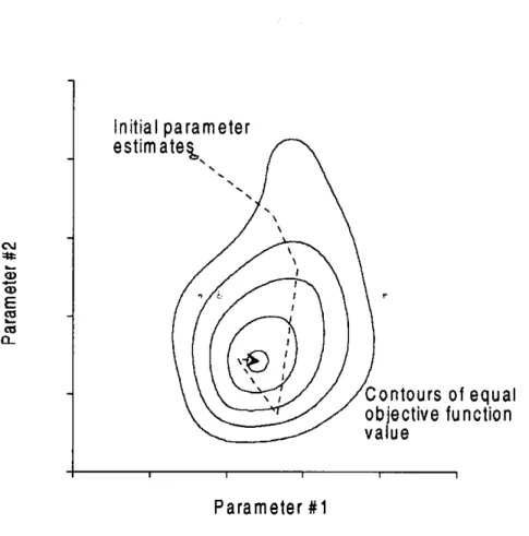
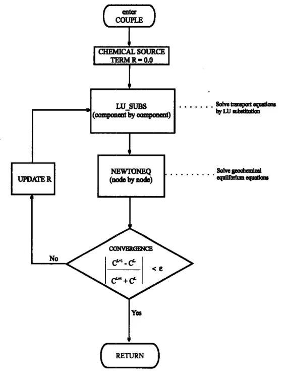
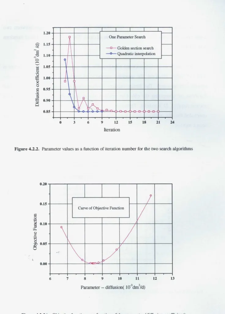
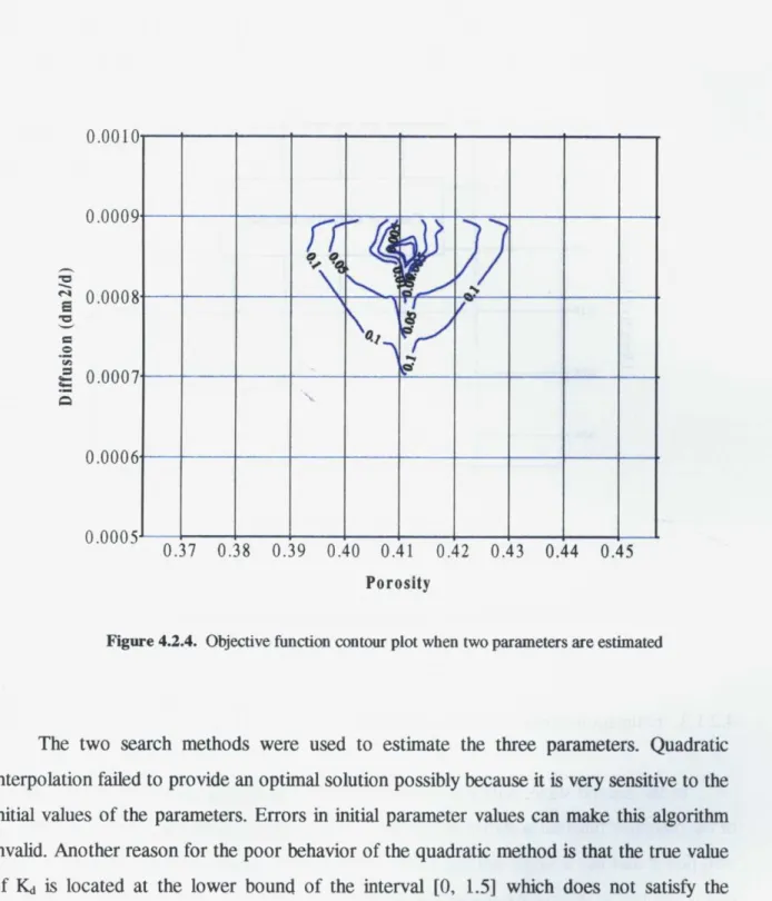
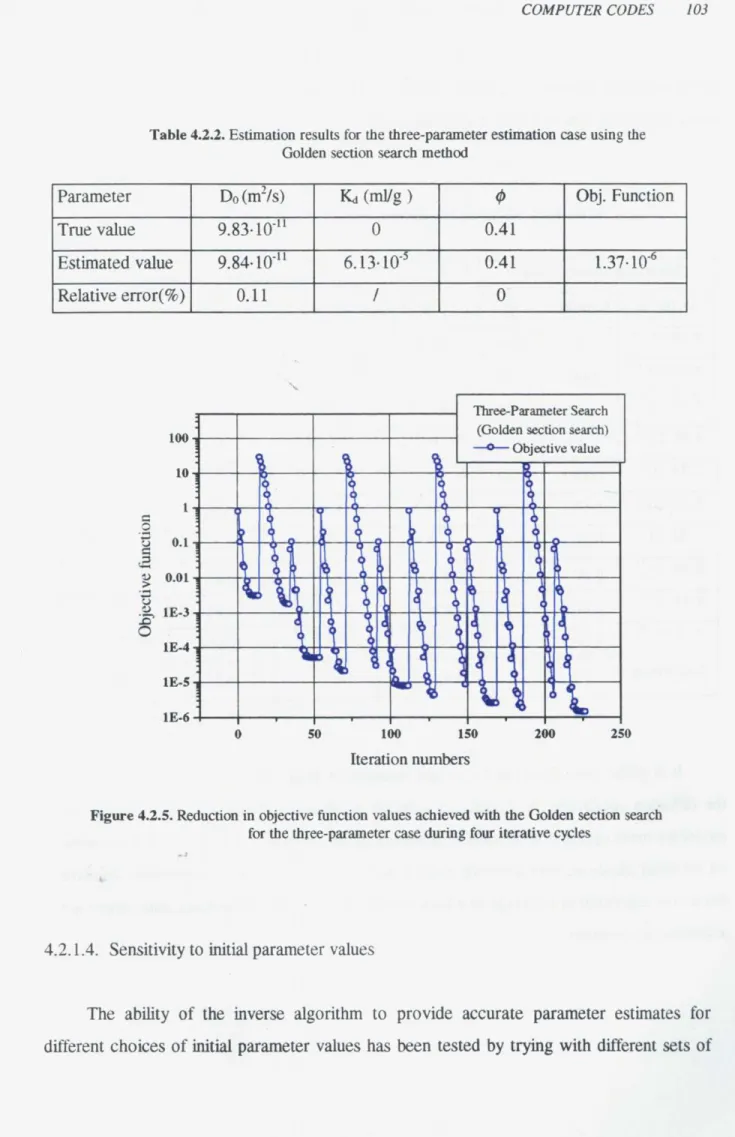
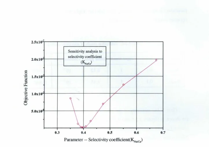
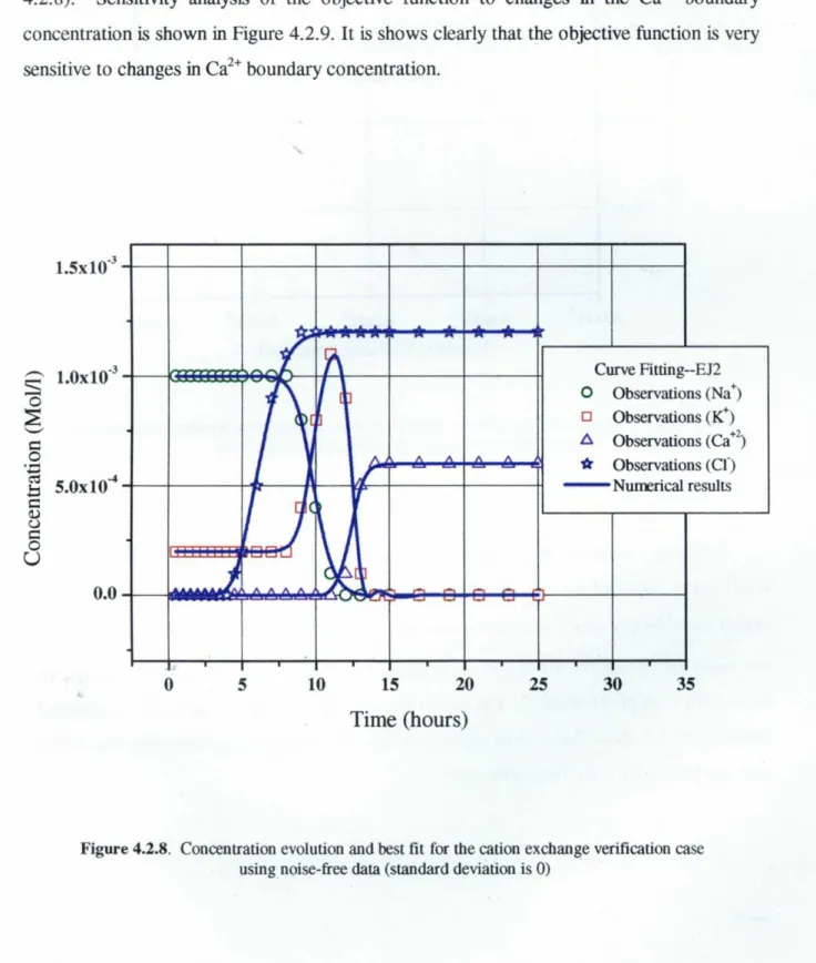
(26) INVERSE PROBLEM OF REACTNE SOLUTE TRANSPORT. ^jj. LIST OF FIGURES. Figure 3.3.1. Objective function contour values and iterative improvement from initial parameter values towards a global minimum ........................................ 75 Figure 4.1.1. Flowchart of the INVERSE-CORE2D main program ............................ 90 Figure 4.1.2. Flowchart of the subroutine TRANQIN ............................................... 92 Figure 4.1.3.. Flowchart of the HH_FLOW subroutine which solves the groundwater. flow equation ....................................................................................... 93 Figure 4.1.4. Flowchart of the HH_HEAT subroutine which solves the heat transport equation ...........................................................:.................................. 94 Figure 4.1.5. Flowchart of the subroutine COUPLE which performs the sequential iterative process for solving reactive solute transport ........................... 95 Figure 4.1.6. Flowchart of the NEWTONEQ subroutine which solves the chemical equilibrium equations by a Newton-Raphson method ........................... 96 Figure 4.2.1. Objective function values as a function of iteration number for the two search algorithms ................................................................................ 99 Figure 4.2.2. Parameter values as a function of iteration number for the two search algorithms ......................................................................................... 100 Figure 4.2.3. The objective function as a function of the parameters ....................... 100 Figure 4.2.4. Objective function contour plot when two parameters are estimated .. 102 Figure 4.2.5. Reduction in objective function values achieved with the Golden section search for three-parameter case during four iterative cycles ................ 103 Figure 4.2.6. Sensitivity of the objective function to changes in the selectivity coefficient KN^ ................................................................................ 107 Figure 4.2.7.. Sensitivity of the objective function to changes in the selectivity coefficient Krr^ca ............................................................................... 108. Figure 4.2.8. Concentration evolution and best fit for the cation exchange verification case using noise-free data ................................................................. 111.

(27) TABLE OF CONTENTS. ^jjj. Figure 4.2.9. Sensitivity of the objective function to changes in calcium boundary concentration (Ca2+) for the case of noise-free data ............................. 112 Figure 4.2.10. Relative error of parameter estimation versus standard deviations of measurement error without parameter prior information .......................................................................................................... 113 Figure 4.2.11. Optimum value of objective function versus standard deviations of observation data ................................................................................ 114 Figure 4.2.12. Reduction of objective function with the iteration number for different conditions .......................................................................................... 115 Figure 4.2.13. Estimates of specific surface (A) and kinetic rate constant (Rk) showing a negative correlation ............................................................................ 120 Figure 4.2.14. Relative error of parameter estimation versus standard deviations of measurement error with parameter prior information ......................... 122 Figure 4.2.15. Optimum value of objective function versus standard deviations of observation data ..........:..................................................................... 123 Figure 5. l. l.. Measured cumulative water inflow and best fitt obtained with different relative permeability functions in tests SAT l, SAT2, SAT3, SAT4. and SATS ......................................................................................... 131 Figure 5.1.2.. Measured final water content distribution and best curve fit obtained with different relative permeability functions in tests SATI, SAT2, SAT3, SAT4 and SATS ................................................................................ 133. Figure 5.1.3.. Estimated relative permeability functions for tests SATI, SAT2, SAT3, SAT4 and SATS .................................................................................136. Figure 5.1.4. Measured and computed retention curves for tests SAT4 and SATS... 137 Figure 5.1.5. Plot of the Cl- concentration computed with different relative permeability functions in Test SATS ...................................................................... 139 Figure 5.1.6. Plot of the I^ concentration computed with different relative permeability functions in Test SATS ...................................................................... 139 Figure 5.2.1.. Methods used for determining sorption and diffusion parameters ....... 141. Figure 5.2.2. Activity evolution and best fit of IN and OUT reservoirs of throughdiffusion experiment TD-1 ................................................................. 146.

(28) INVERSE PROBLEM 4F REACTNE SOLUTE TRANSPORT. ^jy. Figure 5.2.3. Activity evolution and best fit of IN and OUT reservoirs of throughdiffusion experiment TD-2 ................................................................ 147 Figure 5.2.4. Activity evolution and best fit of IN and OUT reservoirs of throughdiffusion experiment TD-3 ................................................................. 147 Figure 5.2.5. Sensitivity analysis of the objective function to porosity ..................... 148 Figure 5.2.6. Sensitivity analysis of the objective function to effective diffusion coefficient ......................................................................................... 148 Figure 5.2.7. Evolution of the objective function for the two search algorithms in the interpretation of through-diffusion experiment TD-2 ......................... 150 Figure 5.2.8. Evolution of parameter values for the two search algorithms in the interpretation of through-diffusion experiment TD-2 ......................... 150 Figure 5.2.9. Activity evolution and best fit of IN and OUT reservoirs of the throughdiffusion experiments TD-SrS, TD-Sr6, TD-Sr7 and TD-Sr8 .............. 153. Figure 5.2.10. Linear relationship of the estimates of effective diffusion coefficient and Kd in strontium through-diffusion experiment TD-Sr5 ....................... 156 Figure 5.2.11. Measured data for experiments of ID-Cs-9 (left) and ID-Cs-10 (right) 161 Figure 5.2.12. Best fit of activities in cla.y plug (left) and in reservoir of ID-Cs-9....... 163 Figure 5.2.13. Best fit of activities in clay plug (left) and in reservoir (right) of ID-Cs- l0A .........................................................................................163 Figure 5.2.14. Best fit of activities in clay plug (left) and in reservoir (right) of ID-Cs- lOB ........................................................................................ 164 Figure 5.2.15. Best fit of activities in reservoir and fmal profile activity in clay plug of ID-Se-17 ........................................................................................... 166 Figure 5.2.16. Best fit of activities in reservoir and final profile activity in clay plug of ID-Se-18 ........................................................................................... 166 Figure 5.2.17. The finite element mesh of the two-D double-porosity model ............. 168 Figure 5.2.18. Activity evolution and best fit of permeation experiment 1(P-1) ......... 169 Figure 5.2.19. Activity evolution and best fit of permeation experiment 2(P-2} ........ 170 Figure 5.2.20. Activity evolution and curve fit of permeation experiment 1(P-ld) using a double porosity model ................................................................... 174.

(29) TABLE OF CONTENTS. ^jI. Figure 5.2.21. Activity evolution and curve fit of permeation experiment 2(P-2d) using a double porosity model ..................................................................... 174 Figure 5.2.22. Time functions used to define the tracer pulse of the inflow water ...... 175 Figure 5.3.1. Best fit of HTO breakthrough curve in permeation experiment P-1G. on granite ....................................................................................... 184 Figure 5.3.2. Best fit of HTO breakthrough curve in permeation experiment P-1G on granite .......................................................................................... 184. Figure 5.4.1. Measured (symbols) and computed (lines) concentration breakthrough curves in Case 1 when only exchange reactions are considered ........... 190 Figure 5.4.2. Measured (symbols) and computed (lines) concentration breakthrough curves in Case 2 when only exchange reactions are considered ........... 193 Figure 5.4.3. Measured (symbols) and computed (lines) concentration breakthrough curves in Case 6 when only exchange reactions are considered ........... 200 Figure 5.4.4. Measured (symbols) and computed (lines) concentration breakthrough curves in Case 7 when only exchange reactions are considered ........... 204 Figure 5.4.5. Measured (symboLs) and computed (lines) concentration breakthrough curves in Case 8 ................................................................................ 209. Figure 5.5.1. Computed (lines) and Measured (symboLs) concentrations of dissolved species after 3200 years when estimating 10 parameters (Case 1) ...... 217 Figure 5.5.2. Computed (lines) and Measured (symbols) concentrations of dissolved spécies after 3200 years when estimating 10 parameters (Case 3) ...... 222. Figure 5.6.1. Outline of the Aquia aquifer in Maryland with estimated prepumping head distribution ........................................................................................ 226 Figure 5.6.2.. Schematic cross section of the Aquia aquifer ...................................... 226. Figure 5.6.3. Calcite, dolomite and magnesite saturation indexes calculated from chemical data of the Aquia aquifer using EQ3 ..................................... 229 Figure 5.6.4.. Measured (symboLs) and computed (lines) concentrations at Aquia aquifer (Case 1) ............................................................................................ 234. Figure 5.6.5.. Measured (symbols) and computed (lines) concentrations at Aquia aquifer. (Case 2} ............................................................................................ 236 Figure 5.6.6. Measured (symbols) and computed ( lines) concentrations at Aquia aquifer (Case 3) ............................................................................................ 239.

(30) INVERSE PROBLEM OF REACTIVE SOLUTE TRANSPORT. ^jlj. Figure 5.6.7. Measured (symbols) and computed (lines) concentrations at Aquia aquifer (Case 4) ............................................................................................ 242 Figure 5.6.8. Measured (square) and computed (at different times) concentrations at Aquia aquifer (Case 5) ...................................................................... 245 Figure 5.6.9. Computed exchanged cation concentrations (at different times) at Aquia aquifer (Case 5) ................................................................................. 248 Figure 5.6.10. Computed aqueous Cl- concentrations (at different times) at Aquia aquifer (Case 5) ............................................................................................ 250 Figure 5.6.11. Cal^ite dissolution (negative values) (at different times) at Aquia aquifer . (Case 5) ............................................................................................ 250.

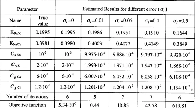
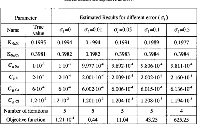
(31) TABLE OF CONTENTS. ^j/jj. LIST OF TABLES. Table 4.2.1. The prior information of the parameters ............................................... 159. Table 4.2.2. Estimation results for the three-parameter case using the Golden section search method ...................................................................................... 103 Table 4.2.3. Sensitivity of estimation results to initial parameter values ................... 104 Table 4.2.4. Initial and boundary total dissolved concentrations (moUl) ................... 106 Table 4.2.5. Estimation results of selectivity coefficients ......................................... 107 Table 4.2.6. Information of the parameters to be estimated ....................................... 109 Tabe 4.2.7. Estimation results using synthetic concentration data containing different levels of noise. No prior information about parameters is considered .... 109 Tabe 4.2.8. Estimation results using synthetic concentration data containing different degrees of noise. Parameter prior information is considered in the objective function (wp=1) ................................................................................... 110 Tabe 4.2.9. Estimation results using synthetic concentration data containing different degrees of noise. Parameter prior information is considered in the objective function (wp=10) ................................................................................. 110 Table 4.2.10. Initial and boundary total dissolved concentrations (moUl) of the components of problem EJ2KIN .......................................................... 117 Table 4.2.1 l. Information of the parameters to be estimated ...................................... 118 Tabe 4.2.12. Estimated results using synthetic concentration data with different levels of noise ( µ^ =1) without prior information (wp=0) ..................................... 119 Tabe 4.2.13. Estimated results using synthetic concentration data with different levels of noise ( µ^ =1) and considering prior parameter information (wp=1) ........................................................................................................ 121 Table 5.1.1. Summary of the infiltration experiment data .......................................... 126.

(32) INVERSE PROBLEM OF REACTNE SOLUTE TRANSPORT. ^l/jjj. Table 5.1.2. The prior information, lower and upper bounds of the parameters......... 128 Table 5.1.3. Estimation results for test SAT1 ........................................................... 129 Table 5.1.4. Estimation results for test SAT2 .......................................................... 129 Table 5.1.5. Estimation results for test SAT3 .......................................................... 129 Table 5.1.6. Estimation results for test SAT4 .......................................................... 130 Table 5.1.7. Estimation results for test SATS ...................................,....................... 130 Table 5.2.1. The prior information of the parameters of the through-diffusion experiments ....................................................................................... 144 Table 5.2.2. Estimated diffusion coefficient by different methods ............................. 144 Table 5.2.3.. Estimated diffusion coefficient and porosity by numerical methods ..... 146. Table 5.2.4. Prior information of strontium parameters ........................................... 151. Table 5.2.5. Estimates of diffusion coefficient (Do, De and Da), Kd and porosity from strontium through-diffusion experiments .............................................. 152 Table 5.2.6. Cesium diffusion coefficients estimated with the analytical method ...... 160 Table 5.2.7. Parameter prior information for cesium in-diffusion experiments ......... 161. Table 5.2.8. Estimates of diffusion coefficient (Do, De and Da), Kd and porosity from . . . . . cesium in-d. sion experunents .......................................................... 162. Table 5.2.9. Parameter prior information for selenium in-diffusion experiments ....... 165 Table 5.2.10. Estimates of diffusion coefficient (Do, De and Da), Kd and porosity from selenium in-diffusion experiments ....................................................... 165 Table 5.2.11. Prior information of the parameters of the permeation experiments ...... 168 Table 5.2.12. The estimated results of single porosity model .................................... 169 Table 5.2.13. Prior information of the parameters for double-porosity model ............ 172 Table 5.2.14. Estimated results of permeation experiments using a double porosity models ............................................................................................... 172 Table 5.2.15. Summary of interpretation of CIEMAT diffusion experiments performed on compacted FEBEX bentonite ....................................................... 180.

(33) TABLE OF CONTENTS. ^X. Table 5.3.1. Prior information and upper and lower bounds of the parameters ........ 182 Table 5.3.2. Estimation results for permeation experiments in granite samples ........ 183 Table 5.4.1. Initial and boundary total dissolved concentrations of components in Ketelmeer sediment ........................................................................... 187. Table 5.4.2. Parameter prior information data ......................................................... 189 Table 5.4.3. Estimated results for selectivity coefficients (Case 1) considering only cation exchange reactions and a fixed CEC=10.lmeq/100g ...... 189 Table 5.4.4. Estimation results for Case 2 ............................................................... 192 Table 5.4.5. List of additional chemical reactions considering in Case 3 ................... 195 Table 5.4.6. Estimation results for Case 3 .............................................................. 196 Table 5.4.7. Estimation results for Case 4 .............................................................. 197 Table 5.4.8. Estimation results for Case 5 ............................................................... 198 Table 5.4.9. Estimation results for Case 6 ............................................................... 199 Table 5.4.10. Estimation results for Case 7 ............................................................... 203 Table 5.4.11. Objective function and the contribution of each component for Cases 6, 7 and 8 ................................................................................................. 203 Table 5.4.12. Estimation results for Case 8 ............................................................... 207 Table 5.5.1. List of geochemical reactions considering for the Llobregat Delta aquitard .............................................................................................. 212 Table 5.5.2. Initial and bottom boundary total dissolved chemical component concentrations ................................................................................... 213 Table 5.5.3. Cation selectivity (Gaines-Thomas convention) and CEC values initially calculated from experimental data ........................................................213 Table 5.5.4. Measured concentrations at well CM (moUl) and the weighting coefficients for each chemical species ................................................. 214 Table 5.5.5.. Lower and upper bounds and prior parameter information for the case without redox reaction ....................................................................... 215. Table 5.5.6. Ir^ tial guess, estimated values, estimation variance and confidence intervals for the case without redox reactions ................................................. 216.

(34) INVERSE PROBLEM OF REACTNE SOLUTE TRANSPORT. ^xX. Table 5.5.7. Lower and upper bounds and prior parameter information for the case with redox reactions ................................................................................... 219 Table 5.5.8. Initial guess, estimated values, estimation variance and confidence intervals for the case with redox reactions (Case 2) ............................................ 220 Table 5.5.9. Initial guess, estimated values, estimation variance and confidence intervals for the case with redox reactions (Case 3) ............................................ 221 Table 5.6.1. Initial and boundary total dissolved concentrations in Aquia aquifer ..... 230 Table 5.6.2. Prior information data .......................................................................... 232 Table 5.6.3. Parameter estimates for Case 1 ............................................................ 233 Table 5.6.3. Estimation results of the Aquia aquifer for Case 2 ................................ 235 Table 5.6.4. Estimation results of the Aquia aquifer for Case 3 ................................ 238 Table 5.6.5. Estimation results of the Aquia aquifer for Case 4 ................................ 241 Table 5.6.6. Estimation results of the Aquia aquifer for Case 5 ................................ 244 Table A2.1. True and noise-corrupted concentration data( ^t^ =1) ............................ 286.

(35) INTRODUC7'ION. 1. CHAPTER 1. INTRODUCTION. 1.1. MOTIVATION. The assessment of the performance of waste disposal facilities requires a quantitative analysis of the migration of toxic substances away from the repository. This in turn requires the use of modeling tooLs which are able to analyze both the transport of dissolved species as well as their complex interactions with the solid phases of the engineering and geological barriers. Computer simulations based on numerical models have been increasingly used for these purposes, a trend that undoubtedly will continue as more sophisticated models aze being developed and computer costs keep decreasing. Significant efforts and attempts have been made during recent years towards the development of such tooLs.. However, with greater forward model sophistication the need comes for more accurate data requirements. The real improvement in precision will eventually hinge on our ability to determine accurately the required model parameters, such as saturated permeability, porosity, relative permeability, diffusion and dispersion coefficients, initial and boundary concentrations, initial pH and pE, selectivity coefficients for cation exchange, cation exchange capacity (CEC), the kinetic parameters such as specific surface of mineral, apparent activation energy, kinetic rate constant, the exponent of the catalytic term and the exponent of ratio of the ionic activity product and the equilibrium constants. Unfortunately, over the past 20 years, it appears that the ability to fully characterize the parameter systems of the reactive transport models has not kept pace with the numerical and modeling expertise. Difficulties in model calibration are nowhere more evident than in the analysis of flow and reactive solute transport in the unsaturated zone. There is a clear need for the development of general purpose and numerically efficient codes that can estimate.

(36) INVERSE PROBLEM OF REACTNE SOLUTE TRANSPORT 2. simultaneously some or all the relevant hydrodynamic, solute transport and hydrochemical parameters by robust optimization techniques.. 1.2. STATE-OF-THE-ART. Building a model for a groundwater flow and reactive solute transport system requires solving two problems, the forward problem (simulation) and its inverse (calibration) (Sun, 1994). The former predicts unknown system states by solving appropriate governing equations, while the latter determines unknown physical and chemical parameters and initial and boundary conditions of the system. One must first solve the inverse problem to find appropriate model structure and model parameters, and then solve the forward problem to obtain prediction results.. 1.2.1. FORWARD MODELING OF REACTIVE SOLUTE TRANSPORT. In the past decade, coupled models accounting for complex hydrological and chemical processes, with varying degrees of sophistication, have been developed. Samper et al. (1995) presented a state-of-the-art on hydrogeochemical, water flow and reactive solute transport models. Existing models of reactive transport employ two basic sets of equations: the transport equation and chemical equation. Two major numerical approaches have been proposed to solve the coupled problem (Yeh and Tripathi, 1989; Xu et al, 1999): (1) Direct substitution approach (DSA) according to which chemical equations are directly substituted into the transport equations and (2) sequential iteration approach (SIA) in which transport and chemical equations are solved separately in a sequential manner and following an iterative procedure. DSA leads to a system of coupled highly non-linear transport equations. It was used by Carnahan (1990), Steefel and Lasaga (1994), White (1995), Ayora et al. (1998), Saaltink et al. (1998) and Saaltink (1999). Its main advantage is high accuracy and quadratic rate of convergence. Especially for chemically difficult (that is, highly non linear) cases, when the SIA requires very small time steps leading to excessive computation times, the DSA is consistently very robust and does not show this inconvenience (Saaltink, 1999)..

(37) INTRODUCTION. 3. However, For chemically simple cases but with grids of many nodes, the SDA tends to be less favorable because of the size of the set of equations to be solved. It is very demanding in terms of computing time and memory. This can seriously limit its use for large problems (Yeh and Tripathi, 1989). On the contrary, the sets of equations that are solved simultaneously in the SIA are much smaller than in the DSA, and therefor, larger systems with larger sets of chemical species can be handled with SIA. This approach was used by many investigators, such as Liu and Narasimhan (1989), Nienhuis et al (1991), Yeh and Tripathi (1991), Delgado et al. (1999), Engesgaard and Kipp (1992), Samper and Ayora (1994), Samper et aL (1998), Samper et al. (1999 a, b), Lensing et al. (1994), Simunek and Suarez (1994), Walter et al. (1994a, b), Zysset et aL (1994a, b), Neretnieks et aL (1997), and Xu et al. (1999).. A mixed model containing ion exchange and surface complexation is included in the PHREEQM code (Appelo and Postma, 1993). It consists of a one-dimensional transport code coupled to the PHREEQE (Parkhurst et aL, 1980) geochemical code. The solution of the advection-dispersion equation is based on the mixing cell concept. For each time step and for each cell, the modified PHREEQE version computes aqueous speciation and mass transfer to/from mineraLs. Ion exchange reactions are incorporated into the PHREEQE database as half reactions of the cations with a fictitious species representing the sorbent substrate. The thermodynamic activities of sorbed species are calculated from equivalent fractions following the Gaines-Thomas convention. PHREEQM allows also calculating H+ adsorption/desorption following a surface complexation model with the electrostatic term computed from a constant capacitance modeL PHREEQM has been successfully applied to the description of the zonation of the chemical composition of groundwater in saline intrusion processes and refreshening of saline aquifers (Appelo, 1994).. Walter et aL ( 1994) presented the. code which consists on coupling the finite. element transport model PLiJME2D and MINTEQA2 equilibrium geochemistry modeL These authors claim that making use of the local equilibrium assumption, the inherent nonlinearity is confined to the chemical domain. This linearizes the coupling between physical and chemical processes and leads to a simple and efficient two-step sequential solution algorithm (without iteration). The program can handle realistic aquifer properties and boundary conditions. The..

(38) INVERSE PROBLEM OF REACTNE SOLUTE TRANSPORT 4. geochemical equilibrium model MINTEQA2 includes aqueous complexation, acid-base reactions, oxidation-reduction by either fixing the solution pE value or using the activities of electroactive species, cation exchange by constant charge model, adsorption via surface complexation by the constant capacitance, the diffuse layer and the triple-layer models. Adsorption isotherm models (Kd approach) are also included in the modeL Activity coefficients are calculated using the extended Debye-Hiickel and Davies equations. The Newton-Rapson iterative technique is used for solving the chemical equations.. Version 2 of _ PHREEQC (Parkhurst, 1999) is a computer program written in C that is designed to perform a wide variety of low-temperature aqueous geochemical calculations. It is based on an ion-association aqueous model and has capabilities for: (1) speciation and saturation-index calculations, (2) batch-reaction and one-dimensional (1 D) transport calculations involving reversible reactions, which include aqueous, mineral, gas, solidsolution, surface-complexation, and ion-exchange equilibria, and irreversible reactions, which include specified mole transfers of reactants, kinetically controlled reactions, mixing of solutions, and temperature changes, and (3) inverse modeling, which finds sets of mineral and gas mole transfers that account for differences in composition between waters, within specified compositional uncertainty limits.. Additional features in version 2 of PHREEQC. relative to version 1(Parkhurst, 1995) include capabilities to: (1) simulate dispersion (or diffusion) and stagnant zones in 1D-transport calculations, (2) model kinetic reactions with user-defined rate expressions,. (3) model the formation or dissolution of ideal,. multicomponent or nonideal, binary solid solutions, fixed-volume gas phases in addition to fixed-pressure gas phases, (4) allow the number of surface or exchange sites to vary with the dissolution or precipitation of minerals or kinetic reactants, (5) include isotope mole balances in inverse modeling calculations, and (6) automatically use multiple sets of convergence parameters. However, the capacities of this model to simulate flow and solute transport are limited.. Samper et al. (1999) developed a 2-D fu^te element multi-components reactive transport code, CORE2D, (a COde for modeling water flow saturated or unsaturated, heat transport and multicomponent REactive solute transport under local chemical equilibrium or kinetic conditions), which can use either SIA or SNIA (Sequential non-iterative approach).

(39) IN7RODUCTION. 5. for the purpose of improving numerical efficiency. General water flow, heat transfer and solute transport boundary conditions are considered under fully or variably saturated media. The code accounts for a wide range of chemical processes such as aqueous complexation, acid-base, redox, mineral dissolution/precipitation (kinetic), gas dissolution/ exsolution, cation exchange, and adsorption via surface complexation. This code has been widely used in several research projects dealing with radioactive waste disposal at laboratory and field scales (Samper et al., 1998, 1999 and Delgado et aL, 1999).. 1.2.2. INVERSE MODELING OF REACTIVE SOLUTE TRANSPORT. As a whole, the solution of the inverse problem is still limited to flow and conservative solute transport models. In most of case studies, very fine reactive transport models are usually calibrated by trial-and-error method. Sophisticated inverse models are only available for estimating flow and solute transport parameters. A considerable effort has been devoted to estimation of flow parameters, and the number of studies of the groundwater flow inverse problem is large. Several different methods have been applied. Field-scale applications are also numerous (Neuman et al., 1980; Cooley, 1983; Carrera and Neuman, 1986c). Comprehensive reviews of the inverse problem of aquifer flow are provided by Yeh (1986), Carrera (1987), Sun (1994) and Samper and García-Vera (1998).. 1.2.2.1. Inverse analysis of flow in variably saturated media. Over the past 15 years, interest has arisen in the feasibility of using inverse algorithms to analyze soil hydraulic properties from transient infiltration events (Kool et al., 1985; Parker et al., 1985; Kool and Parker, 1988; Russo, 1988; Yeh and Harvey, 1990; Russo et al., 1991; Kabala and Milly; 1991; Zayani et al. 1991; Eching et aL, 1994). MorelSeytoux et al. (1996) studied the parameter equivalence for the Brooks-Corey and van Genuchten soil characteristics and provided a simple way for the conversion between these two sets of parameters. Simunek and van Genuchten (1996) estimated the hydraulic properties of unsaturated soiLs via numerical inversion using a tension disc infiltrometer..

(40) INVERSE PROBLEM OF REACTNE SOLUTE TRANSPORT 6. Inoue et al. (1998) demonstrated the potential application of the soil water extraction method for estimating soil water retention and unsaturated hydraulic conductivity parameters in the field. The method of simulated annealing is a technique that has attracted significant attention as suitable for optimization problems, especially for problems in which a desired global extremum is hidden among many, poorer, local extrema (Press et al, 1992). Pan and Wu (1998) developed a hybrid global optimization method which incorporates simulated annealing strategies into a classical downhill simplex method. They used the annealing-simplex method for the estimation of hydraulic parameters. The computing efficiency of this method, however, is greatly limited by the number of parameters.. 1.2.2.2. Coupled inverse modeling of flow and solute transport. The coupled inverse approach provides a way whereby measurements of state are used to determine unknown flow and transport parameters by fitting the model output with the measurements. Wagner and Gorelic (1987) considered optimal groundwater quality management under parameter uncertainty in which a coupled flow-mass transport model was identified, and the parameter uncertainty was estimated. Chu et al. (1987} discussed data requirements for the calibration of a flow-mass transport model to determine unknown transmissivities and dispersivities. Woodbury et al. (1987) and Woodbury and Smith (1988) used temperature measurements to improve the estimation of hydraulic conductivities, in which a coupled inverse problem of flow and heat transport was solved. Kool and Parker (1987) and Mishra and Parker (1989) considered the inverse problem for coupled unsaturated flow and mass transport. A general framework and description of the coupled inverse problems of flow and transport is given by Sun and Yeh (1990). They defined the objective function based on an L2 norm for each problem and coupled them with weighting coefficients to form a scalar objective function and the Jacobian matrix was computed by the adjoint state method. Samper et al. (1990), used an automatic calibration technique to construct a groundwater flow and solute transport model for the quantitative assessment of groundwater uranium pollution from a mill tailings pond in Southern Spain. They also performed sensitivity and uncertainty analyses related to flow and solute transport parameters. Gailey et al. (1991) demonstrated a field application of the model presented by.