A Note on the Need to Account for Spatial Dependence: A Case of Migratory Flows in Spain

(1)

The Review of Regional Studies 2008, Vol. 38, No. 1, pp. 105–111

© Southern Regional Science Association 2010. ISSN 1553-0892

SRSA, 1601 University Avenue, PO Box 6025, Morgantown, West Virginia 26506-6025, USA.

A Note on the Need to Account for Spatial Dependence: A Case of Migratory

Flows in Spain

Adolfo Maza and José Villaverde

ABSTRACT: The potential existence of spatial dependence in the relevant literature on migratory flows has not been dealt with sufficiently. This paper tries to fill this gap by applying spatial statistic techniques to the Spanish case. First, the paper shows that there is indeed spatial dependence in some of the variables conventionally included in migration equations. Second, these variables are filtered to remove spatial dependence. Third, in order to evaluate the influence of spatial dependence on migration, a conventional migration equation is estimated with both actual and filtered data, revealing key differences. Spatial dependence clearly matters in migration analysis.

Key Words: migratory flows; spatial dependence; spatial filtering, Spanish provinces. JEL Classification: J61; R23; C21

1. INTRODUCTION

Migratory flows are pervasive in economic history. Generally speaking, people migrate to improve their quality of life. It is a process that, from an economic perspective, tends to equilibrate spatial differences in terms of both per capita income and unemployment rates.

Although the migration literature offers many interesting insights on the topic, there are at least two methodological issues that have not been dealt with sufficiently: on the one hand, most of the migration studies seem to “ignore the problem of finding the best functional form for the migration model” (Cushing and Poot, 2004, p. 324); on the other, spatial features of migratory flows have received relatively scant attention.1 As a way to try to overcome the first issue, Maza and Villaverde (2004) apply a semiparametric approach to explain the internal migratory flows in Spain in terms of a conventional migration model. As for the second issue, it has been proved that the presence of spatial effects between certain economic areas may lead to inconsistent results in standard regression equations (Anselin, 1988). But, as Cushing and Poot (2004, p. 318) indicate, “rapid developments in spatial econometrics have not yet found much application in migration research.” By using the Spanish provinces for the period 1996 to 2003 as a “laboratory,” the aim of this note is to begin to fill this gap. In order to do that, we extend the model presented in Maza and Villaverde (2004) by examining spatial dependence.2 More



Maza and Villaverde are affiliated with the Department of Economics, University of Cantabria. They thank the editors and two anonymous referees for their useful comments and suggestions. The usual disclaimer applies.

Contact author: Adolfo Maza, University of Cantabria, Department of Economics, Avda. de los Castros, s/n, 39005-Santander

(Spain), Telephone: +34-942-201652; Fax: +34-942-201603. E-mail: mazaaj@unican.es.

1

Among the papers that have dealt with this issue, see, for example, Aroca, Hewings, and Godoy (2001), Lundberg (2003), Rupasingha and Goetz (2004), Rovolis and Tragaki (2005), Soloaga and Lara (2005), Basile and Causi (2006), and LeSage and Pace (2008).

2

(2)

precisely, we apply a spatial filtering technique that to the best of our knowledge has not been employed before in the migration literature.

2. A SPATIAL ANALYSIS APPROACH TO MIGRATION

Drawing from Maza and Villaverde (2004), an extended gross migration equation for province i in period t is:

(1) it it it it it it it it it it i it agr d s cl h k pr y u gmr                                 1 9 1 8 1 7 1 6 1 5 1 4 1 3 1 2 1 1 _,

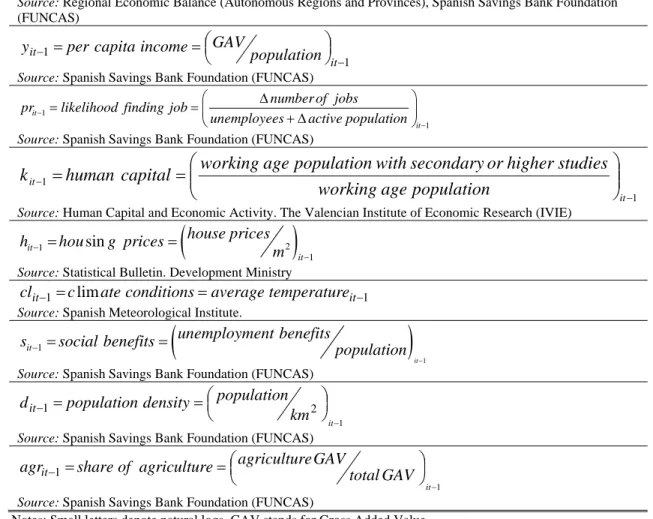
where the definitions of the variables as well as the sources from which they have been extracted are shown in Table 1.3

Usually, an equation like the previous one is estimated by employing actual, untransformed data. Nonetheless, some variables included in Equation (1) might be affected by spatial dependence (albeit for different reasons like similarities in production structures or demographics, spillover effects, etc.). By “spatial dependence” we typically mean the geographic coincidence of value similarity. If it exists, econometric problems can result: in particular, the estimates could be biased and inconsistent.4

Then, in order to test for the existence of spatial dependence in the aforementioned variables, we compute Moran’s I statistic:

(2)













, , 2 i j i j i j i j i i j i w x x x x n I w _x _x    



_

,

where x xi

 

j is the variable under consideration for province i

 

j , xis the average value of this

variable across provinces, and w is an element of the distance matrix i j,

 

W between each pair of

provinces.5 To calculate this statistic, we have used the inverse of the standardized distances between each origin and destination as the distance matrix.

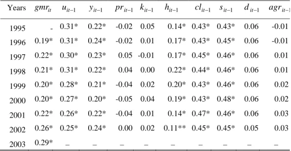
The results obtained by applying Equation (2) are displayed in Table 2. These results show that variables such as gross migration rates, unemployment rates, housing prices, climate and social benefits are spatially dependent. Remaining variables show no signs of spatial autocorrelation.

3

The new model employs gross rather than net migration flows since net migration flows could mask the presence of much larger gross flows. In addition, it is convenient to note that, as it is stated by the definition of the dependent variable, this model does not consider the destination province.

4

Although the aim of this paper is to consider spatial dependence problems, it is worth mentioning that there are other “more traditional” econometric problems that could lead to biased and/or inconsistent results in Equation (1), such as heteroskedasticity, autocorrelation, endogeneity, etc.

5_{In order to compute the significance level of Moran’s I statistic we have assumed that the standardized statistic follows a normal}

distribution; for the sake of robustness, we have also used two other approaches (the randomization and permutation approaches) and the results are roughly the same.

(3)

MAZA &VILLAVERDE:NOTE ON THE NEED TO ACCOUNT FOR SPATIAL DEPENDENCE 107

TABLE 1. Definition and Sources of Variables 1000 1           it it

it grossmigrationrate migrants _population

gmr

Source: Statistics of Residential Variations. Spanish National Statistics Institute (INE)

1

it

u _ rate of unemployment

Source: Regional Economic Balance (Autonomous Regions and Provinces), Spanish Savings Bank Foundation

(FUNCAS) 1 1    _ _ it it percapitaincome GAV _population

y

Source: Spanish Savings Bank Foundation (FUNCAS)

1

it

number of jobs pr likelihood finding job

unemployees active population       _{ } _    

1 1           it it population age working studies higher or secondary with population age working capital human k

Source: Human Capital and Economic Activity. The Valencian Institute of Economic Research (IVIE)



2



1 1 sin it it house prices h hou g prices m    

Source: Statistical Bulletin. Development Ministry

1

1 lim 

   it

it c ateconditions averagetemperature

cl

Source: Spanish Meteorological Institute.





1 1 it it unemployment benefits

s social benefits _population



  

1 2 1           it km population density population d_it

1 1           it GAV total GAV e agricultur e agricultur of share agr_it

Notes: Small letters denote natural logs. GAV stands for Gross Added Value.

After having proved the existence of spatial dependence, some explanations, either by modeling or filtering, need to be given. Spatial modeling (through spatial lag, spatial error and spatial autoregressive SAR models) is a powerful method. One spatial modeling approach is spatial filtering. Here the main idea is “to separate the regional interdependencies by partitioning the original variable into two parts—a filtered nonspatial (so-called ‘spaceless’) variable and a residual spatial variable—and use conventional statistics techniques…for the filtered (‘spaceless’) variables” (Gumprecht, 2005, p. 4). Although both approaches usually yield similar results, the main advantage of the spatial filtering approach is its simplicity.6

Accordingly, we opt to filter our spatial dependence variables. The filtering method we use is that proposed by Getis (1995). It is designed to convert spatially dependent variables, x,

into spatially independent variables, xf, as follows:

6

(4)

TABLE 2. Spatial Dependence in Provincial Variables Included in Equation (1)

Years gmr_it u_it_₁ y_it_₁ pr_it_₁ k_it_₁ h_it_₁ cl_it_₁ s_it_₁ d_it_₁ agr_it_₁ 1995 - 0.31* 0.22* -0.02 0.05 0.14* 0.43* 0.43* 0.06 -0.01 1996 0.19* 0.31* 0.24* -0.02 0.01 0.17* 0.43* 0.45* 0.06 -0.01 1997 0.22* 0.30* 0.23* 0.05 -0.01 0.17* 0.45* 0.46* 0.06 0.01 1998 0.21* 0.31* 0.22* 0.04 0.00 0.22* 0.44* 0.46* 0.06 0.01 1999 0.20* 0.28* 0.21* -0.04 0.02 0.20* 0.43* 0.46* 0.06 0.02 2000 0.20* 0.27* 0.20* -0.05 0.04 0.19* 0.43* 0.48* 0.06 0.02 2001 0.22* 0.26* 0.22* -0.04 0.01 0.14* 0.47* 0.46* 0.06 0.03 2002 0.26* 0.25* 0.24* 0.00 0.02 0.11** 0.45* 0.45* 0.05 0.03 2003 0.29* – – – – – – – – –

Notes: Figures represent Moran’s I statistic; * = Significant at 99%; ** = Significant at the 95%.

Sources: INE, FUNCAS, IVIE, Development Ministry, Spanish Meteorological Institute and own elaboration.

(3)

 



  

  i j ij i f i G N w x x 1    , with: (4)

 

, ij j j i j j w x G i j x   







where  is a distance parameter indicating the extent to which further distant observations are down-weighted. To apply this filter, the inverse of the standardized distance is also used as a distance matrix. Therefore, we assume the function w_ij

 

 d_ij, where  1 and d the is the _ij

distance between provincial capitals i and j.

It is worth mentioning that, besides the filtering approach used in this paper, the literature considers alternative spatial filtering schemes. Among them, the Griffith approach, based on an Eigen function decomposition associated with Moran’s I statistic of spatial autocorrelation, is

one of the most commonly employed (Griffith, 1996).7 Although this approach is also suitable for our purposes, we employ the Getis filtering method as it has been shown to be effective (Getis and Griffith, 2002), yet computationally simpler.

Subsequently, in order to evaluate the influence of spatial dependence on migration, we estimate Equation (1) by two-step feasible generalized least squares (FGLS), with actual and filtered data. FGLS estimation extends the traditional ordinary least squares (OLS) technique to a more

7

(5)

general problem than that where residuals have constant mean, a constant variance, and are uncorrelated. We have opted for FGLS estimation here because residuals obtained in the OLS estimation of Equation (1) are heteroskedastic and serially autocorrelated.8

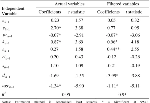
A rapid glance at the first two columns of Table 3 (actual variables) reveals the following. First, and contrary to what theory predicts, high per capita income levels in the home province are, apparently, not a factor of attraction but of population repulsion; this suggests that a model of compensating differentials is at work in the Spanish case. Second, human capital is clearly and positively related to migration rates. Third, a higher likelihood of finding a job discourages migration. Fourth, people living in provinces where the share of agriculture is high tend to have a lower propensity of moving than do people in provinces with a lower share. Remaining variables do not appear to have any effect on migration.

When we control for spatial dependence (see the last two columns of Table 3), some key differences crop up. This emphasizes the importance of properly dealing with spatial dependence. Specifically, per capita income becomes statistically insignificant, casting doubt on the explanatory capacity of a compensating differentials model for Spain. On the other hand, housing prices and population density become statistically significant; in particular, it so happens that high housing prices encourage migration, whereas high population density has the opposite

TABLE 3. Determinants of Migration: Standard Equation with Actual and Spatially Filtered Variables

Independent Variable

Actual variables Filtered variables Coefficients t statistic Coefficients t statistic 1  it u 0.23 1.57 0.05 0.32 1  it y 2.70* 3.38 0.77 0.95 1  it pr -0.07* -2.91 -0.07* -3.06 1  it k 0.87* 3.69 0.96* 4.18 1  it h 0.27 1.58 0.44** 2.55 1  it cl 0.20 0.43 -0.12 -0.26 1  it s 1.10 1.09 -0.21 -0.19 1  it d -1.69 -1.55 -3.99* -3.88 1  it agr -1.34* -5.90 -1.11* -5.11 R2 0.95 0.95

Notes: Estimation method is generalized least squares. * = Significant at 99%; ** = Significant at 95%; and fixed effects are not shown in the table but are available upon request. Sources: INE, FUNCAS, IVIE, Development Ministry, Spanish Meteorological Institute and own elaboration.

8

A revision of the FGLS estimation process, based on a consistent estimator of the variance function, can be seen, for example, in Greene (2000).

(6)

effect. As for the other variables, the results do not greatly change, regardless of the kind of data employed in the estimation. It is important to note, however, that the coefficient for human capital is larger than when spatial dependence is not taken into consideration.

3. CONCLUSIONS

Although spatial dependence in omnipresent, it has largely been ignored in the analysis of migratory flows. In this paper, we showed such misspecification can lead to misleading conclusions. We began by examining the presence of spatial dependence in the variables included in our migration equation. Having shown that some of the variables present clear signs of spatial dependence, we filtered them to eliminate such dependence. We then estimated the migration equation both with actual and filtered data, and observed some statistically significant differences. In view of this, we concluded that spatial dependence does indeed matter in the analysis of migratory flows.

A further feature of our findings is the relatively weak effect of many economic variables on migration flows in Spain. Indeed, our findings reveal that the two traditional economic variables normally included in models of migration, unemployment rates, and per capita income, apparently do not exert any influence on Spain’s gross migration rates. Another important conclusion is the importance of variables such as human capital, population density, and housing prices in explaining migration flows in Spain. With respect to housing prices, for example, it seems quite clear that the higher housing prices in large cities have forced many families to resettle in more affordable residential areas. This is an important cause of relocation of population towards suburban and ex-urban areas and is certainly in tune with the overwhelming volume of residential movements in Spain recently.

Finally, and from a political point of view, it is worth noting that the empirical evidence presented in this paper raises at least two potentially useful implications for Spanish policy-makers. On the one hand, it seems that a more active role in the housing market of the provincial, regional, and national administrations could help to redirect migrant flows. On the other hand, since our results reveal that human capital heavily influences migration propensities, this should encourage policy-makers to focus their attention on initiatives aimed at curtailing the so-called “brain drain,” especially in the more backward provinces.

REFERENCES

Anselin, Luc. (1988) Spatial Econometrics: Methods and Models. Kluwer: Dordrecht.

Aroca, Patricio, Geoffrey J. D. Hewings, and Jimmy Paredes Godoy. (2001) “Migración interregional y el Mercado laboral en Chile: 1977-82 y 1987-92,” Cuadernos de Economía, 38, 321–345.

Basile, Roberto and Marco Causi. (2006) “Determinants of Interregional Migration in Italy: 1991-2000,” working paper REAL 06-T-8.

Cushing, Brian and Jacques Poot. (2004) “Crossing Boundaries and Borders: Regional Science Advances in Migration Modelling,” Papers in Regional Science, 83, 317–338.

Getis, Arthur. (1995) “Spatial Filtering in a Regression Framework: Examples Using Data on Urban Crime, Regional Inequality and Government Expenditures,” in Luc Anselin and

(7)

Raymond Florax, eds., New Directions in Spatial Econometrics. Springer-Verlag: Berlín,

pp. 172–188.

Getis, Arthur and Daniel A. Griffith. (2002) “Comparative Spatial Filtering in Regression Analysis,” Geographical Analysis, 34, 130–140.

Greene, William F. (2000) Econometric Analysis. Macmillan: New York

Griffith, Daniel A. (1996) “Spatial Autocorrelation and Eigenfunctions of the Geographic Weights Matrix Accompanying Geo-referenced Data,” Canadian Geographer, 40,

351–367.

_____. (2003) Spatial Autocorrelation and Spatial Filtering. Springer: Berlin.

Gumprecht, Daniela. (2005) “Spatial Methods in Econometrics: An Application to R&D Spillovers,” Wirtschaftsuniversität Wien Research Report Series 26, Department of

Statistics and Mathematics, December.

Haining, Robert. (1991) “Bivariate Correlation and Spatial Data,” Geographical Analysis, 23,

210–227.

LeSage, James P. and R. Kelley Pace. (2008) “Spatial Econometric Modeling of Origin-Destination Flows,” Journal of Regional Science, 48, 941–967.

Lundberg, Johan. (2003) “On the Determinants of Average Income Growth and Net Migration at the Municipal Level in Sweden,” Review of Regional Studies, 33, 229–253.

Maza, Adolfo and José Villaverde. (2004) “Interregional Migration in Spain: A Semiparametric Analysis,” Review of Regional Studies, 34, 37–52.

Rovolis, Antonis and Alexandra Tragaki. (2005) “Ethnic Characteristics and Geographical Distribution of Immigrants in Greece,” European Urban and Regional Studies, 13, 99–

111.

Rupasingha, Anil and Stephan J. Goetz. (2004) “County Amenities and Net Migration,”

Agricultural and Resource Economics Review, 33, 245–254.

Soloaga, Isadoro and Gabriel Lara. (2005) “The Determinants of Migration in Mexico: Gravity and Spatial Econometric Approaches,” paper presented in the VIII Meetings of the LACEA/IADB/WB, Research Network on Inequality and Poverty, July 9.

Tiefelsdorf, M. and Daniel A. Griffith. (2007) “Semi-parametric Filtering of Spatial Autocorrelation: The Eigenvector Approach,” Environment and Planning A, 39, 1193–