STRUCTURAL DAMAGE IDENTIFICATION USING DYNAMIC
NUMERICAL MODELS
A. Samartin, P. Tabuenca,J.Garcia-Palacios
Escuela Tecnica Superior de Ingenieros de Caminos, Canales y Puerlos. VPM. Pro! Aranguren sn. 28040 Madrid, Espana. Escuela Superior de la Marina Civil. Plaza de Gamazo.
vc.
Sanlander, Es-panaavelino@mecanica.upm.es, labuencp@unican.es, jgpalacios@caminos.upm.es
Summary
In this paper a review of two main groups of structural damage identification methods by dynamic tests is presented. The first group is concerned with metallic thin structures damages or imperfections and the second one with reinforced concrete beam structures damages.
I. The first group is addressed to the detection of potential imperfections, fissures and cracks appear-ing in industrial machines, aeronautical structures and motor engines. They are typically metallic structures and the tests are carried under controlled environment conditions, such as in a labora-tory. The application of body waves, and more often, guided waves, as Rayleigh and Lamb waves, as dynamic excitation in order to detect the damage, is described.
The studied imperfections have been divided into three classes.
• Cracks, related to the structural safety. They are penetrating a significant part of the plate thickness.
• The second class of imperfections are small cracks or fissures, and they can be called par-tially penetrating ones because they are extended only to a small part of the plate thickness. Imperfections of this class are difficult to detect, because sometimes they can not be observed on the plate surfaces.
• Finally, the third class of imperfections are the superficial cracks and they are more related to the durability of the structure than to its safety. These imperfections are more connected to structural protection to the environment, i.e. to protective painting and coating.
Dynamic models used to detect the first class of imperfections have been Kirchhoff or Reissner bending thin plate. The crack detection can be achieved quite accurately by comparison between the first spatial derivatives of the mode shapes of the uncracked and cracked plates. Partially penetrating and superficial cracks have been identified by application as dynamic input of Lamb and Rayleigh waves respectively. The use of these guide waves seems to be a very promising technique for imperfection detection. However, computational problems appear. They are related to the small time step and the large number of the finite elements needed in order to reach a suitable accuracy level.
2. The second part of the paper treats a different group of dynamic identification and location of damage in civil and building structures. In particular the damage in reinforced concrete beams, typically used in bridge and building structures is studied. Detection procedures in this part differ of the first ones, because the existing structure is tested in the field and reinforced concrete is rather heterogenous material in comparison to metallic material. Normally, potential cracks are detected, during the free vibrations of the structure, by estimation of the changes either of its natural frequencies, or in its mode shapes or in the measure of its dynamic flexibility. However, in general, the differences of these values between uncracked and cracked beams are small and in some cases they can not be distinguished from the inherent measurement errors occurring during the tests.
Keywords
Damage detection, metallic plate structures, reinforced concrete structures, free vibration response, Rayleigh and Lamb waves, structural health monitoring
2 Introduction
Normally, in industrialized countries relatively few new public works (bridges, dams etc) are currently built and instead maintenance of already existing constructions is needed. Then, management of public structures is an important and rapidly demanding task to be carried out by Public Administration in these countries. This management includes maintenance and control about the structural performance of constructions. Typically the actual geometric and structural characteristics of these works are not known exactly, except if they are permanently monitored, and during their service life they can be deteriorated. Therefore, it is important to estimate their actual performance and level of safety. In this way different decisions respect to their eventual repairing or their use under extraordinary circumstances etc., can be taken.
In this direction several research programs in EU are currently under way to develop methodologies aimed to estimated the deterioration level, state and expected life of the existing structures. Among these research teams it can mentioned [BW96] and [PDPS95]. Most of the techniques used are directed to find tools, usually non destructive tests based on applying dynamic excitations to the structure [WHFYO I], able to detect the existence of structural imperfections (crack, material deterioration etc.).
Two main groups of damage detection will be discussed in this paper. The first is concerned with struc-tures composed by metallic plates and that can be tested under controlled environment conditions, usu-ally in a laboratory. The technique used to identify different classes of damage varies according to the potential structural deterioration.
Three main types of imperfections in thin structures such as plates and shells will be studied:(l) body cracks or cracks that penetrate to the whole thickness of the structure, (2) superficial cracks that affect only to a very small part of the thickness and (3) partially penetrating cracks as an intermediate imper-fection between the two former ones. The first type of imperimper-fections is relevant to the structural safety and the second is more concerned with its maintenance and protection against environment attacks. The third type of imperfections appears very often in the damaged structures. In the study of the first type of imperfections the Kirchhoff theory of thin plates under dynamic loading will be applied. For the second type of imperfections superficial waves theory will be used. Among the superficial waves, Rayleigh waves, will be considered because the superficial cracks under investigation are assumed to penetrate a very small depth in comparison to the whole plate thickness. The partially penetrating cracks will be analyzed by means of Lamb waves.
The part of paper related with this type of damage detection corresponds to the first part of a joint research work named Development ofnew techniques for non-contact, non-destructive testing by ultra-sound in which several Departments of the Technical University of Madrid and the University of Vigo are involved. In this research structural dynamic excitation devices and instruments for measurement of response are developed to detect possible imperfections in different structures, either in laboratory or in situ conditions. Here, only the part of this research related to theoretical aspects needed to mathemati-cally simulate the behavior of structures under dynamic excitation is presented. With the help of these results it may be possible to identify the imperfection, i.e. its existence and also its position and geom-etry as well. This theoretical work will be divided into two phases. In the first phase the effects on the structural response of the presence of a imperfection (crack, changes of geometry or material properties, etc) is analyzed. The subsequent second phase is the inverse problem or identification problem i.e. to find the position and geometry of the imperfections from the knowledge of the response of a damaged structure. This phase will not be addressed here. Itwill be noticed in the next sections that some of the proposed techniques for damage detection avoid or at least simplify in many cases the application of methods to solve the inverse problem.
The second group of damages are related to bridges and building reinforced concrete structures. They are tested usually in the field under very noisy conditions (uncontrolled traffic, temperature etc.) and difficult access conditions. Itis clear that, the methodology used for these cases has to be totally different to the previous one.
control their vulnerability to an increasing static and dynamic traffic and use loads. As a consequence, since some years damage assessment of structures has drawn the attention from different engineering areas. Static and dynamic non-destructive field tests have extensively been used as damage identification tools, although the dynamic identification methods have attracted more extensive research.
Different methods damage detection of reinforced concrete beams by dynamic tests are currently re-ported in the literature. In essence all these methods consist in the following steps. (I) obtain the dynamic response of the uncracked structure either in the design analysis step or by a dynamic test just after the structure completion, (2) dynamic test of the cracked structure, (3) select one or several dy-namic system characteristics (DSCs), i.e. natural frequencies, modal shapes or dydy-namic flexibilities, for comparison between the responses ofthe cracked and the uncracked structures (4) develop an analytical model of the dynamic behavior of the cracked structure and(5)identify the positions and severities of the cracks from the differences between ofDSCs previously obtained. This last step of identification it is also known as inverse problem for the crack model. To solve this problem it is necessary to solve a mini-mization problem, i.e. to find the positions and depth of the cracks such that the difference, according to some norm, between the observed dynamics DSCs for the crack and uncracked structures is minimum. Several optimization algorithms are available in order to solve the minimization problem, descendent gradient, penalization, genetic simulations, neural networks etc. in the specialized numerical literature. A review ofthe current methods of structural damage detection is presented. The different DSCs used and the models aimed to simulate the free vibrations of the cracked reinforced concrete beam are emphasized. Among these different models, needed during the cracks identification step, special attention to the one presented in [CB84], that corresponds to a simplified cracked Navier-Bemoulli (N-B) beam elastic theory is discussed. An extension of this model, that includes the possibility to consider the existence of several non symmetric cracks, i.e. cracks appearing only in one of the two beam faces, is given. Therefore, it can be seen that the dynamic behavior of the cracked beam can be expressed by the behavior of a uncracked N-B beam of longitudinally variable cross section. The characteristics of this equivalent beam depend on the crack position and the crack depth. By application of the method of finite element (FE) the DSCs can be computed. Finally, using an identification procedure based on an error function between the computed and the experimental results it is possible to find the cracks positions and their severity.
The paper is organized as follows. In the first sections the three methods of damage detection of metallic structures based on body waves, Rayleigh waves and Lamb waves are reported. In the following sections a short revision of different approaches of damage detection of reinforced concrete beams is presented. Finally, in the framework of an elastic cracked N-B beam theory and based on the Hu-Washizu variational theorem a model is described and then applied to the damage detection. The paper concludes with a discussion about possible improvements to the model in order to increase the accuracy and reliability of its results.
3 Metallic plates. Penetrating cracks
As it has been shown in [SM02] the existence and position of cracks penetrating throughout the depth of a metallic plate can be obtained by low frequency dynamic tests with out-plane excitation, i.e. subjected to bending. The first derivatives, i. e. the rotations, of the shapes modes of the plate under free vibrations can be used to this end.
In order to illustrate this possibility a simple example will be considered. Let it be a square plate of sidea,thin thicknessh and simply supported along its perimeter. The dynamic behavior of this plate is described by the following initial value-boundary value problem:
'V4w =
8
2w w=--=8;t
8w
w=--=
8
y2 w=
8w
7jt=ph82w
- D 8t2' in
0:5
x:5
a,0:5
and:5
ao
.along the boundaries andTIt x = 0,x = ao
along the boundaries andTIt y= 0,y= a fo(x,y) att = 0!I(x,y) att=O
(1)
0.9 O.k
0.'
0.0
0.5
0.'
0.1
t'le~h3 fi$ur3cm'm'(.O.7.y-O.~ lon~lud--o.070711
0.1 0.: 0.3 0.4 0.5 0.(. 0.7 O.l' 0.9
ROUJCi6nOX n"uxLU'ltm~.7.y-O.5 l"ngrtud~.070711
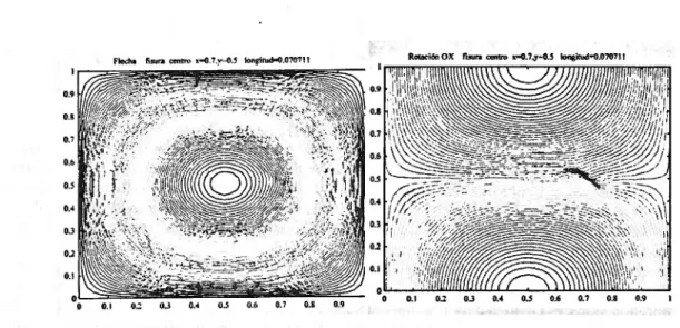
Figure 1: Modal vector1. Plate with inclined crack at(0.7a,0.5a) and length0.07a. (a) Deflectionw
isolines (b) RotationOx isolines
the plate material. The bending plate constantD is defined by the following expression:
As it is very well known the natural frequenciesWmnand the corresponding modes<I>mnare:
Wm.
~.'~
[ ( : ) \ (~)']
<I>mn= W mnsin (
n:x)
sin (n:
y)
whereWmnis a normalizing constant.
This closed form solution has been compared to a numerical solution obtained by a Finite Element (FE) method in order to calibrate the FE mesh refinement necessary to obtain the results with a given degree of accuracy. Then, the plate has been modelled by square bending Tocher-Felippa elements. A FE mesh composed by 40 x 40 elements was used and the relative error obtained for the first natural frequency was 0,05%. Similar error orders have been reachedinrelation to the vibration modal vectors ~mn = (<I>mn,i)'using different comparison norms, such as,L 2 ,standard quadratic deviation, andLoo the difference between the maximum components of normalized modal vectors.
The next step was to assume the same plate with a totally penetrating crack throughout its thickness. The crack could be placed in any point of the plate and have arbitrary length. Then the plate was identified by the following parameters: the crack centerx, y, its lengthl and inclination angle in plan or angleG respect the axisOx. Using a similar FE mesh as before a sensitivity analysis was carried out, i.e. the natural frequencies and modes of the cracked plate were obtained. In each analysis the crack was defined by different set of parameters,x,y, landG,that varies within a large range of values.
iso-ROC3to:k"'OV lisutll (<1ltre)i-o.7~-o.5 'ont:itud-O.010111
0.3 0.4 0.5 0.6 0.7 0.8 0.9 oI (J.~ 0.3 O~ 0..5 O.b U.7 O.g t1.oJ
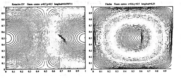
Figure 2: Modal vector 1. Plate with (a) inclined crack at (0.7a ,0.5a)and length0.07a. RotationOy
isolines (b) vertical crack at(O.Ga, 0.5a)and length 0,25a. Deflectionwisolines
O.l 1" 0.2 ' 0.1
0
0 0.1 0.2 0.1 0." O.j 0.6 0.7 0.8 0.9 0.1 0.2 0.3 0.. O.S 0.6 0.7 0.11 o.q
Figure 3: Modal vector I. Plate vertical crack atO.Ga, 0.5aand length0.25a(a) Rotation Oxisolines (b) RotationOx isolines
lines of the deflection of a plate with an inclined crack and arbitrary position. These deflection isolines do not show any type of discontinuity or difference respect an undamaged plate. However figures Ib and 2a represent the isolines of the rotations around the coordinate axisOxand Oy. In the first figure the crack is detected in a more fuzzy way than in the second figure where the crack is clearly shown. Analogous conclusions can be derived for other crack positions and geometry existing in a plate. In some cases deflection isolines are sufficient for the crack detection and in other situations it is necessary to recur to the other isolines, i.e. rotation isolines, more difficult to obtain than the deflection isolines, because they demand more precise measurements in the test. Figures 3a to 3b, representing rotation isolines can identify the position and existence of the crack, but also, in this case, the deflections isolines shown in figure 2b can detect the damage.
4 Metallic plates. Partially penetrating cracks 4.1 Elastic plates excited by Lamb waves
Lamb waves can be used to damage detection of partially penetrating cracks appearing in a plate. The detection of these cracks is important as they are related to structural safety. However, partially pene-trating cracks are usually very difficult to observe, because they may not appear on the free faces of the plate. An excellent summary of the general theory of wave propagation is given in [LL59]. A more detailed description is presented in the recent text [RDOO]. Here only final results are shown. They will be used later in a model and a numerical analysis of these surface waves.
that appears when the infinite solid becomes an infinite plate bounded by two free parallel faces. In this case, very often waves reflections along the faces of the plate occur and therefore the propagation of the waves modifies its direction. The wave propagation in this situation is known as guided waves.
Itis assumed an homogenous and isotropic elastic plate bounded by two parallel planes separated a small distance2h. In figure 4 the plate and the adopted coordinate axes are shown. ThenX2 = ±h are the equations of the plate free faces and the plane(Xl.X2),containing the normalX3and the direction of the wave propagation, is called sagittal plane.
Ji;
Figure 4: Isotropic plate. Coordinate axes
In the case of a thin plate in which longitudinal (L) and transversal vertical (TV) waves are propagated in its vertical plane (Xl,X2) with successive reflections on its free surfaces ±h, i. e. in this propaga-tion there exist a coupling in material displacements with these planes. These waves are called guided waves. However, transversal (TH) waves contained in the horizontal planeX2 are propagating only in the horizontal plane of the plateI,because their polarization is not modified by eventual reflections and refractions. These guided waves are known as Lamb waves and they can be classified as follows: The first waves, that are propagating in the sagittal plane(Xl.X2)are the Lamb waves L2and the uncoupled and polarized waves in the plane(Xl,X3)are the Lamb TH waves.
In the following guided normal waves Lamb L2 will be considered. Theses waves appear in a plate
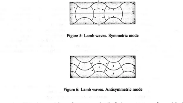
of thickness2h comparable to the wave length, due to the existing coupling between the longitudinal L and transverse TV wave components. In this way, two types of Lamb waves can be produced. The symmetric waves (Figure 5), in which on either side of the middle plane of the plate, the longitudinal components are equal and the transverse components are opposite and the antisymmetric waves (Figure 6) in which on either side of the middle plane of the plate the transverse components are equal and the longitudinal ones opposite. The Rayleigh waves R2 , to be used in the next section, are related to the Lamb waves. They are produced when the plate thickness2h is much greater than the wave length and they are propagated along the free boundary and independently of the plate thickness.
Figure 5: Lamb waves. Symmetric mode
Figure 6: Lamb waves. Antisymmetric mode
According to the general theory of wave propagation, the displacement vectoruof a material point can
be derived from a potential scalarcl>and a vector potential1/J, so that the following relation holds
u=VcI>+Vx1/J
In the expression (2) the two potentials shouldbefulfill the two wave equations
(2)
18 2c1>
VL
~ (c~'r
V2
c1>-
- - = 0 with (3)v2 8t2L
18 21/J
(e.'r
V21/J- - - = 0 with VT= - (4)
v} 8t2 P
withv LandVT are the phase velocities of the longitudinal and transverse waves. The elastic constants
co{3,
a,
(3=
1,2, ...,6 are defined as function of the Young modulus E and the Poisson ratiov
as follows:(1 - v)E
Cll = C22 = C33 = (1
+
v)(1 _ 2v)vE
Cl2
=
C23=
Cl3=
(1+
v)(1 _ v)E Cll - Cl2
C44 = C55 = <=66 = =
-2(1
+
v) 2(5)
(6)
(7)
in which the remaining nonsymmetric terms co{3 (a
#
(3are null.As it is known the stresses and strains associated to the volume changes can be expressed in terms of the function cl> and the stresses producing only shear deformations, without volume changes, can be expressed in terms of 1/J.
It is assumed Lamb waves travel along the axisXl and diffraction in theX3 is ignored. In the case of an isotropic and homogenous elastic solid the scalar and vector potentials are trigonometric functions of time t with the same frequencyw. Then, they can be expressed in the following way, withk the wave number:
cl>= cl>O(x2)ei(wt-k:l:d and 1/J= ['!PO; (x2)]ei(wt-k:l:d ,j = 1,2,3 (8)
A boundary value problem of the waves can be defined by the wave equations for each potential function and the boundary conditions0"2i = 0,i = 1,2,3on the free faces X2 = ±h. In order this boundary value problem can have a non trivial solution, it is necessary that the frequencywand the wave number
ksatisfy the following dispersion relation, called Rayleigh-Lamb equation:
w4 2 [ ptan(ph
+
a)]
- = 4kq 1-~---:-_-...;,.
v} qtan(qh
+
a)where the constantspandqare defined as follows:
1r
with
a
= 0 anda
=-2 (9)
(10)
and the angle constanta can take the values 0 and ~ depending on the type of symmetry of the Lamb wave, as it will be discussed later.
If the relation (9) is satisfied, then the potencial functions can be found, except by a constant factor and their expressions are:
'!Pl = '!P2 = 0, '!P3 = Asin(qx2
+
a)exp[i(wt - kx l )] and cl>= BCOS(pX2+
a)exp[i(wt - kxd] (11)in which the constantsAandBhave to satisfied the following linear homogenous system of simultaneous equations:
dis-placements, except by a constant factorA,at timetof any material point(Xl,X2)of the plate, according to the expressions
[
2k2 cos(qh
+
0') ]UI = qA COS(qX2
+
0') - k 2 2 (h ) COS(PX2+
0') exp[i(wt - kxdl- q cos P
+
0'[
2pq cos(qh+O') ]
U2 = ikA sin(qx 2
+
0')+
k 2 2 (h )sin(px2+
0') exp[i(wt - kxdl -q cosp +0'( 13)
(14)
The equation (9) can be represented in the plane(w,k)and then it defines a curve known asdispersion
curve. In this curve three regions can be distinguished, according to the value of the phase velocity
w
V =
k
is greater either than the longitudinal wave velocityvL or than the transverse velocity velocity VT. Then, the relations (10) can be written as follows:(15)
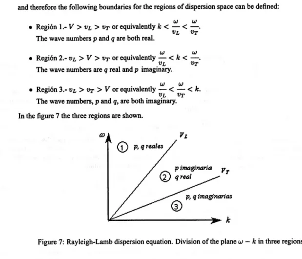
and therefore the following boundaries for the regions of dispersion space can be defined:
w w
• Region 1.-V> VL
>
VT or equivalentlyk< - < -.
VL VT
The wave numberspandqare both real.
w w
• Region 2.-VL
>
V>
VTor equivalently -<
k< -.
VL VT
The wave numbers areqreal andp imaginary.
w
w
• Region 3.-VL
>
VT>
V or equivalently -< -
<
k.VL VT
The wave numbers,pandq,are both imaginary. In the figure 7 the three regions are shown.
l'r
p, q imagi1'!arias
k
Figure 7: Rayleigh-Lamb dispersion equation. Division of the planew - k in three regions
For each of the three above region the corresponding expressions for the displacements when the real components of the expressions (13) and (14) are considered:
• Region 1(pandqare real)
[
2k2 cos(qh
+
0') ]UI = qA COS(qX2
+
0') - k 2 2 (h ) COS(pX2+
0') cos(wt - kxd-q cosp +0'
[
2pq cos(qh
+
0') ]• Region 2 (p is imaginary, i.e.piandqreal) Case a = Q
[
2k2 cosqh ]
UI = qA cos qX2 - k 2 2 h h cosh PX2 cos(wt - kxt} -q cos p
[
2pq cosqh ]
U2 = -kA sinqx 2 - k 2 2 h h sinhpx 2 sin(wt - kXI)
-q cos p Case a = ~
[
2k2 sinqh ]
UI = qA -sinqx 2
+
k2
2' h hsinhpX2 cos(wt - kxt}- q SIn P
[
2pq sinqh ]
U2 = -kA COSqx2
+
k 2 2' h hcoshpX2 sin(wt - kxt}- q SIn P
• Region 3 (p andqare imaginary, Le.piandqi)
Casea=Q
[
2k2 coshqh ]
UI = qA COShqx2 - k 2 2 h h COShpX2 cos(wt - kxt}
+q
cos p[
2pq coshqh ]
U2 = -kA sinhqx 2 - k 2 2 h h sinhpx 2 cos(wt - kxt}
+q
cos p Case a = ~[
2k2 sinhqh ]
UI = qA sinhqx 2 - k 2 2' h h sinhpx 2 sin(wt - kxt}
+q
SIn P[
2pq sinhqh ]
U2 = -kA COShqx2 - k 2 2' h h COShpX2 sin(wt - kxt}
+q
SIn PA particular case of special interest of wave Lamb corresponds to the valuesq2 = k 2. Then the equations (10) lead to the results
w
2W
- = 2k2 -+ V = - = vTV2 (16)
v}
ki.e., as the following relationsVL
>
V>
VT are satisfied, the dispersion curve is in the region2, and then p is imaginary (p = Xi). Moreover the plate velocityVp fulfills the condition(17)
where the plate velocityVp is the limit of phase velocity when the frequency wand k,both approach to zero in a Lamb wave symmetric mode. The equation (17) is valid for every mode except for the antisymmetric mode, represented by Ao, with a velocityV smaller thanVT.
In general, when q = k it can be written kh = n21r with n odd for symmetric modes and even for
antisymmetric modes. The Lame modes appear for equally spaced values of the frequency-thickness product, given by the formula
VT
2hf
=
nJ2'
n=
1,2, ...{·41
"+,
[/S21
Figure 8: Lamb wave (Lame mode) forq2
=
k2.(a) Propagation to 45° (b) Displacements4.2 Numerical simulation. Application
A illustrative example of the application of the Lamb waves as a tool to identify partially penetrating cracks in metallic plates an laboratory test will be numerically simulated.
I't''iII Z0C4
1'l':5e:59
PLOfN:>. 1
~nJ.n'IOi
:ne-.20CE~
tlX IAIA;;)
"""'""
O'X-.IOl£~
9f;-.965Crl)5
9'X-.100E~
""" 12 200408:5G:09 PLOI'to. 1
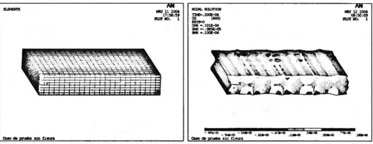
Figure 9: Uncracked plate. (a) FE mesh. (b)Displacements UI att = 2.5 X 10⁻⁵sec
In the following a rectangular steel plate of the following dimensions is considered. Total thickness 2h= 0.02 m, plan dimensionsa= 0.200 m and b= 0.120 m. A train of symmetric Lamb waves(0:= 0 of frequency
f
= 200 X 103 Hz is introduced in the plate trough the side of length a. The material of the plate has the following characteristics: Young modulus E = 1.962 X 10⁸ MPa, Poisson ratio v = 0.3093 and density p = 7.797 t/m3• From these data the angular frequency isw = 1256637.061rad/sec, the transverse and longitudinal velocities are: VT
=
3099.9248 m/sec and VL=
5889.5724 m/sec and from the dispersion equation the wave number isk= 218.1658 m-I and the wave velocity is V = 5760.01 m/sec are obtained. In this particular case the Lamb wave is situated in the region 2, i.e. p is an imaginary number andpis a real one.Using the properties of symmetry of the analysis half plate has been modelled. The FE mesh has been uniform with 24 divisions along the longitudinal direction Xl. 8 divisions along direction X2 and 20
through the thickness (direction X3). The the maximum side length of an element is 0.005 m and the time increment used was 120 per cycle i.e. tlt
=
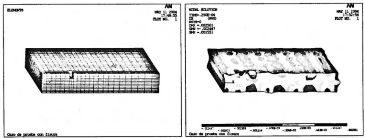
4, 17X 10-8sec. The FE mesh used in the analysis is shown in figure 9a.The displacement results of the wave propagation analysis for a particular time are shown in figure 9b. Similar procedure has been carried out on a damaged plate with a crack parallel to sideaand situated at sectionXl = 0.007 m. The total length of the crack was 0.010 m and its depth was 0.010. The constant
crack width was 0.002 m. The mesh and the results are shown in figures lOa and lOb.Itcan be observed that the dimensions and position of the crack are directly revealed in this analysis2•
"'Y1: lOC4 11:48:55 PlO!'lC. 1
laW..!nJJM0l
~.Z5<Z~
OX (A\C) . . " , . .
CY.IC-.002!l01 9i\-.0C2"41
9«-.001551
Figure10: Cracked plate. (a) FE mesh. (b) DisplacementsUl at
t
=
2.5 X 10⁻⁵sec5 Metallic plates. Superficial cracks
5.1 Elastic plates excited by Rayleigh waves
Rayleigh waves can be used to damage detection of superficial cracks appearing in a plate. Typically, the detection of these superficial cracks or fissures is important due to their relation to structural maintenance and protection rather than to safety requirements. Details of this approach for damage identification can be seen in [SM02l, and therefore only main results will given below.
The Rayleigh waves represent a particular case of elastic waves propagating along a free surface of an infinite half space elastic solid without penetrate into it.
The coordinate cartesian axis areOXi, i = 1,2,3and the infinite half space elastic solid is defined by the domain X3
<
O. The waves are propagated along the boundary planeX3 = 0in the directionOXl. The problem to be solved is a 2-D elasticity, namely in plane strain and therefore only the planeX2=
0is considered, i.e. the one containing the coordinate axisOXlX3'
The waves equation for each componentUof the displacement vector, either longitudinal,Ut,or
transver-sal,Ut,is the following one3:
(18)
wherec
=
vL orc=
VTis the respective wave propagation velocity according to the componentU is a component of the displacement vectorUt or of the vectorUt.The solution of (18) is assumed to be in the form:
(19)
that if it is introduced into equation (18) this one becomes:
(20)
w2
Ifk2 - -
<
0 then the periodic wave is not damped inside the elastic solid and the waves are not c2w
2belonging to the superficial type. Then it is assumed that the condition holds: k2 - -
>
0 and the c2following result is obtained after integration of (20):
(21 )
It should be noticed that for X3 -+ -00 it must f(X3) -+ 0and introducing the parameter4 /-L
~
V
k2 --;;2
the expression (21) becomes into the following one:(22) and then each component of the longitudinal and transversal wave displacement given by (19) becomes: (23) The real displacement vector is the sum of the vectorsUIandUtand their components satisfy the equation
(18) withc
=
vL orc=
VT according to the respective case. The linear combination of both waves is found using the condition that the resultant stresses are zero along the free boundaryX3=
0, i.e. along the boundary limiting the elastic solid. Mathematically this condition can be expressed by the following equation:(1ijnj = 0
in which the index summation convention is assumed and n = (ni) is the unit vector normal to the boundary, in this case this vector isn
=
(0,0,1).Due to the fact that the problem under consideration is a 2-D initial-boundary value problem of the total displacement vectorU = U(Xl' X3) and free boundary conditions at the faceX3 = 0of the plate, i.e. the values for three components of the stress tensor at :
Using a similar procedure as in previous section, but now with the displacements the basic unknowns, that have to satisfy the equilibrium, constitutive and compatibility equations, the following final results related to the Rayleigh waves are obtained:
The relation between the frequency wand the wave numberk or dispersion equation is obtained as the condition of existence of a non trivial solution of the initial-boundary value problem. Its expression is
(24) The condition (24) can be substituted by the following equivalent more convenient equation:
(25) with the notation~andAfor the ratios
x..
and !X.respectively, i.eVT VL
w
~=-vTk'
VT A=-=
VL
1- 2v 2(1
+
v)andpandqare now denoting the imaginary parts of the rootspandq.The unknown~can be found as a root of the equation (24).
As the frequency of the superficial, transversal and longitudinal, waves is proportional to the wave num-ber with a proportionality constant equal to the wave propagation velocityV,then the following equality is obtained: V = VT~.
Using the following equations the constantsp and q are found:
R
2p= k2_2=k~,
vT (26)
Finally the componentes of the transversalUTand longitudinalULdisplacement vectors can be obtained
by using the following expressions:
= =
Ut3
-k(2 -
e)
~ekliXl-iVt+v'1-~2x31= ik(2 - e)ek(iXl-iVt+v'1-~2x31
=
2k~ek(iXl-iVt+v'1->'2~2x31-2ik~
VI -
.x2~2ekliXl-iVt+v'1->'2~2x31(27) (28) (29) (30) A last observation about the dispersion equation.Itshould aware that among the solutions of the equation (25) only the ones satisfying the inequality 0 $ ~ $ 1should be considered, because by definition~is positive and the constantspandqare real. Besides, it is convenient to observe that.xfulfill the condition
o
$ .x $ ~ and therefore only one solution of the equation (25) exists with these characteristics that is within the interval 0,874 $ ~ $ 0,955. Also it is noticed that for depths greater than twice the wave2
length; i.e. for depths X3
< -
k
the displacements are negligible, or equivalently, most of the waveenergy is concentrated along the surface of the elastic solid.
5.2 Numerical simulation. Application
In the numerical simulation of elastic waves several techniques are currently used: Finite differences (FD), Finite elements (FE) and Boundary elements (BE). Each of them has pros and cons. In this work a scheme in finite differences in the temporal discretization and the finite element method for spatial discretization of the continuous model was applied.
.'0" .'0"
-
. -
-< "t.
."
,
."
·c~••
~
-..
...
0.01 G,O'S ••D>..
.,.
....
0.01$..""
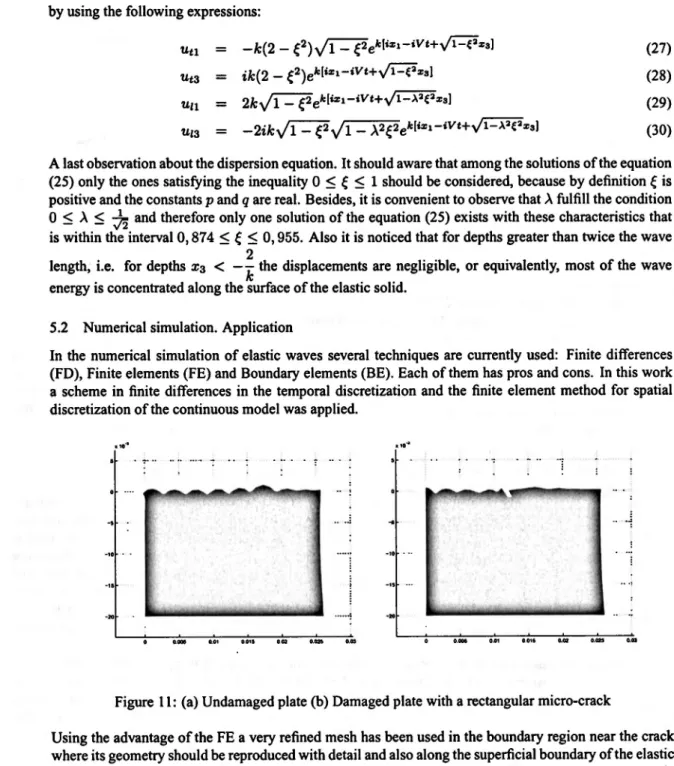
.D>Figure 11: (a) Undamaged plate (b) Damaged plate with a rectangular micro-crack
Using the advantage of the FE a very refined mesh has been used in the boundary region near the crack where its geometry should be reproduced with detail and also along the superficial boundary of the elastic solid, zones with high gradient of stresses produced by the travelling Rayleigh waves. Isoparametric bilinear finite elements have been used with interpolation at the vertices of the quadrilateral elements. A 4 x 4 Gauss integration formula has been considered in the FE matrices numerical evaluation. The spatial discretization leads to a system of a large number of simultaneous ordinary differential equations. In order to increase the accuracy of the solution and eliminate the dissipative and dispersive effects inherent to some FD schemes an implicit unconditionally stable scheme of second order has been chosen. The selected FD scheme is the trapezoidal rule, that belongs to the Newmark family of FD methods with the
1 1
parameters
13
=4
and'Y=2'
This numerical technique has been applied to the simulation of a laboratory test carried out on a alu-minium plate of dimensions in plan 130 x400 mm and thickness 20 mm. The plate material characteris-tics are the following ones: E = 7,41 X 10¹⁰N/m2,p= 2,7X 10³kg/m3andv = 0,3302.The wave
211"
Using these data the following intennediate results have been obtained:
VL = 6379,07 m/seg, VT = 3211,84 m/seg
>.
= VT- = 0,503496, {=0,932053VL
U = 2923,61 m/seg, w= 6269791,88 rad/seg,
f
= 997869HzThe results corresponding to the study of a undamaged plate and the same plate but damaged with a rectangular micro-crack of dimensions: width 6,933 x10-4m and depth 1,25X 10⁻³m are presented. Due to the test characteristics and in order to diminish the computational effort only one fifth of the total plate length but keeping the plate depth, Le. the model dimensions were: £1 = 0.026 and£3 = 0.020 metros.
The FE mesh used in this analysis was composed by 1891 nodes and 1900 elements. The proportion between the numbers of elements in vertical and horizontal direction has been selected nearly equal to the ratio between the height and the length of the model. The mesh has been also refined at the neighborhood of the boundary Xl = O. The time step size was tlt = 2 x 10⁻⁸ and the maximum
simulated time span time wasT
=
3X 10⁻⁶•The computer time was 2460 CPU seconds in a Pentium III of 500 MHz computer.
In figures lla and lIb the behavior of the Rayleigh waves in the damaged and undamaged plates is presented. It can be observed the even very small cracks are immediately detected because the Rayleigh waves stop their travel when they found the obstacle represented by the micro crack. Itis expected that for a 3-D model this property can be used to identify no only the existence of the damage but also its geometry and localization in plan. This type of tests will pennit to maintain the quality of protective painting of plates.
6 Reinforced concrete beams
The discussion in the following parts of this section 6 is concentrated to detection methods of damage in reinforced concrete structures, i.e. to crack identification of structures composed by beams, although some comments can be extended and applied to other more complex structures. Evidently, this issue is a different topic respect to metallic structures damage detection previously described. This difference is due to the non homogeneity of the reinforced concrete and the fact that typically the identification procedure is carried on the already built structures. These circumstances prevent the application of the previously described damage detection methods (use of guided waves and partial dynamic structural ex-citation etc.) to the civil and building structures. Very often these structures are excited to low frequencies vibrations.
As it is well known health monitoring of reinforced concrete beams by using dynamic tests has been a topic of intensive research for the last decades. Typically they are based on the estimation of the changes of a selected dynamic characteristic of the cracked structure, i.e. of a Dynamic System Characteristic (DSC), either natural frequencies, or mode shapes or measured of the dynamic flexibility, in comparison to the uncracked one. A short summary of the use of these DSCs in the damage detection methodology is given. The inherent models for the cracked beam behavior are also discussed. Currently, the effect of crackinginthe free vibrations of a concrete beam is analyzed according to one of the following three approaches. Inthe first approach it is assumed that the cracks width and pattern remain unchanged during the beam vibration. In the second approach a bilinear behavior for the beam is considered, namely, the beam behaves as uncracked or as cracked depending on the crack is closing or is opening respectively. Finally, the third approach uses a time dependent model in order to replicate the variation of the closure and opening of the cracks by the introduction of a set of discrete springs. Most of the detection damage models for reinforced concrete beams uses the first approach, that implies the fulfillment of the following assumption: the beam vibrates with small amplitudes around cracked static equilibrium states. This hypothesis can be accomplished in many dynamic tests of structures in the field. However, despiste of this fact recent contributions considering the nonlinear concrete behavior has been published [RabOl] and [MFH+90].
This section is finished by a comparative study among the different DSCs commonly used. Itcan be observed that, in general, differences between uncracked and cracked beams are small and some they can not be distinguished from the inherent measurement errors occurring during the tests.
multiple and non symmetric cracks in order to cope more realistic situations. Finally, some comments about the identification methodology are also given.
6.1 Dynamic system characteristics
In general, the crack presence in a structure reduces its natural frequencies and increases its damping respect to the uncracked structure. By comparing the results of these DSCs obtained in the pristine structure (or in a theoretic model, usually in FE) and the ones found in a dynamic test in the cracked structure is ideally possible by comparison to detect the presence of structural damage, crack position and severity. This identification process implies to solve an inverse problem, that demands previously the construction of a structural model for the dynamic behavior of the damaged structure. A very simple model of this type is to reduce the elasticity modulus do the damaged elements of the structure, although there exist more realist alternative models, in which the crack presence is better simulated.
In important point in a damage detection method is the selection of DSC to be compared. In the following the merits and drawbacks of some possible choices are discussed. In this respect different DSCs have been used. For example, in addition of the reduction of the natural frequency and the modification of modal shapes0 their derivatives, the response function in the frequency domain, wavelet transforms and
the power spectral density, among others have been analyzed. Also in same occasions a multiple criteria for damage detection has been applied, in which several DSCs has been considered. Obviously, the selection of the DSC depends in each case on the identification procedure used, as error minimization, penalty function, use of genetic algorithms [ASM04], neuronal networks approximation [KH03] etc.
6.2 Natural frequencies
Measurement of natural frequencies is an inexpensive and quick procedure for structural damage detec-tion. One advantage of this DSC is its global character, because any localized crack in the structure can be in principle revealed by this measurement. However, the sensitivity of the frequency to the damage may depend on the its severity and its localization. For example, if the crack is concentrated near a node of the vibration mode of the natural frequency, then the stress modification produced by the crack presence is very small. Then the damage sensitivity for the natural frequency considered is very low. Contrary conclusion results, if the damaged area coincides with the modal crest. Summarizing, damage represents a stiffness reduction and therefore a decrease of the natural frequency. Moreover, if damage increases, either in number of cracks or in their severity, also the natural frequency diminishes.
Normally, small cracks can not be detected easily, because the difference between natural frequencies of the undamaged and damaged structures is very small and it may be originated by other causes (temper-ature, traffic noise, measurement accuracy etc.). Therefore, it is usual to admit cracks existence if the difference is greater than 5 %. However, it is possible to measure natural frequencies at different phases along the life of the structure, and in this way, to evaluate the damage degree, or at least its progression, if damage already exists and differences are increasing with time. Sometimes, the measured frequencies are greater than the theoretical ones. In these cases there exist an increase of the structure stiffness, usually in its supports.
An aspect to be considered when frequencies are used as DSC is referred to the choice of its most suitable order. There is a lack of consensus on this point. Low order frequencies are simple and easy to obtain in a test. However high order frequencies generate complex modes of vibration, suitable to detect damage. Related to this issue is the selection of the frequencies number to use in the test and in the damage identification algorithm.
An important limitation of the use of this DSC is to assume a particular structural damage, a crack, that is modelled by a hinge. This model prevents the identification of other types of damage, as steel corrosion, that does not modify significatively the natural frequency of the structure. Similar comment can be applied to structural damage caused by stress losses in prestress tendons, unless in the dynamic tests on the undamaged and damage structures an additional accompanying load is introduced in order to reveal this type of damage. Finally in symmetric structures the computed damage position may be not be unique.
The relation between the changes of the stiffness of the structure and the natural frequencies can be found by using the shape vibration modes of the uncracked structures as follows:
Let it be Wi and (jJi the natural frequency and the corresponding mode of vibration of orderi. Itis assumed that the mode is normalized respect to the mass matrixm of the uncracked structure, i.e. the following condition is satisfied:
<pr m(jJi = 1
In addition, each modei is solution of the equation
and by pre-multiplying by(jJithis equation becomes:
(jJrk(jJi = Ai(jJr m(jJi = Ai
(31)
(32)
(33) The stiffness matrixk of the pristine structure is modified to the matrix kdof the damage structure, that
can be written, kd = k
+
6kand it is assumed that damage does not modify the mass matrix of thestructure.
The new modes of vibration of the damage structure should satisfy the normalizing condition (31), that is simplified in the following expression, if second order terms are neglected.
The above equation can be written in the following way:
(k
+
6k)((jJi+
6(jJi) = (Ai+
6Ai)m((jJi+
6(jJi) -+k6(jJi+
6k(jJi = Aim6(jJi+
6Aim(jJi (35)and pre-multiplying by(jJr and using the relation((jJi
+
6(jJi)T(k+
6k)((jJi+
6(jJi) = Ai+
6Aithe final expression that relates the frequency change6Aiin terms of the changes of the stiffness matrix(36) Itis a common hypothesis to express the stiffness matrix of the damage structure in terms of the distinct element matrices affected by a factor,{3j, called damage coefficient, that reduces the elasticity modulus of the damaged elementj,i.e
m
kd = L{3jkj
j=l
with m the number of elements that can be potentially damaged and 0$ {3j $ 1.
(37)
6.3 Frequencies and static test data
The damage detection based on static tests are simpler than the ones based on dynamic tests, because the static equilibrium equations stiffness is the relevant property. Moreover, the costs of the dynamic test are higher than the ones of a static test.
Some damage detection methods uses hybrid tests as in [WHFYOI]. Inthis work the damage identifica-tion is carried out in two phases. In the first the changes of natural frequencies are used and afterwards the displacements of the structure are measured under different static loading cases. With these two groups of data and the tentative assumption of equal severity of damage it is possible to identify the damaged zone of the structure,. Then, once the damaged zone has been tentatively identified the intensity of the damage can be estimated.
The main idea of this combined damage identification method consists to test the structure under sev-eral loads combination. The damage identification uses the comparison between the measured static displacements and the frequencies in the undamaged and in the damaged structure. For both groups of results the changes due to the damage is computed using a first order approximations as follows:
• Static displacements u in the undamaged structure
• Static displacementsud in the damaged structure
(39)
then
t5u= u - ud = k-1t5kk-1p
and the damaged matrices are affected by the corresponding damage factors
p.
Similarly, the natural frequency can be evaluated according (36).Several identification algorithms,[HS97] and [SS91], for damaged elements, that use the minimization of an objective function of quadratic error type have been used in applications. However, two main sources of errors exist in the static tests. (I) The information from a static test is more scarce than a dynamic test, and therefore it makes more difficult to obtain reliable results in the identification procedure. (2) The damage effects can be cancelled due to the limited number of load paths. For example, an existing damage can not be revealed for a particular load case, if its effect is small in the global deformation of the structure. In order to avoid these difficulties several alternative procedures have been developed, that can generate automatically the load cases to be tested, in such a way that potential damages can be detected.
6.4 Frequencies and mode shape derivatives
An important point in damage identification is to establish a correct correlation between the DSCs mea-sures from the test and the damage existence, localization and severity. In general any local or global damage is associated to structural changes, that can be observed through changes in the DSCs.
In addition to natural frequencies as DSCs another damage indication can be the direct comparison between modes, or their first derivatives or in some cases their curvatures. The main difficulty in this approach lies on a suitable selection of the order of the modes used to reveal the damages or, in the case of first derivatives and curvatures of modes, on the ability to obtain a sufficiently accurate measure of these DSCs. In [DT04] a numerical simulation using curvatures and natural frequencies computed by EF with error estimation and re-meshing techniques to improve the solution have been presented Then, several methods have been proposed to establish the former correlation. Some of them, with reference to reinforced concrete beams, are commented below.
• Modal Assurance Criterion(MAC) and Coordinate Modal Assurance Criterion(CaM AC). These derived values from the DCSc are defined by the expressions
m
I
L)cP~i)(cP~i)12
j=l
COM ACi
=
"""':m=-'---=m::----~)~y~)cP~y
j=l j=l
(40)
in which Cl>A = [~l with j = 1,2, ... ,mA the matrix ofn x mA dimension, containing the
mA modes od vibration that have considered in the test A and similarly the matrix Cl>B = [<p~l of dimensionn x mB of the testB is defined. The components of the mode,<p~,column vector of dimension
n,
are written as<p~ = (cP~i)withi = 1,2, ... ,n
and similarly for the testB. In the expression ofCOM ACit was assumed the existence of m vibration modes common for both tests.The value ofMAC varies between 0 and 1. IfMAC = 1then there exists a total correlation between both tests and when this value approaches to zero means there is structural damage. The valueCOM ACis often used to identify the structural mode from two sets of measurements do not correlate. Values close to I show a correlation for the modal coordinatei and small values are indication od damage existence.
• Method of strain energy.
energy ofN finite elements, that divide its length, according to the expression:
( )
2
aj+l
{}2</J-with U- -=
1
El- - - ' dx'} a-
,
}ax
2 (41)For each element it can be defined its proportion of strain energy respect to the total strain energy of the beam by the following formula:
(42)
in which the average stiffness of the elementj and the average stiffness of the beam are denoted byElj andElrespectively.
The variables related to the damaged beam are identified by the superscriptdand the following relations can be written:
(43)
In order to use them vibration modes considered in the test it is defined the damage index for the elementkas follows:
m
'LT:k
{3k = i=lm (44)
'L7ik i=l
The damage index gives an indication about the health of a structure, because{3k represents the deterioration degree of the bending stiffness of elementkdue to the change of the stored energy in the structure caused by a particular vibration mode. Itis assumed that the indexes{3k represent a random variable with normal distribution. Then it is possible to define a normalized damage index as:
{3k - {3k
Zk = - - - (45)
with{3k and Gk are the mean and standard deviation of the damage index population. • Method of the flexibility
The presence of a damage in a structure increases its flexibility. Then, based on this fact it is possible to compute the flexibility matrix of a structure from the knowledge of its n vibration modes measured in the tests. These modes are assumed to be normalized respect to the mass matrix, rn, i. e. they fulfiU the condition fori = 1,2, ...
,n:
The stiffness matrix k and the flexibility matrixf of the system are:
(46)
where
<p
is the matrix containing thenmodesas column vectors andn
= diag(w;.Therefore, if f and fd are the flexibility matrices of the pristine and damaged structures respec-tively, then the following matrix damage indicatorDoFcan be defined as the difference
(47)
damage identification and its location is carried out according to the maximum values of each column of the matrix.
• Method of the residual dynamic forces
Finally, there exist other procedures that use the modal measurements of the test in a different way than standard methods in order to obtain, for example, the residual dynamic forces. Then it is possible to define a new objective function tobeminimaze in the damage identification process. This interesting concept expresses the dynamic equilibrium that should satisfy a structure subjected to free vibrations. This procedure will be summarized in the following.
The displacements of an undamped structure with n degrees of freedom is governing by the system of differential equations
mii+ku = 0
and for the natural frequency of orderi the following equation is satisfied
k<Pi -
w?m<Pi
= 0(48)
(49)
When damage occurs the matrix of the uncracked structure k becomes intokd. As it has been
already discussed, expression (37) this matrix can be expressed as sum of the element matrices, each multiplied by a damage coefficient
f3;,
i.e.m
kd =
Lf3;k;
;=1
(50)
with m the number of potentially damaged elements and 0
:5
f3;
:5
1Assuming the mass matrix remains constant if damage occurs and the corresponding frequencies and modes of the damaged structure satisfied the following equations, for each frequency:
(51)
From the former equations the residual dynamic force vector for the mode i, can be expressed approximately:
m
Ri = -(wf)2
m<pt
+
L f3;k;<Pt
;=1
(52)
The vector of equation (52) will be zero if the correct values of the damage coefficients
f3;
at each element j are introduced and the exact information about the values of the frequencywt and the mode vector<Pt
of orderi as well. This equation is valid for all frequencies and modes (i= 1,2, ... ,n)and al of then can be written explicitly in the following way:Rh
kf1 - (wt)2 mll kf2 - (wt)2 m12 kfn - (wt)2 m1n<Ph
R
2i kg1 - (wt)2 m21 kg2 - (wt)2 m22 kgn - (wt)2 m2n <P2i= (53)
Rni k~l - (wt)2 mn1 k~2- (wt)2 mn2 k~n - (wt)2 mnn <Pni
Itcan be shown that the terms ~iare zero if the matriceskdand m are real and symmetric, and
then from the former results is possible to build the following objective function to be minimized:
(54)
6.5 Comparative study
The first occurs due to the fact that significative damage can cause small changes on the frequency values and these changes can be overlooked and mixed up with other causes like the instrument precision The other limitation is caused by the uncertainty related to changes of environment or in the structure mass distribution.
An alternative DSC to the frequency is to use the information on changes in the vibration modes when a damage occurs in the structure. The advantage of this procedure lies on the higher capability of the modes to capture local damages than the frequencies. However, this DSC presents some inconveniences. The first, the damage, typically a local phenomenon, may not affect significatively to a mode of a particular order. This can happen in modes of low order, that are common in the free vibration of civil structures, usually of large mass and stiffness. Another inconvenience corresponds that the mode shapes, may be, can be also affected by the environment conditions, traffic loading or inconsistent positions of the measurement sensors. Finally, the number od sensors and their positions can also have importance on the accuracy of the procedure of damage detection.
In relation to the remaining DSCs in the publication (NVH02] a study based on some of the former derivatives of modes of reinforced concrete beams have been carried out. From this study the following conclusions have been drawn.
• The natural frequencies of a reinforced concrete beam are sensitive to damage accumulation, Le., to the presence of new cracks, but not to the their position. The frequency decrease is monotonic and this property is a good indicator for estimation of damage intensity evolution along time. • The indexes are less sensitive to damage than the natural frequency but they can give a good
indication about the symmetry or antisymmetry of the damage.
• From the evolution of the indexesCOM ACit is possible to detect and localize the damage in reinforced concrete beams, but the decrease of these indexes can not permit the evaluation of the damage intensity and its extension.
• When the damage is not local and therefore concentrated at a section, Le. it is extended to several elements, the decrease of the flexibility as indicator can not permit an easy localization of the crack, but can be valid for its detection
• With the use of the damage indexes it is possible to detect and localize in reinforced concrete beams local damages, non extended cracks, in a mor precise way than with the application of other methods likeCOM ACand f1exiblity. However, it is very difficult, like in other methods, to localize cracks when they are extended. In any case, the crack severity evolution can be tracked by means of the computation of the natural frequencies.
7 Elastic model of the beam with cracks 7.1 Introduction
The theorem of Hu-Washizu (H-W), developed independently in [Hu,55] and [Was82], has been applied in [CB84] in order to derive the Navier Bemoul1i (N-B) beam with cracks subjected to free vibrations. The obtained approximated damaged beam equations are dependent on an estimated function cal1ed crack function. In this way the presence of a crack in the beam is simulated by a continuous reduction of the stiffness of beam cross-sections, significative important near the crack. This stiffness reduction is dependent on the crack position and its depth. Then, it is possible to model the cracked beam using the FE method and with this model to identify both, crack position and severity, by solving the inverse initial boundary value problem of free vibrations as is reported in [SFE02]. Here, in this paper the former formulation has been extended to cope the situations of several cracks and non symmetric damage, i.e. cracks situated only in one of two free faces, bottom and top faces, of the beam.
The variational equation represented by the theorem of(H-W) is specialized to a straight uncracked beam ofNavier-Bemoul1i. The fol1owing notation for the beam is introduced
I. A cartesian rectangular coordinate systemOxyzis considered.
2. The abscissae axisOxcoincides with the straight beam axis. The axesOyandOzare paral1el to the principal axes of the beam cross section of the beam.
3. The origin0 of coordinate axes is the gravity center of the left end cross section of the beam. 4. The displacement field of the beam isu, v, w.
5. The distributed forces fz
t-
0, paral1el to axisOz,are acting per unit of volume. and the hypothesis ofNavier-Bemoul1i are summarized as fol1ows:I. The displacement field is defined by the relations
u = u(x, z,
t),
v= 0, w= w(x,t),
u= -zw' (55)in whichh'denoted the first derivative of a generic functionhrespect to abscissaxand
h
its time derivative.2. Then the strain field is
en = -ZK with K = K(X,t)
withK the curvature at sectionx.The remaining strains are
3. The stress field is written as
C7xx=
-zm,
C7xz = C7xz(X,z,
t) with m =m(x,
t)(56)
(57)
(58) in which m represents the bending moment at sectionx divided by the second moment of the section.
4. Final1y the velocities field is defined by the equations
Px = 0, Py= 0, pz = p(x,t) (59)
where the function p(x,t) express the fact that only translational inertial or D'Alambert forces along the axiszare considered. Inertia forces caused by rotation of beam sections are neglected. If the former fields of the beam variables are introduced in the variational formulation of the H-W theo-rem the classical equation for the dynamic vibration of a beam is obtained.
(Elw")"
+
ApUi = f(z) (60)7.2 Navier-Bernoulli beam with cracks
The former formulation for the uncracked beam can be extended to the case of a beam with only one crack as it is shown in figure 12.
Z
6
I
Figure 12: Beam with a crack
Itis assumed that the crack presence modifies only the strain and stress fields respect to the fields of the uncracked beam. Moreover, this modification applies only to longitudinal strains and stresses, i.e. toaxx
and toC:xX 'Then the existence of the crack does not modify the velocity and displacement fields. Therefore, the following fields are assumed, with
f
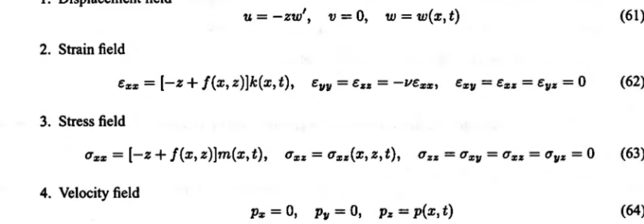
(x, z)a function to be estimated called crack function:I. Displacement field
2. Strain field
u=-zw', v=O, w=w(x,t) (61)
C:xx
=
[-z+
f(x, z)]k(x, t), C:l/l/=
C: zz=
-VC:xx , C:Xl/=
C:xz=
C:l/Z=
°
(62)3. Stress field
axx
=
[-z+
f(x, z))m(x, t), axz=
axz(x, z, t), azz=
aXl/=
axz=
al/Z=
°
(63)4. Velocity field
Px
=
0, Pl/=
0, pz=
p(x, t) (64)The application of the H-W theorem to this case leads to the following equation of the cracked N-B beam of lengthL:
[E(I - Kll)Hw"]"
+
pAw=°
en x E (0,L) (65) that represents the general equation governing the dynamic behavior of N-B beam with one crack sub-jected to free vibrations. The following notation has been used(m,n
=
0,1,2, ...)withb(z)the width of the constant section at coordinatez.As particular cases, the area isA
=
K oo and the second order moment is1= K20 •The function H(x) is expressed in terms of the former functions as followsH(x)= 1- K ll 1- 2Kll
+
K02 The boundary conditions are formulated as follows:• Static or force conditions
-Ml/
+
€(Kll - I)EHw"=
0, Qz - €(I - KllE(Hw")'=
°
with€=
-1 ifx=
°
and€=
1in the casex=
L.• Kinematic or displacement conditions
w' =
-8,
w=w
(66)
Itcan be observed that in the case of uncracked beam the crack function f = f(x, z, t)is null and there-fore Kll = 0 and K02 = O. Then, the differential domain equation (65) and the boundary conditions, (66) and (67), become to the well known N-B equations.
By inspection of the domain equation (65) and the boundary conditions, (66) and (67) it is realized that the behavior of a beam with a single crack at an specified section is similar to the behavior of an uncracked beam of longitudinally variable section. The variation law of the equivalent second order moment,Ieq(x), is given by the following expression:
I -Kll Ieq(x) = (I - Kll)H with H = ~--:-:",....---::-:-
1- 2Kll
+
K02(68)
From the fonner discussion it is obvious the importance of a suitable selection of the crack function in order to model adequately the dynamic response of a beam with crack. In the next section this topic will be discussed
7.3 Crack Function
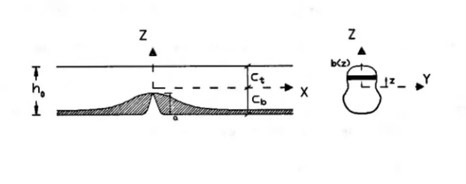
The case of a beam of symmetric constant cross-section with two symmetric cracks, one at each face, bottom and top, of the beam with equal depth has been studied by [CB84]. The crack function obtained by physical reasoning was an exponential function. Here this result will be extended to cope other crack pattern. First, the presence of a single crack appearing at one of the two faces of the beam is modelled. Then, the existence of several cracks, each of different depth, will be considered. In all cases it will be assumed constant cross-section of the beam, although nonsymmetric. In the figure (13) the notation and the system of coordinate axis used in this case are shown.
Z
A
z
Figure 13: Crack function. Beam with constant nonsymmetric cross-section
The data used to define the model when the crack is situated at bottom face are crack positionXi and depthai. The gravity center of the constant cross-section is defined by the distances, Ct andCb,to the two faces, top and bottom, of the beam respectively. Then, the beam height ish
o
such thatho
= Ct+
Cb. The width variation of the section is given by the functionb(z)of the coordinatez. In the following two dimensionless variables are introduced: the ratioJ1.between the second order moments of the uncracked section and the cracked section andthe relative abscissa u. Both are defined by the expressions:(69)
withZgi the gravity center of the cracked section, that can be found by the fonnulae
J~~b+a,
b(z)zdzZg = -J';;;C;7,
'-.:--::.'--b(':'"""z":""")d-z--Cb+a,
and a is a parameter to be estimated by experimentation. The value 0.667 x 2
=
1,334 have been suggested in [CB84].• At cracked sectionx = Xi there exist two limits, a bottom and a top limits, for the effective section, given by the expressions
z~ = et,
• At a far away section from the crack, in theory atX = 00, the effective section is the whole uncracked section, Le.
• Assuming an exponential variation of the limits of the effective section, the limits for a generic section of abscissaxare:
The extreme longitudinal stresses,a xx ,vary along the beam according to the following considerations: • At sectionx = Xithe stresses are
• At a far away section from the crack
• At a generic section defined by the abscissax
( ) ( 0 00) -u
+
00 _ () _ ( 0 00) -u+
00axt = axt x = axt - axt e axt, axb - axb x - axb - axb e axb
The stress at a fiberz of section x can be found by interpolation from the former values:
(70) with
H[z -
Zb(X)] the Heaviside function andTJ an dimensionless function of the coordinatez,
with values in 0,1).They canbedefined according to the expressions:and the value of the crack functionf(x, z)is, according to its definition:
f(x, z) = -z
+
axs(x, z) (71)Once determinate the crack functionf(x,z)thee characteristics of the equivalent section can be obtained by computation of the following integrals over the whole section of the beam (numerical evaluation is advisable):
1
%·(X)Kmn(x) = b(z)zm r(x, z)dz
%b(X)
in whichA= Kooand / = K20 . The functionH(x)is
H(x) = / - Kll / - 2Kll
+
K02 The equivalent second moment/eq of the section x is/eq(x)
= (/ -
Kll)HA possible simplification is to introduce a linear expansion in e-u•Then is is obtained: f(x,z) = 7(z)e-U
(72)