Techniques for Area Discretization and Coverage in Aerial
Photography for Precision Agriculture employing mini
quad-‐rotors
João Valente, David Sanz, Jaime Del Cerro, Claudio Rossi, Mario Garzón, Juan David Hernández, and Antonio Barrientos
Centre for Automation and Robotics (UPM-‐CSIC), Universidad Politécnica de Madrid
C/ José Gutiérrez Abascal, 2 28006 Madrid, Spain (e-‐mail: [email protected]).
Abstract: Remote sensed imagery acquired with mini aerial vehicles, in conjunction with GIS technology enable a meticulous analysis from surveyed agricultural sites. This paper sums up the ongoing work in area discretization and coverage with mini quad-‐rotors applied to Precision Agriculture practices under the project RHEA.
1. Introduction
In recent years, precision agriculture (PA) researchers have found that the use of unmanned aerial vehicles (UAV) based on quad-‐rotors could significantly help in improving research in agricultural sciences. Their motivation was conceived by its availability, simple assemblage and maintenance, as well as their low cost compared with traditional tools (e.g. Satellites or conventional aircrafts).
The main aim of an aerial survey is to obtain aerial images of the field, which can be used for generating generate a map of the surface though mosaicking procedures, those maps can also be post-‐processed to extract interesting information (e.g. biophysical parameters, shape and features detection).
Aerial robots are mainly employed in agriculture for crop observation and map generation through imaging surveys (Herwitz et al.,2004). The maps are usually built by stitching a set of georeferenced images (i.e. orthophotos) through mosaicking procedures. Typically, they rely on the information about the biophysical parameters of the crop field.
Moreover, the agricultural experiments reported with aerial vehicles fall mainly in waypoints based navigation (Nebiker et al.,2008; Zarco-‐Tejada et al.,2008; Valente et al.,2011), where the drones navigate autonomously through a pre-‐defined trajectory, composed by a set of points in the environment.
This paper have been written as follows: After this brief introduction, Section 2 introduces the conceptual aerial framework with all their components and workload. Section 3 presents the techniques of area decomposition, Section 4 explains the area coverage approach, Section 5 presents some case studies and Section 6 provides an improvement for the coverage path planning with multi aerial robots. Finally, Section 7 reviews the issues summed up.
2. Aerial Framework
The conceptual aerial framework is denoted as a set of actions and components (i.e. software and hardware) that provide the achievement of a task inside a particular context in a feasible fashion. Hence, the framework intends to support area coverage missions with aerial robotic systems in PA practices. This is a preliminary phase in the design of a robotic system that can be seen as a top-‐down approach for solving the problem (i.e. through a step-‐wise design). Abstractly speaking: Breaking up of overall goal, individualizing the requirements, coming up with a concept, and finally starting the design phase.
As it was introduced in section 1, there is an agricultural task demand and a fleet of aerial and ground robots to carry out the proposed task is assumed. To make the concept description easier to follow, let’s assume that there is a general weed control task. This task falls mainly in two sub-‐tasks: the perception system (i.e. identify the weed species and patches over a wide agricultural area) and the actuation system (i.e. kill the weeds). The second sub-‐task will not be discussed since it is not considered in the framework design.
In order to identify the weed species and patches, the agricultural field has to be previously surveyed with an image sensor. In this way, the aerial framework will be responsible for performing this operation.
The framework must be able to provide the operator in charge with the required tools to carry out the mission. This is made up of an aerial vehicle with way-‐points navigation features, a visual sensor, a control station with tools to define and monitor the mission, and finally a mission planner to generate the aerial trajectory. The general inputs for the mission are: Number of aerial units available, field map characteristics (e.g. coordinates, undesired areas), and images resolution and overlapping. The step-‐by-‐step mission can be summed up follows:
1. The aerial units and the control station are setup near the target agricultural site 2. The operator introduces the before mentioned inputs to the mission planner 3. The operator launches the mission planner
4. The mission planner computes an aerial trajectory and sends it to the operator 5. If the operator does not agree with the generated path, the procedure will jump back to 2.
6. Otherwise, the plan is sent to the aerial vehicles, the execution starts, and the operator supervises the mission until finished.
Figure 1 -‐ Mission workflow.
3. Workspace definition and sampling
information enough to obtain the geographic coordinates from the bounds of the field and therefore the field dimensions.
The second step is to define an image resolution and overlapping for the image survey. Once those parameters are defined, the image sensor resolution that better suits the goal then chosen.
After those two steps the number of images to be taken by the robots and the corresponding geographic position within the field are obtained.
The workspace decomposition in the very end is defined as an approximate cellular decomposition, following the taxonomy proposed by (Choset, 2001), which means that the workspace is sampled like a regular grid. This grid-‐based representation with optimal dispersion is reached by dividing the space into cubes (i.e. cells and therefore image samples), placing a point in the center of each cube (i.e. centroid of each image, and therefore a geographic coordinate denoted as a way-‐point). The geographic coordinates from each photograph are computed with the accurate geodesics Vincenty's formulae (Vincenty, 1975).
The last parameter required for the aerial mission is the height of the aerial robots height above the ground. This parameter is computed by considering the cell dimension in the world, and the digital sensor characteristics.
Another advantages of having a grid-‐based decomposition is that it directly maps the robot workspace into a kind of unit distance graph, denoted as grid graph G(V,E) where V denotes the vertices and E the edges. Each vertex represents a waypoint and each edge is, the path between two waypoints u and v such that u ~ v.
4. Area coverage approach
The approach proposed split into in two sub-‐problems: 1) the area sub-‐division and the robot assignment problem are handled. 2) the coverage path planning problem is considered. In Figure 2 the proposed approach is shown schematically where the sub-‐problems are also decompose in two stages.
Figure 2 -‐ Overall approach.
4.1. Area sub-‐division and the robot assignment problem
The multi coverage path planning problem is formalized by assuming that there is a top level procedure that handles the area division and robots assignments (Rossi et al., 2009). For a better understanding an example is shown in Figure 3. The agricultural field depicted has an irregular shape, and has been decomposed in three sub-‐areas, assuming that there is a robot per area with different characteristics and/or parameters.
Figure 3 -‐ Example from the area-‐subdivision approach.
employed where l stands for line segment, ε is an error term and δ stands for cell size. Let's consider P as the end-‐point of a line segment l. The leftmost and rightmost end-‐points of l are denoted respectively by Pl and Pr.
Figure 4 – Borders representation algorithm based on the BLA.
4.2. Coverage path planning
In order to obtain a complete coverage path with the minimum number of turns, subject to a pre-‐defined initial and goal position, and without re-‐visited points within the workspace, heuristic and non heuristic algorithms are employed.
Then, a Deep-‐limited search (DLS) to build a tree with all possible coverage paths is applied in order to find a complete coverage path that passes only once through all nodes in the adjacency graph. Using this approach, the search length can be limited to the number of vertices, and consequently, the search neither goes around in infinite cycles nor visits a node twice.
During the gradient tracking, the algorithm finds more than one neighbour to choose from with the same potential weight. Additionally, the bottleneck caused by the local minimal can also block the search. In order to solve these issues, a backtracking procedure was employed.
Finally, the coverage path with the minimum number of turns is chosen through the following cost function,
Where,
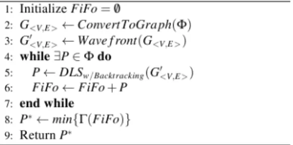
The algorithm pseudo code is shown in figure 5.
Figure 5 -‐ Coverage path planning algorithm. Φ is a field sampled in a finite number of way-‐points, P is a complete coverage path.
Although the gradient-‐based approach does not ensure an optimal solution, it provides a simple and fast way to obtain a near optimal coverage solutions, in both regular and irregular fields, with and without obstacles within, subject to the aforementioned restrictions.
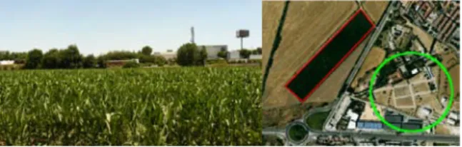
In order to prove the efficiency of the proposed approaches two experimental scenarios with different characteristics were chosen. The fields considered are a maize field (Figure 6) with an area approximately of 20000 m² and a vineyard parcel (Figure 7) with an area of approximately 63765 m², both located in Madrid, Spain.
Figure 6 -‐ Maize field (red square) and UPM-‐CSIC headquarters (green circle).
Figure 7 – Vineyard parcel.
5.1 Aerial Coverage Metrics
The approaches proposed are evaluated through the following metrics: total of area coverage (%), coverage time (s), computational time (s).
For the total of area covered a Quality of Service (QoS) index was defined, and indicates the percentage of the remote sensed field. The QoS index is given by Ub/(N.M)(%), where Ub is the upper bound of the number of unvisited cells, in a NxM dimension grid.
5.2 Maize field (regular shape)
Figure 8 -‐ Result from the negotiation between the robots.
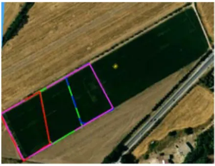
The sub-‐division is then rasterized over the sampled workspace, and for each sub-‐area, a coverage path is computed. The final result is shown in Figure 9.
Figure 9 -‐ Borders representation and CPP computed for each sub-‐area.
In the first sub-‐area, this is from cell 1 to cell 33, a minimum number of 14 turns were achieved. In sub-‐area 2, of cell 38 to cell 65, the total number of turns was 15. Turns. And in sub-‐area 3, cell 76 to cell 100, 14 turns were required. The computational time required for computing each coverage path for each of the sub-‐areas was approximately, 0.82s, 0.34s, and 0.50s, respectively. With regard to the QoS index, there is an upper bound (Ub) of 20% of non covered cells defined as security strips, therefore a QoS of 80% was achieved in this experiment.
5.3 Vineyard parcel (irregular shape)
borders that break down the overall area have to be discretized, but also the contour of the overall area (i.e. which separate the area of interest to cover from the area of non interest).
Considering a step forward of the study, a real mission has been set up with three mini aerial robots, denoted as quad-‐rotors. The goal of this mission was to measure the coverage mission time, considering the short mission range of each drone. The quad-‐rotors considered in this mission were two Hummingbirds, and one Pelican, from the German company, Ascending technologies.
The results from the sub-‐area decomposition are shown in Figure 10 where the characteristics and parameters of three real quad-‐rotors have been considered.
Figure 10 -‐ Sub-‐area decomposition considering three real aerial vehicles (quad-‐ rotors)
The output shown in Figure 10 has been rasterized once again in a grid workspace (10x10 cells). For each sub-‐area, a starting point (e.g. take-‐off) and final goal point (e.g. landing) locations have been predefined before computing each coverage path. All trajectories have been computed in less than 20s. The computed coverage trajectories are shown in Figure 11. A minimum number of turns ranging from 8 to 20 have been obtained. The average coverage time of the three robots is 222s at a velocity of 5 m/s. The average battery consumption during the coverage task was approximately 15% for each robot. The QoS achieved in this experiment is 82% with a Ub 18% uncovered cells from.
Figure 11 -‐ Rasterization and area coverage in an irregular field.
6. Discussion about the amount of area covered
The rasterized borders represented in a multi robot workspace are of great importance, since they work as security strips, where vehicles are not allowed to enter. However, as seen before, a considerable percentage of area when using them remains uncovered. The metric that address the percentage of area covered is the QoS index. Therefore, borders have to be considered so as to improve the QoS but at the same time, safety for the robotic system has to be ensured. A Risk Analysis (RA) has been carried out with the purpose of improving this index.
Defining risky situation as a situation where two or more aerial robots are located in adjacent cells, which makes the distance between them beyond a certain value. Lets denote Pn(Xn; Yn; Zn) the 3-‐dimensional position of a n aerial robot in an aerial fleet with N elements. A risk condition can be written as,
where i is the ith neighbour robot and j the length of a certain neighbourhood. Finally, Δ is the distance between the robot n and a neighbour robot i, and δ a stipulated minimum safety distance that has to be defined.
Secondly, let’s suppose that a robot is adjacent to another (i.e. neighbour cells). For example, the vineyard has an area of approximately 63765 m² which corresponds to 195m length and 327m width. Let’s assume that the aerial robot carries a commercial digital camera that provides image resolutions up to 10.4 mega pixels. Moreover, if choose the best image resolution to sample the field is chosen, it corresponds to an image size from 3368x3088 pixels. If the mission requires a certain percentage of overlapping, the effective size of the image will be reduce in same percentage. If a spatial resolution of 1 pixel/cm is required, a grid resolution of 6x10 cells (each cell will have a dimension of 32.7x32.5m)is obtained.
With these magnitudes a collision between two aerial robots would hardly ever occur. Even considering a position accuracy of 3m and wind speeds of 10m/s, there is no possibility that two aerial robots collide.
In conclusion, whenever a coverage mission where the cells dimension are above a margin of 2 times the robot position accuracy, the security strips can be removed from the planner and a QoS of 100% is achieved. Figure 12 shows the same coverage path computed in Figure 11 but without borders, where the borders have been distributed to each sub-‐area in a load balancing fashion.
Figure 12 -‐ Multi robot coverage without borders.
7. Conclusions
These approaches are developed to provide the computation of coverage trajectories in agricultural fields with different shapes. In this way two experimental scenarios with different characteristics were used has case study. The usability of the algorithms were verified in both.
Regarding the coverage algorithm. If a solution exists, it retrieves the best one. However it does not ensure that it is the optimal solution. Nevertheless, an effort has been made to minimize the number of turns of each vehicle. The initial and final position can be pre-‐defined and, there is no chance that there are revisited way-‐points. If there are areas to avoid, the algorithm is able to handle this constraints. Furthermore, the running time is acceptable for this kind of problem where the complexity is NP-‐complete.
Field tests show that tree drones were able to cover a large agricultural field consuming much less than the conventional autonomy (approximately 20min). In this way, it is than defined that two quad-‐rotors will have the same performance, without need to recharge them during the task.
Although in a first attempt the robots path planning considered safety bounds between them, this strategy was cancelled by analysing carefully the risk of collision within the workspace.
Ongoing work will consist in improve the area coverage algorithm, towards an optimal solution. Acquire images in each way-‐point in order, to study the need of position correction in the previous workspace sampling, and/or introduce further path planning constraints.
References
S. R. Herwitz, L. F. Johnson, S. E. Dunagan, R. G. Higgins, D. V. Sullivan, J. Zheng, B. M. Lobitz, J. G. Leung, B. A. Gallmeyer, M. Aoyagi, R. E. Slye, and J. A. Brass (2004). Imaging from an unmanned aerial vehicle: agricultural surveillance and decision support. Computers and Electronics in Agriculture, 44(1):49–61. S. Nebiker, A. Annen, M. Scherrer, and D. Oesch (2008). A light-‐weight multispectral
sensor for micro uav -‐ opportunities for very high resolution airborne remote sensing. In The International Archives of the Photogrammetry, Remote Sensing and Spatial Information Sciences, volume XXXVII, pages 1193–1200.
P. J. Zarco-‐Tejada, J. A. J. Berni, L. Suárez, and E. Fereres (2008). A new era in remote sensing of crops with unmanned robots. SPIE Newsroom.
Choset, H. (2001). Coverage for robotics -‐ a survey of recent results. Ann. Math. Artif. Intell., 31(1-‐4):113–126.
Vincenty, T. (1975). Direct and Inverse Solutions of Geodesics on the Ellipsoid with application of nested equations. Survey Review XXIII (176): 88–93.
Rossi, C., Aldama, L., and Barrientos, A. (2009). Simultaneous task subdivision and allocation for teams of heterogeneous robots. In Robotics and Automation, 2009. ICRA ’09. IEEE International Conference on, pages 946 –951