Comparison of road traffic emission models in Madrid (Spain)
Rafael Borge , Isabel de Miguel, David de la Paz, Julio Lumbreras, Javier Pérez, Encarnación Rodríguez
H I G H L I G H T S
COPERT4 v.8.1 and HBEFA v.3.1 emissions models have been applied to the Madrid city. Total annual NOx emissions predicted by HBEFA were 21% higher than those of COPERT. Better results in urban-scale, high-resolution NO2 simulations with COPERT outputs. Large discrepancies for congestion situations (stop & go) and heavy vehicles. Strong influence of methodological issues (e.g. determination of service level).
A B S T R A C T
Many cities in Europe have difficulties to meet the air quality standards set by the European legislation, most particularly the annual mean Limit Value for NO2. Road transport is often the main source of air pollution in urban areas and therefore, there is an increasing need to estimate current and future traffic emissions as accurately as possible. As a consequence, a number of specific emission models and emission factors databases have been developed recently. They present important methodological differences and may result in largely diverging emission figures and thus may lead to alternative policy recommendations. This study compares two approaches to estimate road traffic emissions in Madrid (Spain): the Computer Programme to calculate Emissions from Road Transport (COPERT4 v.8.1) and the Handbook Emission Factors for Road Transport (HBEFA v.3.1), representative of the 'average-speed' and 'traffic situation' model types respectively. The input information (e.g. fleet composition, vehicle kilo-metres travelled, traffic intensity, road type, etc.) was provided by the traffic model developed by the Madrid City Council along with observations from field campaigns. Hourly emissions were computed for nearly 15 000 road segments distributed in 9 management areas covering the Madrid city and surroundings. Total annual NOx emissions predicted by HBEFA were a 21% higher than those of COPERT. The discrepancies for NO2 were lower (13%) since resulting average NO2/NOX ratios are lower for HBEFA. The larger differences are related to diesel vehicle emissions under "stop & go" traffic conditions, very common in distributor/secondary roads of the Madrid metropolitan area.
In order to understand the representativeness of these results, the resulting emissions were integrated in an urban scale inventory used to drive mesoscale air quality simulations with the Community Mul-tiscale Air Quality (CMAQ) modelling system (1 km2 resolution). Modelled NO2 concentrations were
compared with observations through a series of statistics. Although there are no remarkable differences between both model runs, the results suggest that HBEFA may overestimate traffic emissions. However, the results are strongly influenced by methodological issues and limitations of the traffic model. This study was useful to provide a first alternative estimate to the official emission inventory in Madrid and to identify the main features of the traffic model that should be improved to support the application of an emission system based on "real world" emission factors.
1. Introduction
impact on air quality, mainly in urban areas and therefore on human exposure to pollution (EEA, 2011b). Emission abatement measures may decrease these emissions and improve air quality, mainly in large cities (Kousoulidou et al., 2008) but they often involve important economic and social costs; hence, its imple-mentation must be supported by simulations based on methods and estimates with low uncertainty levels (Lumbreras et al., 2008). This stresses the need to count on reliable inventories that describe the sources of such emissions thoroughly. Consequently, these inventories need to be constantly improved and adapted to new methodologies and data as they become available.
The compilation of emission inventories from road traffic in Europe either at national or regional level has relied so far on models based on the average speed, which are deemed to under-estimate emissions (Haan and Keller, 2000; Smit et al., 2007). As a consequence, new models have appeared that define different traffic situations and more realistic vehicle driving patterns. These newly described traffic situations introduce concepts such as the service level of a road, which is a determining factor in calculating the emissions. However, the incorporation of this road service level by models relying on the vehicle average speed is unclear. Although an explicit congestion algorithm is not implemented such a variable has been included implicitly (Smit et al., 2008).
Nevertheless, the new models incorporate this concept through emission factors derived from on-board measurements during real driving cycles. When compared with emission factors obtained directly from laboratory testing, these new emission factors tend to be more realistic (Hausberger et al., 2009; Bishop et al., 2010; Smit and Bluett, 2011).
Even so, recent studies have shown that the initial judgement about average speed models underestimating emissions might not be well founded. On the contrary, it has been observed that both, average speed and traffic situation models tend to overestimate NOx emissions (Smit et al., 2010). Given this particular issue, compiling a realistic traffic emission inventory is ultimately complex due to the large uncertainty levels regarding emission models (Kioutsioukis et al., 2004, 2010; Pujadas et al., 2004).
The aim of this study is to compare the two main road traffic emission computation approaches applying them to calculate nitrogen oxide emissions produced in the city of Madrid. As in many other cities in Europe (Grice et al., 2009; Rexeis and Hausberger, 2009; Williams and Carslaw, 2011; Carslaw et al., 2011; Velders et al., 2011) compliance with the NO2 concentration limit values established by the 2008/50/EC Directive is rather challenging and the main concern of local authorities regarding air quality. According to official emission estimates (AM, 2010), road traffic is responsible for 70% of NOx emissions in the Madrid city. In this study, emission factors from the Handbook Emission Factors for Road Transport (HBEFA) have been implemented and further contrasted with the traditional computation method based on the Computer Pro-gramme to calculate Emissions from Road Transport (COPERT4).
Since direct emission measurement for an entire city is unfea-sible, both emission computation methods have been evaluated through air quality data from monitoring stations. In order to relate the emission estimates obtained from the models with a set of observed data, the implementation of atmospheric models is necessary (Winiwarter et al., 2010). The comparison between observations and air quality models outputs may be useful for the assessment of the reliability of an emission inventory, as far as a representative data set is available. Model metrics and statistic indicators can only be quantified for grid cells in which monitoring stations are available. This fact means that such metrics might only reflect performance in areas that actually have monitoring stations, which are usually urban areas and regions reputed for being problematic (Hanna, 2007; Swall and Foley, 2009). However
a representative, well-sampled and well-distributed observation data set is fully independent and, therefore, may be reliable for comparisons.
The following section explains the emission computation methodology used to apply COPERT and HBEFA, as well as the procedure to feed an Eulerian air quality model. The methodology to compare both results with observed values from the air quality monitoring network is also presented. Section 3 summarises and discusses the results of both, emissions and the corresponding air quality modelling, while the main conclusions of the study are drawn in Section 4.
2. Methodology
2.2. Road traffic emission models
The reference model for calculating emissions from road traffic was COPERT IV (Ntziachristos et al., 2009), which is an average speed model considering three different driving patterns (rural, urban and motorway). This model is currently integrated in the EMEP/EEA methodology for emission computation (Ntziachristos and Samaras, 2012) and it is used by most European Countries in the compilation of their national emission inventories. The alter-native calculation approach was HBEFA 3.1, which is a model based on traffic situations (HBEFA, 2010). A novel feature this model presents is the definition of 256 different traffic situations, repre-sented by four main parameters: area (rural, urban), road type, road speed limit and service level (free flow, heavy, saturated and stop & go). Unlike those of COPERT, the emission factors in HBEFA which are more representative of real traffic emissions (Hausberger et al., 2009) are computed by the model PHEM (Passenger car and Heavy duty vehicle Emission Model). HBEFA incorporates emission factors from five European countries (Germany, Austria, Switzerland, Sweden and Norway), obtained from their national activity data and their particular climatic conditions. Due to the lack of specific information regarding the conditions of Madrid, the information available at local level had to be tailored according to the specific needs of HBEFA, as discussed in Section 2.3.2 (e.g. mapping between road types defined in HBEFA and the road types defined in the road network in Spain).
2.2. Activity data (traffic model) and fleet characteristics
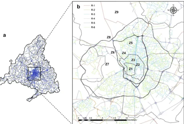
The main source of the information used to feed both HBEFA and COPERT was the traffic model of the Municipality of Madrid. It is a macroscopic simulation model for dynamic equilibrium traffic assignment supported by a Geographic Information System (GIS) where the road network of the metropolitan area of Madrid is represented by 14 938 links. Each of these road segments falls in any of the 9 management areas shown in Fig. 1. Traffic flows and average hourly speeds were available at link level while fleet composition has been estimated at management area level. Traffic flow information is day-specific and vehicle type-specific. This allows taking into account the different temporal activity patterns of each kind of vehicle, an important factor in order to provide an accurate description of air quality (Lindhjem et al., 2012).
Fig. 1. Road network of the traffic model (a) and zoom to the city centre with indication of management areas (b), referred to as Zl—Z9 with distribution of road types in the modelling domain. Rl: Motorway-National (895.1 km); R2: Motorway-City (282.8 km); R3: Trunkroad/Primary-City (771.0 km); R4: Distributor/Secondary (345.5 km); R5: Local/ Collector (477.0 km); R6: Access Residential (795.7 km).
2.3. Implementation of emission models
Emissions for each vehicle type (passenger cars, light duty vehicle, heavy duty vehicles, buses, motorcycles and mopeds) have been calculated according to the vehicle fleet of Madrid for the year 2007. In both cases, emissions have been computed at link level. Subsequent spatial allocation of emissions in the Eulerian grid for air quality modelling is carried out by overlapping (e.g. Borge et al., 2008a).
2.3.2. COPERT
COPERT is an "average speed" model, meaning that calculations rely on speed-dependent equations, which are characteristic of a given vehicle type. Aggregated emission equations were derived for the characteristic vehicle mix of the 9 management areas by weighting factors according to the type of vehicle under two driving situations, urban and motorway. The rural driving pattern
does not occur in the domain of interest. Hourly emissions were computed for each link considering the specific hourly average speed and fleet composition. It should be noted that average speed used is computed in the traffic model as an equilibrium over a number of nodes connecting several links and therefore it may be representative of the average speed concept in an urban driving cycle. Zachariadis and Samaras (1997) and Moussiopoulos et al. (1996) have shown that the COPERT methodology can be used with a sufficient degree of certainty at such high resolution, i.e. for the compilation of urban emission inventories with a spatial resolution of 1 x 1 km2 and a temporal resolution of 1 h (Ntziachristos and Samaras, 2012).
2.3.2. HBEFA
Traffic situation models such as HBEFA, estimate emission factors from a given traffic situation (combination of road type, speed limit and service level) and vehicle type. Consequently,
3 6.1%
2.7% • Passenger cars Q 4%
• Bus urban 2.4%
• Mopeds
D Wbtocycles
O Light duty vehicles a Heavy duty vehicles
D Petrol passenger cars
• Qesel passenger cars
Re-euro Euro 1 Euro 2 Euro 3 Euro 4
a proper definition of the traffic situations that actually occur in Madrid must be made for every link throughout the day. Each link has been assigned to a given road type considering characteristics such as road capacity, number of lanes and free flow speed. As a result, streets and roads from the Madrid traffic model were mapped into six HBEFA road types, according to their generic description. The classification made according to HBEFA road types across the modelling domain is depicted in Fig. 1. Once the road type has been defined, a speed limit was assigned to each link, attending to the free flow speed according to the traffic model. This model includes hourly speed and flow data, but no information on service level (free flow, heavy, saturated and stop & go according to HBEFA) is available. In order to estimate this critical parameter, the HBEFA database was used. The service level of a road was deter-mined from a group of ratios specifically defined to carry out this classification. These ratios measure the relation that exists between the road speed limit and the mean circulation speed. A series of theoretical ratios were obtained using the statistic speeds and speed limits reported by the HBEFA methodology to further cate-gorise the local data available for Madrid (Table 1). Although these statistic speeds are different for every vehicle type, the statistical values for passenger cars were used. This assumption seems reasonable due to the preponderance of such vehicles in the total fleet (Fig. 2). A similar procedure was conducted to estimate the ratios from the information provided by the Madrid traffic model, using, in this case, the average speed and the free flow speed for each link and hour interval (average speed/speed limit) for each link and hour interval. The definition of the service levels was ob-tained by allocating each computed ratio (average speed/speed limit) in the corresponding interval of theoretical ratios embedded in HBEFA for a given road type.
The procedure described yielded a total of 43 different traffic situations (Table 2), which allows obtaining the associated emission factors from the HBEFA database. Consequently, up to 4171 emis-sion factors were obtained in this case study for N0X and NO2
Table 1
Ratios used to assign a level of service.
Road type Level of service Speeda/speed limit
a Speed refers to 1-h average speed according to the traffic model for a particular link.
Table 2
Traffic situations for the Madrid area. Traffic situation ID 1 5 6 9 13 17 21 25 29 33 37 41 2 7 10 14 18 22 26 30 34 38 42 3 8 11 15 19 23 27 31 35 39 43 4 12 16 20 24 28 32 36 40 Level of service Freeflow Heavy Saturated
Stop & go
Road type — Speed limit (km f r1) R 6 - 3 0 R 4 - 5 0 R 4 - 6 0 R 4 - 7 0 R 4 - 8 0 R 5 - 5 0 R 2 - 7 0 R 2 - 9 0 Rl - 100 Rl - 120 R 3 - 5 0 R 3 - 8 0 R 6 - 3 0 R 4 - 6 0 R 4 - 7 0 R 4 - 8 0 R 5 - 5 0 R 2 - 7 0 R 2 - 9 0 Rl - 100 Rl - 120 R 3 - 5 0 R 3 - 8 0 R 6 - 3 0 R 4 - 6 0 R 4 - 7 0 R 4 - 8 0 R 5 - 5 0 R 2 - 7 0 R 2 - 9 0 Rl - 100 Rl - 120 R 3 - 5 0 R 3 - 8 0 R 6 - 3 0 R 4 - 7 0 R 4 - 8 0 R 5 - 5 0 R 2 - 7 0 R 2 - 9 0 Rl - 100 Rl - 120 R 3 - 5 0
Vehicle-0.082 0.017 0.225 0.866 3.368 4.338 3.863 1.999 9.192 24.650 2.286 1.070 0.839 0.035 0.163 0.284 0.623 1.996 1.372 9.049 6.081 3.451 0.729 2.415 0.034 0.096 0.074 0.367 1.367 0.094 2.166 1.398 9.305 0.296 2.633 0.020 0.016 0.085 0.013 0.002 0.113 0.596 2.332
respectively (corresponding to 43 traffic situations times 97 combinations of vehicle type, engine size, fuel and technology). Individual emission factors were then weighted based on the number of vehicles and their respective travelled distance. Emis-sion factors for vehicle categories not available in the HBEFA database (biodiesel, CNG) were taken from COPERT IV. Hourly emissions were obtained from these emission factors through their multiplication by vehicles intensity and link length for every road section and interval.
2.4. Other sectors
Although emissions are dominated by road traffic in Madrid, urban air quality is influenced by a variety of activities (Borge et al., 2012). Table 3 summarizes emissions estimates in the modelling domain for sources other than road traffic. Industrial combustion processes (SNAP 03) are the main NOx emitters (excluding road traffic), although source apportionment studies point out that domestic and residential combustion (SNAP 02) is more relevant for urban air quality in the city centre since industrial sources are located in the surroundings of the Madrid urban area and their emissions are released through relatively high stacks. Similarly, Motorway-National (Rl) Motorway-City (R2) Trunkroad/Primary-City (R3) Distributor/secondary (R4) Local/collector (R5) Access-residential (R6) Freeflow Heavy Saturated Stop + go Freeflow Heavy Saturated Stop + go Freeflow Heavy Saturated Stop + go Freeflow Heavy Saturated Stop + go Freeflow Heavy Saturated Stop + go Freeflow Heavy Saturated Stop + go
Table 3
Summary of emissions (SNAP group level) in the modelling domain excluding road traffic.
SNAP group
01 02 03 04 05 06 08 09 10 11
Total
CO
225
10 004 2238 1083
0 0
2711
441 357 32
17 091
NH3
0 0 0 130 15 212 0
2036 1543
605
4541
NOx
243
3680 10 689
108 0 0
4171 1769
56 125
20 841 PM1 0
50 520 265 51 0 0 360 26 90 0
1362 PM2 5
29 410 210 32 0 0 360 26 13 0
1080
S02
1128 2731 2494
70 0 0 287 6 0 0
6716
VOC
1
1104 1217 3782 2056 48 828
769
5267
17
4682 67 723
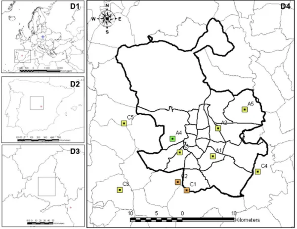
Sparse Matrix Operator Kernel Emissions (SMOKE) modelling system (Borge et al., 2008a; Institute for the Environment, 2009). The meteorological fields needed to simulate air pollution processes have been generated with the Weather Research and Forecasting (WRF) modelling system (Borge et al., 2008b; Skamarock and Klemp, 2008). The modelling domain in this study broadly corresponds to the metropolitan area of Madrid and surroundings and consists of a rectangle with 40 columns and 44 rows with 1 km2 resolution (D4 in Fig. 3). The vertical structure of the model includes 30 layers covering the whole troposphere. Hourly chemical boundary conditions for the annual simulation (year 2007) are obtained from a nested simulation (4 domains) starting from a 48 km resolution domain covering the whole Europe (Dl in Fig. 3). Further details regarding atmospheric processes representation (chemistry, advection, etc.) and model setup can be found in Borge et al. (2010).
most of the emissions from non-road mobile sources (SNAP 08) correspond to the Madrid-Barajas airport and have a very limited impact on urban air quality levels. This emission data set has been considered to simulate air quality levels over Madrid in both model runs, so changes on predicted air quality can be exclusively attrib-uted to the road traffic emission inventory used (COPERTor HBEFA).
2.5. Air quality modelling system and setup
The air quality modelling system (AQM) used is based on the Community Multiscale Air Quality (CMAQ) model (Byun and Ching, 1999; Byun and Schere, 2006). Emissions are processed by the
2.6. Evaluation methodology and observational dataseis
The evaluation of road traffic emission models is not a trivial task. Smit et al. (2010) present a thorough review of recent vali-dation efforts to understand the accuracy and reliability of different emission models. One of the validation methods consists of the comparison of measured ambient pollutant concentrations with the results from combined emission and dispersion modelling. The application of this method may be limited by the assumptions made in the modelling system or the number of locations evalu-ated. Observed NO2 concentration values are available at 34 air quality monitoring stations across the modelling domain (from the
Fig. 3. Air quality modelling domains. The colour squares represent the location of air quality monitoring stations used for evaluation purposes in the 1 km2 resolution modelling
Table 4
N0X and N02 emissions by vehicle type according to COPERT and HBEFA. Vehicle type NOv NO,
Passenger car Light duty
vehicles Heavy duty
vehicles Bus urban Mopeds Motorcycles Taxis Total
COPERT 9904 1504
10 803
4495 24 105 1125 27 961
HBEFA 11 933
2084
12 406
5784 6 268 1318 33 799
Diff. (%) 20.5 38.6
14.8
28.7 -74.0 154.9 17.1 20.9
COPERT 3086
469
1415
554 0 0 420 5944
HBEFA 3411
647
1346
821 0 14 477 6718
Diff. (%) 10.5 38.0
-4.8
48.3 -13.6 13.0
(RMSE), Mean Bias (MB) and correlation coefficient (r) are shown in the results section, since this minimum group of statistics provides a meaningful summary of model performance. These statistics are given in Equations (1)—(3) respectively, where N is the total number of pairs of observed—modelled values (up to 8760 for a particular monitoring station). P, O represent the mean of the predicted and observed series respectively.
1
M B = Ñ E (P¡ -0¡ )
RMSE =
¡ = 1
\
1 N
( i )
(2)
i = l
Madrid City Council and Madrid Greater Region air quality moni-toring networks). However, the evaluation of an air quality model through comparison with observations requires a consistency between the representativeness of the observational datasets (time and space scales) and the temporal and spatial scales of the air quality model. Considering the model resolution (1 h, 1 km2) and data availability, 10 monitoring stations distributed throughout the modelling domain (Fig. 3) have been selected to support the air quality model evaluation and thus the assessment of the emission inventories being compared. This selection includes mostly back-ground urban locations, which is also consistent with the purposes of the study since urban background levels in Madrid are domi-nated by road traffic (Borge et al., 2012).
Although this methodology has little discriminating power to understand model behaviour, it is generally recognised that domain-wide statistics based on the comparison of observed and modelled concentration values may provide a general performance measure on the capability of the model to replicate observed values. Considering that the only difference between the two model runs compared consists of the road traffic emission inven-tory (i.e. emissions from other sources, boundary conditions, meteorology, etc. are kept constant), it is assumed that model performance can be used to assess the goodness of both estimates (COPERT and HBEFA). In order to determine which of the calcula-tion methods fits best with the observacalcula-tions, a series of common statistics have been calculated for each monitoring station using pairs of observed (O,) and predicted (P,) ambient concentration values with 1 h resolution (Borrego et al., 2008; Borge et al., 2010). However, only the results in terms of Root Mean Square Error
E f = i ( P i - P ) - O i - o
^lÁPi-pf-^lÁOi-of
(3)
3. Results
This section presents and compares the emission resulting from the application of the COPERT and HBEFA models in the modelling domain as well as the statistical analysis of the corresponding air quality simulations carried out. As stated in the introductory section, the discussion and analysis is focused on NOx and most particularly on NO2.
3.1. Emissions
In general, the resulting emissions obtained with the HBEFA emission calculation model are higher than those computed with COPERT (Table 4). NOx emissions in the modelling domain are 33 799 and 27 961 tons respectively, i.e. total emissions from HBEFA are 20.9% higher. According to these estimates, NOx emissions from road traffic would exceed the sum of the rest of emitting sectors (Table 3) in a 34% and 62% respectively. Thus, road traffic would be responsible for 57.3% and 61.9% of total NOx emissions in the modelling domain depending on the road traffic model used. The spatial distribution of the NOx emissions yielded by both compu-tation methods is shown in Fig. 4.
For the specific case of NO2, the emissions estimated by HBEFA are only a 13.0% higher if compared to COPERT (Table 5) since
Table 5
Summary statistic evaluation of modelled N02. MB
-square error, r — correlation coefficient.
mean bias; RMSE — root mean
Monitoring station Al A2 A3 A4 A5 CI C2 C3 C4 C5 Total N 8749 8733 8753 8718 8751 8686 8721 8685 8730 8695 87 221
MB (|ig m
COPERT 1.9 - 2 . 6 - 1 0 . 3 - 9 . 1 - 5 . 4 - 0 . 4 5.2 - 6 . 4 - 1 . 3 1.1 - 2 . 7
-
3)
HBEFA 6.9 2.0 - 5 . 6 - 5 . 4 -1.7 4.8 9.9 - 1 . 4 3.6 5.8 1.9
RMSE(ngirr3)
COPERT 32.2 26.8 31.3 26.8 27.8 32.1 33.0 25.3 21.8 22.4 28.0 HBEFA 34.6 28.6 31.7 27.2 29.0 33.7 35.0 25.9 24.0 25.2 29.5 r (dimensi COPERT 0.598 0.574 0.563 0.584 0.534 0.709 0.691 0.751 0.654 0.641 0.630 onless) HBEFA 0.601 0.580 0.571 0.589 0.541 0.706 0.696 0.755 0.665 0.646 0.635
resulting average NC^/NOx ratios are lower for HBEFA (0.199 vs 0.213). Although N02/NOx ratios considered in HBEFA are higher for some vehicle categories (e.g. diesel passenger car Euro3, petrol passenger car Euro 4 or heavy duty vehicles Euro 4), the global speciation of NOx is strongly influenced by Euro 4 diesel passenger cars (primary N02 ratio of 0.55 and 0.40 in COPERT and HBEFA respectively).
A detailed comparison between the COPERT and HBEFA results reveals that the differences in the estimation of NOx emissions are mainly related to passenger cars, heavy duty vehicles and buses (Table 4). NOx emissions from passenger cars according to HBEFA are 20.5% higher than those estimated by COPERT. Considering the distribution of travelled distance by vehicle type in Madrid (Fig. 2a) this accounts for 34.8% of the difference between total NOx emis-sions from road traffic. Although urban buses and heavy duty vehicles represent less than 10% of total mileage, they are respon-sible for 49.5% of the departure of total NOx estimates. This is due to a large discrepancy in the emission factors assigned to these vehicle types that may be explained by the implicit consideration of rather different speeds or dissimilar flow conditions.
As for NO2, important differences have been found mainly for passenger cars and buses (Table 4). Although the deviation between models in the estimation of NO2 emissions for passenger cars is smaller than for NOx, it still represents 42.1% of the total difference in NO2 emissions for the whole sector. NO2 emissions computed by
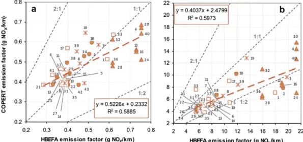
HBEFA are 48.3% higher than those of COPERT which represents 34.6% of total difference between the two models compared for this pollutant. These discrepancies may be attributed basically to the difference in emission factors assigned for traffic situations where the service level is stop & go (represented by triangles in Fig. 5). The analysis of the frequency in which a vehicle circulates under each of the 43 traffic situations in Madrid points out that the stop & go service level is relatively common (Table 2). Although this service level represents less than 6% of total vehicle-km, this figure reaches a 24% in the centremost part of the studied domain. The relative difference in the emission factors for passenger cars under this traffic situation is 13%. The observed difference between models may be directly influenced by the methodology used to assign an emission factor from HBEFA. According to the methodology implemented, a road or street is associated to a traffic condition and then the corresponding emission factor from the HBEFA database is selected. However, this emission factor may not be necessarily representative of the average speed of a particular link. Therefore, it is interesting to investigate the response of the COPERT model when applied to the statistical speeds embedded in HBEFA emis-sion factors. This analysis is useful to discriminate whether errors may arise from the HBEFA implementation carried out more than intrinsic differences between emission models.
3.2.2. Influence of average speed
In order to study the influence of this issue in the results, an average speed has been calculated considering links with the same traffic situation. The obtained average speeds were compared then with the statistical speed of the corresponding situations in HBEFA for every traffic situation and vehicle type. Fig. 6 illustrates the comparison of average speeds used in COPERT with those implicitly considered in HBEFA. The graph represents the resulting average for each service level (weighted by the share of Vehicle-km shown in Table 2). It can be seen that average speeds used to compute emis-sions in COPERT fairly correspond to those statistical speeds implicit in HBEFA for passenger cars. Implicit HBEFA speed is 3.4%, 2.7% and 13.9% higher for free flow and heavy situations respectively. Oppo-sitely, average HBEFA implicit speed for the stop & go service level is 17,5% lower than the corresponding average speed used to feed COPERT. Global weighted average speeds differ only in a 4.1%. A similar situation (not shown) has been found for light vehicles.
As for urban buses, significant discrepancies are found for all the service levels. In this case, implicit HBEFA speeds are systematically
E
I
DÉ UJ a. O o 0.8 0.7 0.6 • - 0.5 0.4 0.3 0.2a 2 : 1 /
s
X
Á
4 5
e
\ A »
¡¡to-4iNÉK¿9<,'
2 1
G r ^ / x J
2 2» *
I'M»-/ 11 .
27u
-• ' 1 f 1 IS
t
,'
*
D.4'3¿ 3 2
Xy' S
•"" i d .36
i
2
8— 5
v.y''
A 40
12
A 24
' ' ' l : 2 y = 0.5226X + 0.2332
(¥ = 0.5885
0.2 0.3 0.4 0.5 0-6 0.7
HBEFA emission factor (g NOx/km) 0 8 22 20 18 16 14 12 10 8 6 4 2
y = 0.4037X + 2.4799 ^ = 0.5973
f ^ , ' l l
267
'• 1
1
/
t t / i2 : 1 / '
/ 11
1:1 , " '
/
A .
A
»
/
D
V
9
^ \?'
%
" ' " " \
LD 5 1:2 28
^ ^ , , — Ü - , , , ,
b
/
4-] 2
1
, ' '
2 0 A 4A «A <*--3- «
A 244 6 8 10 12 14 16 18 20 22
HBEFA emission factor (g NOx/krn)
Freeflow Heavy Saturated Stop & go
Traffic s i t u a t i o n
• Traffic mpdel average speed (used for COPERT) •Average HBEFA statistical speed (passenger cars) •Average HBEFA statistical speed (urban buses)
Fig. 6. Comparison between the average speeds used in COPERT (traffic model) and
the corresponding statistical speeds considered by HBEFA for the emission factors applied to Madrid (passenger cars and urban buses).
lower than those used for COPERT, particularly for the stop & go service level (28,4%). Differences are also remarkable for coaches and heavy duty vehicles, which exhibit very high relative NOx emission factors and thus have a strong impact on the global emission estimation. The reason for this disagreement may be ultimately related to the criteria used to assign a service level, since the speed/limit speed ratios used for this purpose were derived from passenger cars statistical data.
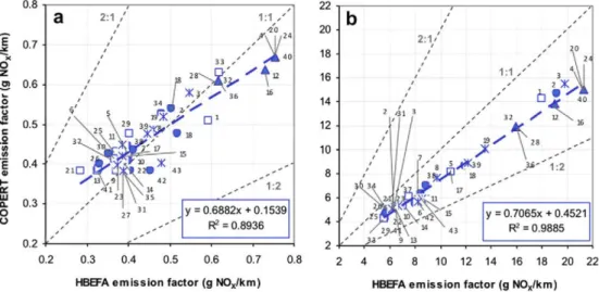
Once the differences between the two possible speed types have been made evident, the COPERT equations were fed with the statistical speeds obtained from HBEFA in order to remove the influence of speed from the differences. This analysis allows a more consistent comparison between the emission factors implemented in both computation models. In general, for all types of vehicles, the values of the resulting emission factors obtained (Fig. 7) approach to those specified by HBEFA. The spread of the scatter plot decreases considerably, especially for urban buses (the determi-nation coefficient, r2, increases from 0.597 to 0.988) although HBEFA emission factors remain higher than those from COPERT. It can be observed in Fig. 7b how HBEFA emission factors for urban buses are a 31.9% higher than those resulting from COPERT for the same average speeds. The relation between emission factors for the Madrid average passenger car is not so clear. As illustrated in Fig. 7a,
emission factors from COPERT tend to be higher than those of HBEFA at medium and high speeds.
3.2. Ambient air quality levels
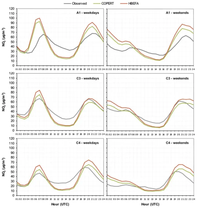
The emissions of both models discussed in Section 3.1 were processed and fed to CMAQ to run the year 2007. The results are illustrated through the NO2 annual mean concentration in Fig. 8. As expected, predicted ambient air quality levels present a very similar spatial pattern but are higher when the chemical-transport model is fed with the emission estimates from HBEFA. The comparison of these results with observed values in representative monitoring stations is summarized in Table 5.
The model slightly underestimates NO2 concentrations overall when fed with COPERT emissions (global mean bias of -2.7 |ig mr3). On the contrary, HBEFA emissions turn out in an aggregated overestimation of 1.9 |ig irT3. This may indicate that actual emissions from road traffic may be in between those esti-mated by COPERT and HBEFA. However, absolute errors (repre-sented in Table 5 by the RMSE) related to the HBEFA run (29.5 |ig irT3) are slightly larger than those of COPERT (28.0 |ig irT3), suggesting that HBEFA emissions may be over-estimated. Nevertheless, HBEFA yielded a slight but consistent improvement of the correlation coefficient (r) for all the locations included in the analysis. Average daily concentration profiles were examined in order to achieve a better understanding of the model behaviour and the reason for discrepancies between the two inventories compared. As illustrated in Fig. 9, CMAQ predicts reasonably well the typical NO2 concentration patterns, both for working and non-working days. There are locations (such as station Al) where both traffic inventories cause the chemical-transport model to overestimate observed values. C3 is a location represen-tative of the opposite situation, i.e. both model runs present an overall underestimation of observed concentration values. Results for C4 are shown as representative of the average model behaviour over the whole modelling domain. It can be seen that in all cases, CMAQ predictions corresponding to the HBEFA emission estimate are above those of COPERT, mainly in the peak hours of the day, where congestion is more frequent, indicating that HBEFA may be overestimating actual emissions for those traffic situations. These results, in fact, may support the conclusions of Smit et al. (2010) that suggested that both, average-speed and traffic-situation models, may overestimate NOx emissions, at least for high traffic
s
a.
HI
0-O ü
40 A i/24
X i ' V
3 6A»
«S^
Q1
0.3 0.4 0.5 0.6 0.7
HBEJ-A emission factor (g NUx.'km)
4 6 8 10 12 14 16 18 20 22
HBEFA em iss ion factor (g NOx/km)
Fig. 7. Comparison of average emission factors for representative vehicles in this study (passenger cars, a and urban buses, b) for the 43 traffic situations found in Madrid when
íígrrv1
100
90
80
70
60
50
40
30
20
10
0
u
\
\
km.
A1
^ s a — - ^
A1 - weekends
y *
S s a ^ ^ /
0 1 0 2 0 3 0 4 0 5 0 6 0 7 0 8 0 9 10 1112 13 14 1 5 1 6 17 13 19 2 0 2 1 2 2 7 ) 24 0 ! Oí Oí 04 0 5 0 6 07 OS 09 10 1 1 1 2 1 3 14 1 5 1 5 17 18 19 2 0 2 1 2 2 2 3 2 4
Fig. 8. Predicted N02 annual mean (|ig m 3) concentration by CMAQwhen fed with emission datasets from COPERT (a) and HBEFA (b).
Observed COPERT HBEFA 120
110 100
90
80 70
60 50
40 30
20 10
0
120
110
100
90
80
70
60
50
40 30
20
10 0
120 110
100
90 80
70
60
50 40
30 20
10
0
0 1 0 2 0 3 0 4 0 5 0 6 0 7 0 8 0 9 10 11 12 13 14 15 16 17 18 B 2 0 2 1 22 2 3 2 4 0 1 0 2 03 0 4 05 0 6 0 7 0 8 0 9 10 11 12 13 14 15 16 17 16 19 2 0 2 1 2 2 2 3 24
Hour (UTC) Hour (UTC)
-V
^ s s s </
C3 - weekends
\>^ y*
V
0 1 0 2 0 3 0 4 0 5 0 6 0 7 0 8 0 9 10 11 12 13 M 15 15 17 1 S 1 9 2 0 2 1 2 2 2 3 2 4 o i 0 2 O 3 O 4 O S O 6 O 7 O 8 O S JQ 11 12 13 14 15 16 17 13 19 2 0 2 1 2 2 23-24
C4
.
C4
intensities. The discrepancies however are strongly influenced in both cases by the input data, since it is clear that emissions in the afternoon are underestimated. This underestimation compensates to a certain extent the overestimation during the peak hours. It is observed that the model exhibits a better behaviour over the weekends, probably because traffic patterns for non working days present less variability than those corresponding to the different weekdays.
4. Conclusions
According to the results of this study, road traffic is the main responsible for NOx emissions in Madrid, exceeding all other sectors together. Among mobile sources, passenger cars, heavy duty vehicles and buses are the main emitting sources of NO2. Each vehicle category has a different relevance depending on the ana-lysed urban area, being emissions from passenger cars higher at centremost areas. Oppositely emissions from heavy duty vehicles and buses concentrate in areas far from the city centre.
The comparison between the results of the two models imple-mented indicates that the emissions obtained from HBEFA are higher than those corresponding to COPERT, namely a 20.9% in the case of NOx and 13.0% for NO2. The differences in these percentages are strongly affected by discrepancies on low-speed traffic situa-tions, more specifically under the stop & go service level, relatively frequent in Madrid (approximately 6% of total vehicle-km in the whole domain and 24% in the city centre).
A significant difference between methodologies is the consid-eration of speed. The inventory compiled with the COPERT model uses the average speed of a particular link regardless of the type of vehicle (a limitation of the traffic model), while the HBEFA meth-odology provides statistic speeds for different vehicle types under every traffic situation.
From the results of this case study it may be inferred that the observed differences are related to intrinsic differences of the emission factors used but also to the procedure used to represent traffic conditions (underlying average speed).
The emission factors reported by HBEFA correspond to different driving patterns of particular countries which might not reflect the traffic reality of Madrid. It can be generally concluded that the emission factors included in this database might not be represen-tative of the particular conditions of other countries and a throughout analysis for their implementation is required.
In order to gain some understanding regarding the accuracy and reliability of both estimates, the resulting emissions were used to simulate air quality levels over Madrid and further compared with observations from the monitoring networks available in the modelling domain. It was found that the CMAQ chemical-transport model yielded low biases for NO2 in both cases. Although emission factors from HBEFA are presumably more representative of real traffic emissions, the comparison of the observed and modelled ambient air NO2 levels in this case study indicates that COPERT may be providing more realistic emission estimates, since this option yields lower errors, yet it presents slightly lower correlation coef-ficients. HBEFA emission estimates bring about lower global biases, although it is mostly due to error compensation (overestimation in the peak hours and underestimation in the afternoon). However, the analysis of the causes for emission discrepancies between both emission computation approaches points out that errors cannot be attributed only to the models themselves but also to the imple-mentation methodology and limitations related to the input data-sets. Therefore, in order to minimize errors in the road traffic emission inventory, a series of improvements regarding activity data should be implemented. Although the results from this study may be contrasted and generalized with further experiments, the
most effective options to improve the application of road traffic models in Madrid may include the following:
- Considering that the observed discrepancies between models are higher for stop & go traffic situations, it would be inter-esting to investigate new classification criteria for each of the service levels. This is evidenced by the fact that the road speed limit/mean circulation speed ratio used in the method is very high for dense traffic situations, i.e. stop & go service levels. A possible alternative method to classify the service level would be the use of a parameter that measures the intensity of vehicles across a given link against the capacity of the road/ street. This parameter should be evaluated in terms of its dependency with speed, where sharp changes would mark the boundaries between the different service levels.
- To incorporate vehicle type-specific average speeds in the traffic model. This is particularly important for those vehicles with very high emission factors usually running at low speed. According to this study, the difference of average speed implicit in the HBEFA emission factors used for urban buses and the speed in the traffic model reaches a -25% as an average. Therefore it is highly recommendable that, at least, buses should be treated separately concerning speed. Otherwise HBEFA emission factors may be inaccurately assigned bringing about important errors.
Acknowledgements
The Madrid city Council provided the traffic model and partially supported this study. The CMAQ modelling system was made available by the US EPA and it is supported by the Community Modeling and Analysis System (CMAS) Center. The authors also acknowledge the use of emission datasets and monitoring data from the Dirección General de Calidad y Evaluación Ambiental of the MARM and the Portuguese Ministry of Environment. Comments and suggestions from peer reviewers are also acknowledged.
References
Ayuntamiento de Madrid (AM), 2010. Inventario de emisiones de contaminantes a la atmósfera en el Término Municipal de Madrid. Prepared by AED for the Madrid City Council. D.G. de Calidad, Control y Evaluación Ambiental. Servicio de Calidad del Aire.
Bishop, G.A., Peddle, A.M., Stedman, D.H., 2010. On road emission measurements of reactive nitrogen compounds from 3 Californian cities. Environmental Science & Technology 44, 3616-3620.
Borge, R., Lumbreras, J., Rodriguez, E., 2008a. Development of a high-resolution emission inventory for Spain using the SMOKE modelling system: a case study for the years 2000 and 2010. Environmental Modelling & Software 23, 1026-1044.
Borge, R., Alexandrov, V., del Vas, J.J., Lumbreras, J., Rodriguez, E., 2008b. A comprehensive sensitivity analysis of the WRF model for air quality appli-cations over the Iberian Peninsula. Atmospheric Environment 42, 8560—8574. Borge, R., López, J., Lumbreras, J., Narros, A., Rodriguez, E., 2010. Influence of
boundary conditions on CMAQ simulations over the Iberian Peninsula. Atmo-spheric Environment 44, 2681—2695.
Borge, R., Lumbreras, J., Pérez, J., de la Paz, D., Vedrenne, M., Rodriguez, E., 2012. Emission inventories and modeling activities for the development of air quality plans in Madrid (Spain). In: US EPA Annual International Emission Inventory Conference "Emission inventories — Meeting the Challenges Posed by Emerging Global, National, Regional and Local Air Quality Issues", Tampa (Florida), August 13-16, 2012.
Borrego, C, Monteiro, A., Ferreira, J., Miranda, A.I., Costa, A.M., Carvalho, A.C., Lopes, M., 2008. Procedures for estimation of modelling uncertainty in air quality assessment. Environment International 34, 613—620.
Byun, D.W., Ching, J.K.S., 1999. Science Algorithms of the EPA Models-3 Community Multi-scale Air Quality (CMAQ) Modeling System. EPA/600/R-99/030. USEPA National Exposure Research Laboratory, Research Triangle Park, NC.
Carslaw, D.C., Beevers, S.D., Tate, J.E., Westmoreland, E.J., Williams, M.L., 2011. Recent evidence concerning higher NOx emissions from passenger cars and light duty vehicles. Atmospheric Environment 45, 7053—7063.
European Environment Agency (EEA), 2011a. European Union Emission Inventory Report 1990—2009 under the UNECE Convention on Long-range Transboundary Air Pollution (LRTAP). EEA Technical Report No 9/2011, ISBN 978-92-9213-216-3. Available online at: http://www.eea.europa.eu/publications/eu-emission-inventory-report-1990-2009.
European Environment Agency (EEA), 2011b. Air Quality in Europe — 2011 Report. EEA Technical Report No 12/2011, ISBN 978-92-9213-232-3. Available online at:
http://www.eea.europa.eu/publications/air-quality-in-europe-2011.
Grice, S., Stedman, J., Kent, A., Hobson, M., Norris, J., Abbott, J., Cooke, S., 2009. Recent trends and projections of primary N02 emissions in Europe. Atmo-spheric Environment 43, 2154—2167.
Haan, P. de, Keller, M., 2000. Emission factors for passenger cars: application of instantaneous emission modelling. Atmospheric Environment 42, 916—926. Hanna, S.R., 2007. In: Borrego, C, Renner, E. (Eds.), A Review of Uncertainty and
Sensitivity Analyses of Atmospheric Transport and Dispersion Models. Developments in Environmental Science, vol. 6. Elsevier Ltd., pp. 331—352 (Chapter 4).
Hausberger, S., Rexeis, M., Zallinger, M., Luz, R., 2009. Emission Factors from the Model PHEM for the HBEFA Version 3. Graz University of Technology, Institute for Internal Combustion Engines and Thermodynamics. Report Nr. 1-20/2009 Haus-Em 33/08/679 from 07.12.2009.
HBEFA, 2010. Handbuch Emissionsfaktoren des Strassenverkehrs 3.1 — Doku-mentation. Infras, UBA, Berlin. BUWAL, Bern/UBA, Wien. Available from: www.
hbefa.net.
Institute for the Environment, 2009. SMOKE v2.6 User's Manual. University of North Carolina, Chapel Hill, NC. Available online at: http://www.smoke-model.org/
version2.7/html/ch01.html (accessed 30.01.11).
Kioutsioukis, L, Kouridis, C, Gkatzoflias, D., Dilara, P., Ntziachristos, L, 2010. Uncertainty and sensitivity analysis of national road transport inventories compiled with COPERT 4. Procedía — Social and Behavioral Sciences 2, 7690— 7691.
Kioutsioukis, L, Tarantela, S., Saltelli, A., Gatelli, D., 2004. Uncertainty and global sensitivity analysis of road transport emission estimates. Atmospheric Envi-ronment 38, 6609-6620.
Kousoulidou, M., Ntziachristos, L, Mellios, G., Samaras, Z., 2008. Road-transport emission projections to 2020 in European urban environments. Atmospheric Environment 42, 7465-7475.
Lindhjem, C.E., Pollack, A.K., DenBleyker, A., Shaw, S.L, 2012. Effects of improved spatial and temporal modeling of on-road vehicle emissions. Journal of the Air & Waste Management Association 62, A7X-A7&.
Lumbreras, J., Valdés, M., Borge, R., Rodriguez, M.E., 2008. Assessment of vehicle emissions projections in Madrid (Spain) from 2004 to 2012 considering several control strategies. Transportation Research, Part A 42, 646—658.
Moussiopoulos, N., Sahm, P., Papalexiou, S., Samaras, Z., Tsilingiridis, G., 1996. The Importance of Using Accurate Emission Input Data for Performing Reliable Air Quality Simulations. Eurotrac Annual Report. Computational Mechanics Publi-cations, pp. 655—659.
Ntziachristos, L, Gkatzoflias, D., Kouridis, C, Samaras, Z., 2009. COPERT: a European road transport emission inventory model. In: Athanasiadis, I.N., Mitkas, PA, Rizzoli, A.E., Marx Gómez, J. (Eds.), Information Technologies in Environmental Engineering. Springer, pp. 491—504.
Ntziachristos, L, Samaras, Z., 2012. Methodology for the Calculation of Exhaust Emissions - SNAPS 070100-070500, NFRs lA3bi-iv (EMEP/CORINAIR 2009 Atmospheric Emissions Inventory Guidebook chapter, updated May 2012). Available at: http://www.eea.europa.eu/publications/emep-eea-emission- inventory-guidebook-2009/part-b-sectoral-guidance-chapters/l-energy/l-a-combustion/I.a3.b-road-transport-gb2009-update.pdf.
Pujadas, M., Nunez, L, Plaza, J., Bezares, J.C., Fernández, J.M., 2004. Comparison between experimental and calculated vehicle idle emission factors for Madrid fleet. Science of the Total Environment 334—335,133—140.
Rexeis, M., Hausberger, S., 2009. Trend of vehicle emission levels until 2020 — prognosis based on current vehicle measurements and future emission legis-lation. Atmospheric Environment 43, 4689—4698.
Skamarock, W.C, Klemp, J.B., 2008. A time-split nonhydrostatic atmospheric model. Journal of Computational Physics 227, 3465—3485.
Smit, R., Bluett, J., 2011. A new method to compare vehicle emissions measured by remote sensing and laboratory testing: high-emitters and potential implica-tions for emission inventories. Science of the Total Environment 409, 2626— 2634.
Smit, R., Brown, A.L., Chan, Y.C., 2008. Do air pollution emissions and fuel consumption models for roadways include the effects of congestion in the roadway traffic flow? Environmental Modelling & Software 23,1262—1270. Smit, R., Ntziachristos, L., Boulter, P., 2010. Validation of road vehicle and traffic
emission models — a review and meta-analysis. Atmospheric Environment 44, 2943-2953.
Smit, R., Poelman, M., Schrijver, J., 2007. Improved road traffic emission inventories by adding mean speed distributions. Atmospheric Environment 34,4629—4638. Swall, J.L, Foley, K.M., 2009. The impact of spatial correlation and
incommensura-bility on model evaluation. Atmospheric Environment 43,1204—1217. Velders, G.J.M., Geilenkirchen, G.P., de Lange, R., 2011. Higher than expected NOx
emission from trucks may affect attainability of N02 limit values in the Netherlands. Atmospheric Environment 45, 3025—3033.
Williams, M.L., Carslaw, D.C., 2011. New directions: science and policy — out of step on NOx and N02. Atmospheric Environment 45, 3911-3912.
Winiwarter, W, Kuhlbusch, T.A.J., Viana, M., Hitzenberger, R, 2010. Quality considerations of European PM emission inventories. Atmospheric Environ-ment 43, 3819-3828.