Reduction of truncation errors in planar, cylindrical and partial spherical near-field antenna measurements

(1)

Volume 2012, Article ID 438727,19pages doi:10.1155/2012/438727

Research Article

Reduction of Truncation Errors in Planar, Cylindrical, and

Partial Spherical Near-Field Antenna Measurements

Francisco Jos´e Cano-F´acila,

1

_{Sergey Pivnenko,}

2

_{and Manuel Sierra-Casta˜}

_ner

1

1_{Radiation Group, Signals, Systems and Radiocommunications Department, Technical University of Madrid,} Avenue Complutense 30, 28040 Madrid, Spain

2_{Department of Electrical Engineering, Technical University of Denmark, 2800 Kongens, Lyngby, Denmark}

Correspondence should be addressed to Francisco Jos´e Cano-F´acila,[email protected]

Received 12 July 2011; Accepted 8 September 2011

Academic Editor: Claudio Gennarelli

Copyright © 2012 Francisco Jos´e Cano-F´acila et al. This is an open access article distributed under the Creative Commons Attribution License, which permits unrestricted use, distribution, and reproduction in any medium, provided the original work is properly cited.

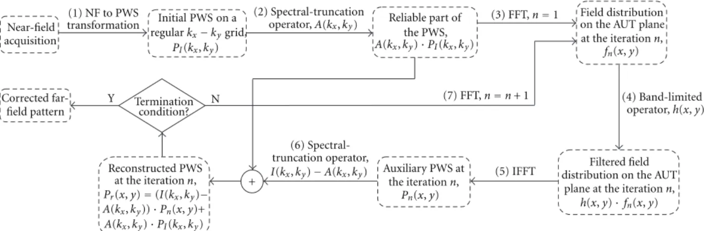
A method to reduce truncation errors in near-field antenna measurements is presented. The method is based on the Gerchberg-Papoulis iterative algorithm used to extrapolate band-limited functions and it is able to extend the valid region of the calculated far-field pattern up to the whole forward hemisphere. The extension of the valid region is achieved by the iterative application of a transformation between two diﬀerent domains. After each transformation, a filtering process that is based on known information at each domain is applied. The first domain is the spectral domain in which the plane wave spectrum (PWS) is reliable only within a known region. The second domain is the field distribution over the antenna under test (AUT) plane in which the desired field is assumed to be concentrated on the antenna aperture. The method can be applied to any scanning geometry, but in this paper, only the planar, cylindrical, and partial spherical near-field measurements are considered. Several simulation and measurement examples are presented to verify the eﬀectiveness of the method.

1. Introduction

In many cases, antenna parameters, such as gain, directivity, radiation pattern, side-lobe level, and beamwidth, cannot be determined directly from measurements that are obtained in a far-field range because the distance to the far-field region may be too large. However, it is well known that those parameters can be obtained using analytical transformations from near-field measurements [1–4]. Moreover, these types of measurement can be performed in indoor ranges, reduc-ing unwanted contributions from the environment, such as reflections or diﬀractions, as much as possible.

One important requirement to determine exact far-field patterns from near-field acquisitions is the ability to measure the electric or magnetic field that is tangential to an arbitrary surface that encloses the antenna under test (AUT). If that condition is satisfied, the field can be obtained anywhere outside the measurement surface and specifically in the far-field region by solving an integral over the surface on which

(2)

the AUT is fully enclosed by the acquisition surface. There-fore, there are no truncation errors in the calculated far-field pattern. In the planar field (PNF) and cylindrical near-field (CNF) measurements, because of the finite size of the scan surface, the closed surface condition is never fulfilled, and, consequently, the true far-field pattern is never known in the whole sphere, that is, the pattern is only valid within the called reliable region. A second eﬀect, which is caused by the discontinuity of the measured field at the edge of the scan surface, is the presence of a ripple within this region.

Because the truncation error is an unavoidable error in PNF and CNF measurements, and it is not present in SNF measurements, most of the approaches to reduce this kind of error have been specifically proposed for the two first configurations. These approaches can be divided into two groups. The first group attempts to reduce the second eﬀect that was mentioned previously, that is, the ripple within the reliable region by the application of proper window functions to the near-field data. In [5,6], a directive synthetic array of probes is created by combining near-field data points to reduce the level at the edges of the measurement plane. This approach provides noticeable ripple reduction, especially for the measurement of low-directive antennas. Another ripple reduction approach is proposed in [7,8] in which raised cosine amplitude and quadratic phase windows are shown to provide high accuracy. Although windowing techniques can greatly reduce erroneous ripples, an extra scan area is needed to obtain the same reliable region. If the scan area is not extended with the use of one of these techniques, the extent of the reliable region is reduced.

The approaches of the second group do not attempt to reduce the ripple within the region in which the far-field pattern is reliable, but they attempt to obtain a good estimation of the true pattern outside of that region. One of these approaches, called the equivalent magnetic current approach [9], presents a method of computing far-fields in the whole forward hemisphere from planar near-field mea-surements. The idea is to compute the equivalent magnetic currents in the AUT plane by solving the system of integral equations that relate these currents and the measured field. Once these currents are known, it is possible to produce the correct far-fields in front of the AUT. The main drawback of this approach is the great computational complexity that is required to solve the system of integral equations. However, that complexity may be drastically reduced by using a mag-netic dipole array approximation instead of the equivalent magnetic current approach, eliminating the numerical inte-gration in the process. Another strategy to reduce truncation errors is to rotate the AUT about one or more axes [10], mea-suring in diﬀerent planes and combining them to increase the maximum validity angle. Logically, this technique requires a particular near-field to far-field transformation for each combination of plane acquisitions. In [11], the problem of truncation is addressed using a priori information about the AUT. The main idea of this approach is to estimate the near-field data outside of the scanning area by extrapolating the measured data before calculating the far-field pattern. The

a priori information is employed to obtain a nonredundant

and nonuniform representation [12] of the samples that are

taken over the measurement surface. Thanks to this distri-bution of the samples, a large amount of samples outside of the scan plane can be recovered with good accuracy. This strategy was experimentally validated in [13], obtaining good far-field results for the case of cylindrical scanning. The same idea of nonredundant and nonuniform representation of electromagnetic fields was also used in [14] for extrapolating the data outside of a plane-polar scanning. In this last work, however, optimal sampling interpolation expansions instead of the cardinal series expansions employed in [11,12] are applied. In [14], it is numerically demonstrated that these new expansions guarantee a better reconstruction of the sam-ples outside the measurement surface for a given number of measurement points. However, these extrapolation methods are not able to remove the truncation error in all the far-field pattern. A new method that is based on the same principle, that is, the use of a nonredundant sampling in the acquisi-tion, was proposed in [15]. In this method, the truncation error is practically eliminated by also addressing points in surfaces external to the actual scanning area. Therefore, this method can be applied whenever the set-up allows the varia-tion of the distance between the AUT and the probe. Another alternative to increase the reliable region by extrapolating the planar near-field data is described in [16]. The extrapolation is achieved by first back-propagating the measured field to the AUT plane. After that, only the samples within the AUT aperture are retained, and they are used to restore the external samples in terms of a diﬀraction integral along the aperture rim. Finally, the field is transformed back to the measurement plane to obtain new field samples outside of the measurement region. The main drawback of this last approach is, as in [11,12,14], the impossibility of recovering samples over an infinite surface with good accuracy, and, therefore, the truncation error is not completely removed for large elevation angles. A recent publication [17] also uses a

priori information about the AUT in an iterative algorithm

(3)

the classical spherical modal functions in the uncompleted surface. Therefore, the calculated modal coefficients are incorrect. This problem can be solved by employing a new basis function set that is orthogonal over the truncated angular domain. It is subsequently necessary to derive a near-field to far-near-field transformation for the resulting coefficients. This solution was presented for two-dimensional cylin-drical/spherical near-field scanning in [21] and for three-dimensional acoustic spherical near-field scanning in [22]. The alternative expansion considered in these works is based on Slepian functions [23]. In some cases, it is not the mea-surement time that is the limitation of SNF meamea-surements, but the impossibility to get reliable data over the whole sphere, for example, due to support-structure blockage when measuring electrically small antennas. In [24], a method that is based on a least-squares technique is employed to calculate the spherical wave coefficients using forward hemisphere data only. This method can significantly reduce truncation errors, but it is not efficient for large antennas. This problem is also addressed in [25] where the band-limited property of the spherical wave coefficients is exploited in an iterative algorithm that substitutes the unreliable portion of the meas-urement sphere with new samples at each iteration.

In the present work, a method to reduce truncation errors when measuring the field overtruncated surfaces is de-veloped. The method is based on the iterative algorithm that was proposed in [18,19], and it has already been applied to the PNF case in [17]. However, this method can be applied to any scanning geometry by taking certain considera-tions into account. Therefore, this work can be viewed as a generalization of the method presented in [17]. Moreover, compared to some aforementioned approaches, it is not nec-essary to take samples in surfaces external to the actual scan-ning area. Therefore the reduction of truncation errors is achieved without increasing the measurement time. In addi-tion, the computational cost is not large because the method is based on the iterative application of Fourier transforms between the plane wave spectrum (PWS) and the extreme near-field, and those transforms can be made quite rapid by using fast fourier transform techniques, not as in [9] where the equivalent magnetic currents are obtained by solving a complex system of integral equations.

A bottleneck of the method presented in [17] may be the time required to find the optimum termination point in the iterative procedure. In this work, a faster procedure based on the Gradient Descent algorithm, with which is possible to obtain the iteration number where the error is minimum, is proposed.

The method provides an exact reconstruction when starting from error free data. In practice, the measured data are always aﬀected by errors, and therefore, the method does not converge to the exact solution. However, the method is very insensitive to errors and is able to provide a very good radiation pattern reconstruction using initial data corrupted by noise or other measurement errors.

The main limitation of the method is that the truncation error can only be removed in the forward hemisphere. More-over, it is within the methods that require a priori informa-tion about the AUT, like all the methods based on a

non-redundant and nonuniform representation of the samples [11–15]. In our case, it is necessary to know exactly the AUT dimensions. Due to this fact, the best results are obtained when the AUT is an aperture antenna because its dimensions are well defined.

Although our method is a generic approach that can be applied to any scanning geometry, only the most common truncated cases (plane, cylinder, and partial sphere) are con-sidered here.

The paper is organized as follows.Section 2gives an over-view of the concept of the spectral reliable region. The method to reduce truncation errors is described inSection 3

where its convergence is also studied. Section 4 presents a simulated model that is used inSection 5to analyze the crit-ical aspects of the method. The eﬀectiveness of the method is validated inSection 6using both the simulated data from

Section 4 and measured near-field data. Conclusions are drawn inSection 7.

2. Spectral Reliable Region

The classical way for obtaining the far-field pattern from near-field measurements is to employ the modal expansion method, which is based on the fact that the field over an appropriate surface can be expressed as a linear combination of a set of orthogonal functions. In this method, after the measurement of the tangential components of the electric or magnetic field over a truncated surface, the modal coeffi -cients are obtained by making use of the orthogonalities of the modal functions. However, these functions are orthog-onal over the original surface but not over the truncated surface, so these coefficients are calculated erroneously. This error is translated into two different effects in the calculated far-field pattern. On one hand, the results are completely unreliable outside of a certain spectral region. On the other hand, erroneous ripples appear within that region due to the discontinuity of the measured field at the edge of the truncated surface. Therefore, the entire calculated pattern is always affected by errors, and it is not possible to define a region where the error is completely zero. However, the con-cept of the spectral reliable region is usually applied to refer to the region in which the error is not negligible but is low. A classical definition of this region is given in [3,26], where geometrical optics is employed to calculate the maximum validity angles that are used to define the reliable region. According to this definition, one particular direction will be within the reliable region when the scan surface includes all of the rays that are parallel to the direction coming from any part of the AUT as shown inFigure 1(a). The opposite situation is depicted inFigure 1(b)in which there are rays that do not lie on the scan surface.

(4)

θ

AUT

Scan surface

(a)

θ

AUT

Scan surface

(b)

Figure 1: Geometrical optics employed to define the spectral reliable region: (a) direction included in the reliable region; (b) direction not included in the reliable region.

AUT y

x Ay

Ax

D _Ly

Lx

(a)

AUT y

x

Ay D Ly

(b)

AUT

y x

Ay Ax θt

D

(c)

AUT

y x

Ay Ax θt1 θt2

(d)

AUT

y x

Ay Ax

φt1 φt2 D

(e)

AUT

y x

Ay Ax D

(f)

Figure 2: Truncation in near-field measurement setups: (a) Planar truncation; (b) Cylindrical truncation; (c) Polar truncation; (d) Spherical ring truncation; (e) Azimuthal truncation; (f) Sectorial truncation.

cases of truncation, that is, the PNF and CNF cases, but also the partial SNF measurements are analyzed here. Logically, because it is possible to sample over different parts of the sphere, there are different types of reliable region, not as in the two first cases, where the shape of the reliable region is always the same. The choice of the sampling region will depend on the expected radiation pattern because if most of the radiated energy is concentrated in that region, the pro-posed method will provide a better reconstruction. In part-icular, besides the planar and cylindrical truncation, four dif-ferent truncations in SNF measurements are studied in this work. The six truncation surfaces for different meas-urement setups are depicted in Figure 2, and their

cor-responding reliable regions are shown inFigure 3. These reli-able regions were determined using geometrical optics, and their mathematical formulations are indicated inTable 1.

3. Extrapolation Method

(5)

ky

ksinθy

kx ksinθx

(a)

ky

kx ksinθy

(b)

ky

kx ksinθv

(c) ky

kx ksinθv1

ksinθv2

(d)

ky

kx φv2

φv1

(e)

ky

kx φv2

φv1 ksinθv1

ksinθv2

(f)

Figure 3: Spectral reliable regions: (a) PNF measurement; (b) CNF measurement; (c) SNF measurement with polar truncation; (d) SNF measurement with spherical ring truncation; (e) SNF measurement with azimuthal truncation; (f) SNF measurement with sectorial truncation.

Table 1: Determination of the spectral reliable regions based on geometrical optics for each type of measurement setup.

Measurement set-up Maximum validity angles Spectral reliable region

PNF measurement θx=arctan((Lx−Ax)/2D);

θy=arctan((Ly−Ay)/2D) {k

2

x/(ksinθx)2+ky2/k2<1} ∩ {kx2/k2+k2y/(ksinθy)2<1} CNF measurement θy=arctan((Ly−Ay)/2D) {|ky|<ksinθy}

SNF measurement with

polar truncation θv=θt−arcsin (r0/D)

∗ _{

k2

x+k2y<(ksinθv)2} SNF measurement with

spherical ring truncation θv1=θt1−arcsin(r0/D);θv2=θt2+ arcsin (r0/D)

∗ _{

k2

x+k2y<(ksinθv1)2} ∩ {kx2+k2y>(ksinθv2)2}

SNF measurement with

azimuthal truncation φv1=φt1+ arcsin(r0/D);φv2=φt2−arcsin (r0/D) ∗ _{

ky>kx·tanφv1} ∩ {ky<kx·tanφv2}

SNF measurement with sectorial truncation

θv1=θt1−arcsin(r0/D);θv2=θt2+ arcsin (r0/D)∗ {k2x+k2y<(ksinθv1)2} ∩ {kx2+k2y>(ksinθv2)2} φv1=φt1+ arcsin(r0/D);φv2=φt2−arcsin (r0/D)∗ ∩{ky>kx·tanφv1} ∩ {ky<kx·tanφv2} ∗

r0=(1/2)

A2

x+A2y.

approaches for the extrapolation of the finite-time segment of a signal, and they are based on deconvolution or predictive filtering. However, there are special solutions that provide better results when the signal satisfies certain properties. This is the case in the alternating orthogonal projection method [17,18], which consists of the sequential application of two signal operators in two diﬀerent domains to obtain an approximation sequence with convergence to the desired extrapolation that is guaranteed in theory. This method

(6)

Near-field acquisition

Corrected far-field pattern

(1) NF to PWS

transformation Initial on a

PI(kx,ky)

Termination condition?

Reconstructed PWS at the iteration ,

Pr(x,y)=(I(kx,ky)− A(kx,ky))·Pn(x,y)+

+

A(kx,ky)·PI(kx,ky)

(2) Spectral-truncation

operator, Reliable part of

the PWS,

A(kx,ky) (kx,ky) A(kx,ky)

·PI

(3) FFT,n=1

(6) Spectral-truncation operator,

I(kx,ky)−A(kx,ky) Auxiliary PWS

PWS

at the iterationn

n ,

Pn(x,y)

(7) FFT,n=n+ 1

(5) IFFT

Field distribution on the AUT plane at the iterationn,

fn(x,y)

(4) Band-limited operator,h(x,y)

Filtered field distribution on the AUT

plane at the iterationn,

h(x,y)·fn(x,y)

Y N

regularkx−kygrid,

Figure 4: Schematic diagram of the method to reduce truncation errors.∗I(kx,ky) denotes the identity operator in the spectral domain.

Before describing all of the steps of the method, we present the two orthogonal projection operators that play an important role in the method. The first operator is applied in the spectral domain and defines the reliable portion of the PWS. This first operator is given by

Akx,ky

=

⎧ ⎪ ⎨ ⎪ ⎩

1, ∀kx,ky

∈ΩR,

0, ∀kx,ky

/

∈ΩR,

(1)

whereAis the spectral-truncation operator andΩR is one

of the reliable regions that is defined inTable 1. The second operator is called band-limited operator and is applied to the field distribution on the AUT plane:

h x,y=

⎧ ⎪ ⎨ ⎪ ⎩

1, ∀ x,y∈ωAUT,

0, ∀ x,y∈/ ωAUT,

(2)

wherehstands for the band-limited operator andωAUTis the

region where the AUT is located. In the spectral domain, this last operator can be expressed as follows:

BPkx,ky

=Pkx,ky

∗Hkx,ky

, (3)

being B the band-limited operator defined in the spectral domain,P(kx,ky) represents the PWS, andH is the inverse

Fourier transform of the operatorh.

The schematic diagram of the method is shown in

Figure 4and the steps are described as follows.

Step 1. Near-field data are used to calculate the PWS. Because

the fast fourier transform algorithm is employed in the iterative part of the method, the samples of the PWS must be known on a regularkx-kygrid.

Step 2. The unreliable portion of the initial PWS is filtered

out by the application of the operator that was defined in (1).

Step 3. The field distribution over the AUT plane is obtained

by taking the Fourier transform of the filtered PWS.

Step 4. The previous field distribution is spatially filtered

using the band-limited operator that was presented in (2).

Step 5. The filtered field distribution is Fourier-transformed

back to the spectral domain to obtain an auxiliary PWS.

Step 6. A new reconstructed PWS is calculated by

substitut-ing the unreliable portion of the initial PWS for the same portion of the PWS that was obtained in the previous step.

Step 7. If the new PWS fulfills the termination condition,

the algorithm stops. If not, a new iteration starting from the

Step 4is performed.

3.1. Convergence. Once the method has been presented, its

convergence is analyzed, that is, it is necessary to determine whether the method completely removes the truncation error and provides the exact solution outside of the reliable region. As deduced from Figure 4, if the auxiliary PWS converges to the ideal PWS, we are ensuring the convergence of the method because the information of this PWS is employed to complete the unreliable region. The auxiliary PWS can be written at each iteration as follows

P1=BAPI

P2=B[I−A]P1+BAPI=[I−BA]P1+BAPI

.. .

Pn=B[I−A]Pn−1+BAPI=[I−BA]Pn−1+BAPI

(4)

as a consequence, at thenth iteration, the error is given by

Pn−P=[I−BA]Pn−1+BAPI−P, (5)

wherePis the ideal PWS.

If the initial PWS calculated from near-field data does not contain errors within the reliable region, that is,API =AP,

expression (5) can be rewritten as

(7)

because Pn−1 and P are band-limited functions, that is,

BPn−1=Pn−1andBP=P, (6) may be equivalently expressed

as

Pn−P=B[I−A](Pn−1−P). (7)

As observed from (7), the energy in thenth error PWS, as measured by the standard inner productεn= Pn−P,Pn−P,

is always less than or equal to the energy in the (n−1)st error PWS. This reduction occurs because the operatorsI−Aand

Bdecrease the energy of the signal upon which they operate. Therefore, at each iteration, the error energy is reduced twice, as demonstrated as follows.

The energy in the (n−1)st error PWS is

εn−1= Pn−1−P,Pn−1−P =

∞

−∞|Pn−1−P| 2

dkxdky

(8)

after applying the operatorI −A, the new error energy is equal to

εn−1/2

= [I−A](Pn−1−P), [I−A](Pn−1−P)

=

∞

−∞|Pn−1−P| 2

dkxdky−

ΩR

|Pn−1−P|2dkxdky

≤εn−1,

(9)

using Parseval’s identity, one can write

εn−1/2=

1 2π

∞

−∞

_f2

dxdy, (10)

wheref is the Fourier transform of [I−A](Pn−1−P). Finally,

the error energy at thenth iteration is given by

εn=

h f,h f= 1

2π

ωAUT

_f2

dxdy≤εn−1/2. (11)

Therefore, we have demonstrated thatεn≤εn−1/2≤εn−1

for alln, ensuring that when starting from error free data in the reliable region, the method converges monotonically to the correct solution.

In the opposite case, that is, when the reliable portion of the PWS is aﬀected by errors, we cannot write the expression (6) becauseAPI=/AP. However, the following relationship

can be employed:

δ=AP−API, (12)

whereδis the diﬀerence between the calculated PWS and the ideal PWS within the reliable region. Therefore, expression (5) takes the form

Pn−P=[I−BA](Pn−1−P)−Bδ =B([I−A](Pn−1−P)−δ),

(13)

in this case, the band-limited operator,B, also introduces an error reduction. Nevertheless, the error after the application of the first operator is

εn−1/2= [I−A](Pn−1−P)−δ, [I−A](Pn−1−P)−δ

=

∞

−∞|Pn−1−P| 2

dkxdky−

ΩR

|Pn−1−P|2dkxdky

I1

+

ΩR

|δ|2

dkxdky

I2

,

(14)

now, we can only ensure that εn−1/2 ≤ εn−1 if I1 ≤ I2,

that is, when the difference between the auxiliary PWS in the (n−1)st iteration and the ideal PWS is larger than the difference between the initial PWS and the ideal PWS within the reliable region. As will be shown later, this condition is satisfied in the initial iterations but not for large values ofnin which the difference between the auxiliary PWS and the ideal PWS is small and the initial error, δ, is already dominant. Therefore, due to that initial error in the reliable portion of the PWS, the error in the estimated pattern initially decreases with the iteration number, but, after a certain number of iterations, the error starts to increase. The goal is to find the proper termination point in the iterative method.

4. Simulated Models

In the following sections, several results will be presented in order to analyze and validate the proposed method. The input data used to obtain these results are simulated near-field data. The AUT that is employed in the simulations is an aperture with a Gaussian-tapered field distribution, as (15) shows:

EG=E0e−(x

2_/₂_σ2

x+y2/2σ2y)_y_, _H

G=

1

ηz×EG. (15)

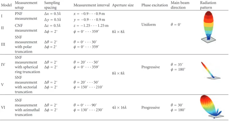
The frequency is 12 GHz, and the simulations are carried out in the three measurement setups under study. The mea-surement distance is 100λfor the three cases, and the sampl-ing spacsampl-ing and the size of the acquisition surfaces are indicated inTable 2in which the type of phase excitation and the aperture size are also presented. The objective is to gene-rate radiation patterns that steer in different directions with different beamwidths, especially to validate all of the trunca-tion cases that are considered in partial SNF measurements. As observed fromTable 2, Models I, II, and III are the same AUT but are measured in different scan surfaces. Models IV and V also have the same radiation pattern, but different acquisitions are employed in each of them. Finally, Model VI is measured using only one acquisition surface.

5. Critical Aspects of the Method

(8)

Table 2: Parameters of the simulated models.

Model Measurement setup

Sampling

spacing Measurement interval Aperture size Phase excitation

Main beam direction

Radiation pattern

I PNF measurement

Δx=0.5λ x= −0.9· · ·0.9 m

8λ×8λ

Uniform θ=0◦ Δy=0.5λ y= −0.9· · ·0.9 m

II CNF measurement

Δz=0.5λ z= −1.25· · ·1.25 m Δφ=2◦ φ=0◦· · ·359◦

III

SNF measurement with polar truncation

Δθ=2◦ Δφ=2◦

θ=0◦· · ·30◦ φ=0◦· · ·359◦

IV

SNF measurement with spherical ring truncation

Δθ=2◦ Δφ=2◦

θ=20◦· · ·50◦ φ=0◦· · ·359◦

8λ×8λ

Progressive θ=35 ◦

φ=180◦

V

Δθ=2◦ Δφ=2◦

θ=20◦· · ·50◦ φ=150◦· · ·210◦

VI

SNF measurement with azimuthal truncation

Δθ=2◦ Δφ=2◦

θ=0◦· · ·90◦

φ=130◦· · ·230◦ 4λ×16λ Progressive

θ=30◦ φ=180◦

detail. First, it is necessary to explain how to obtain the PWS on a regular grid in the spectral domain from near-field data that are obtained in the three measurement setups. Second, a modified definition of the spectral reliable region is presented. Finally, an eﬃcient algorithm to find the optimum termination point in the iterative method is proposed.

5.1. PWS on a Regularkx-kyGrid. As observed in the

des-cription of the method, the fast fourier transform algorithm is used to calculate the field distribution over the AUT plane from the PWS and vice versa. This algorithm is computa-tionally very eﬃcient, but it only works with samples that are distributed on a regular grid in both domains, that is, the samples of the extreme near-field are obtained on a regular

x-y grid, and the PWS must be known on a regularkx-ky

grid.

In the PNF case, the PWS is directly obtained in the required grid because it is calculated as an inverse fast fourier transform of the measured samples taken over a regularx-y

grid.

In CNF and SNF cases, additional steps are required because the classical near-field to far-field transformations produce the final results on a regular θ-φ grid. Diﬀerent calculation approaches can be used, but the easiest one is to employ an interpolation algorithm to obtain the samples on the desired grid. This solution introduces an interpolation error, but it does not require a great computational cost.

Two other approaches provide the exact values on the desired grid, but they are more complex. Both of them use the information that is contained in the spherical wave coeﬃcients (SWC), which are known in the SNF case, but

not in the CNF case. However, they can be easily obtained from the far-field pattern [3].

One of these two approaches employs the spherical-wave-expansion-to-plane-wave-expansion (SWE-to-PWE) transformation that is presented in [27] in which it is demon-strated that it is possible to define a rigorous transformation to derive the PWS from the SWC,

Pkx,ky,z

= ∞

n=1

n

m=−n

Q1(3)mnT1mn

kx,ky,z

+Q2(3)mnT2mn

kx,ky,z

,

(16)

whereQ(3)1mnandQ

(3)

2mnare the outgoing SWC, andT1mnand

T2mnare functions whose details can be found in [27].

The other approach evaluates the far-field pattern func-tions [3] on the desired directions that are defined by the regular kx-ky grid and calculates the far-field pattern as

follows:

EFF θ,φ

=L smn

Q(3)

smnKsmn θ,φ

, (17)

whereEFFis the far-field pattern,Lis a constant, andKare

the far-field pattern functions. Logically, when the far-field pattern is known, the PWS can be easily obtained by solving a system of two linear equations.

5.2. Spectral Reliable Region Employed in the Method. As

(9)

0 10 20 30 40 50 60 70 80 Iteration number

Using exact initial data

Using the calculated PWS withC=1 Using the calculated PWS withC=0.8 Using the calculated PWS withC=0.6 Using the calculated PWS withC=0.4

Er

ro

r

outside

the

reliable

re

gi

on

(%)

102

101

10−1

100

Figure 5: Error as a function of the iteration number using diﬀerent reliable regions.

0 10 20 30 40 50 60 70 80 Iteration number

Error outside the reliable region (%)

10 20 30 40 50 60 70 1

0.9 0.8 0.7 0.6 0.5 0.4 0.3

C

Figure 6: Error as a function of the iteration number and the parameterA.

but, after several iterations, it starts to increase. InSection 2, the classical definition of the spectral reliable region based on geometrical optics was presented. However, as noted in

Section 1, it is impossible to define a spectral region in which the error in the calculated far-field pattern is completely zero because of the unavoidable presence of ripple errors. There-fore, the error does not decrease monotonically in the iterative method. This eﬀect can be observed in Figure 5, where the error variation with the iteration number is repre-sented for the Model I using diﬀerent spectral reliable re-gions. The error in this figure is calculated as

εn(%)=

i /∈ΩREn θi,φi

−ER θi,φi2

i /∈ΩRER θi,φi

2 ·100, (18)

where En(θi,φi) and ER(θi,φi) are the electric field in the nth iteration and the reference electric field, respectively. As deduced from (18), only samples that are located outside of the reliable region are considered in the determination of the error.

Several conclusions can be extracted fromFigure 5. As expected, the error decreases monotonically when using the

Table 3: Redefinition of the maximum validity angles.

Measurement setup New maximum validity angles PNF measurement θx=C·θx;θy=C·θy CNF measurement θ

y=C·θy SNF measurement with

polar truncation θ

v=C·θv

SNF measurement with spherical ring truncation

θv1=θv1−(1−C)·(θv1−θv2)/2 θv2=θv2+ (1−C)·(θv1−θv2)/2

SNF measurement with azimuthal truncation

φv1=φv1+ (1−C)·(φv1−φv2)/2 φv2=φv2−(1−C)·(φv1−φv2)/2

θv1=θv1−(1−C)·(θv1−θv2)/2 θv2=θv2+ (1−C)·(θv1−θv2)/2 φv1=φv1+ (1−C)·(φv1−φv2)/2 φv2=φv2−(1−C)·(φv1−φv2)/2

Comparison between iterative results using diﬀerent initial data

5 10 15 20 25 30 35 40 45 50

5 10 15 20 25 30 35 40 Minimum

Number of iterations subset 1

N

umber

of

it

er

ations

subset

2

Figure 7: Gradient descent algorithm to find the optimum termination point.

exact initial data within the reliable region (see solid blue line). However, it is impossible to obtain those exact values because of the mentioned ripple errors. Then, in order to simulate the real behavior of the error, the PWS obtained from the truncated near-field acquisition is employed. Using this PWS and the spectral reliable region defined by geomet-rical optics and specified inTable 1, the error curve is as the red dashed line shows. In order to obtain a better conver-gence, the use of reliable regions smaller than that one defined by geometrical optics is considered. These new re-gions are determined by redefining the maximum validity angles, as indicated in Table 3 in which a weighting factor (C < 1) is introduced. The error variation for C = 0, 8,

(10)

Truncated field amplitude

v

u

0.5

0

−0.5

0.5 0

−0.5

0

−20

−40

−60

(a)

v

u

0.5

0

−0.5

0.5 0

−0.5

0

−20

−40

−60 Reconstructed field amplitude

(b)

v

u

0.5

0

−0.5

0.5 0

−0.5

0

−20

−40

−60 Truncated field error

(c)

v

u

0.5

0

−0.5

0.5 0

−0.5

0

−20

−40

−60 Reconstructed field error

(d)

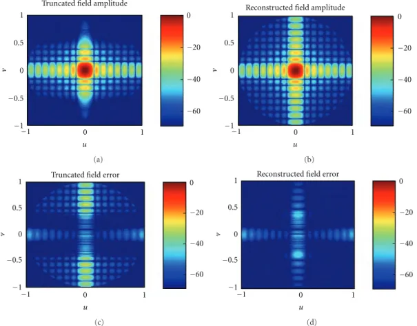
Figure 8: Far-field pattern and truncation error in dB before and after applying the iterative method for the Model I.

−80 −60 −40 −20 0 20 40 60 80 0

−5

−10

−15

−20

−25

−30

−35

−40

−45

−50

N

o

rmaliz

ed

amplitude

(dB)

θ(degrees) Reference pattern

Truncated pattern

Reconstructed pattern Validity

region

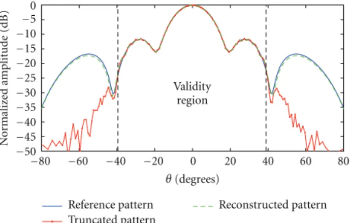
Figure 9: Comparison between the truncated, reconstructed and reference far-field patterns for the Model I in theφ=0◦cut.

of iterations and the parameterCis depicted for the Model I. As observed, very good results are obtained in the mentioned range ofC, with an error outside of the reliable region lower than 5%.

5.3. Algorithm to Determine the Proper Termination of the Iterations. Because of the impossibility of determining the

Figure 10: Measurement of a rectangular-horn antenna in a planar near-field range.

(11)

v

u

0.5

0

−0.5

0.5 0

−0.5

0

−20

−40

−60

−1

(a)

0

−20

−40

v

u

0.5

0

−0.5

0.5 0

−0.5

−1

(b)

0

−20

−40

v

u

0.5

0

−0.5

0.5 0

−0.5

−1

(c)

0

−20

−40

v

u

0.5

0

−0.5

0.5 0

−0.5

−1

(d)

Figure 11: Far-field pattern and truncation error in dB before and after applying the iterative method for the rectangular-horn measured in PNF.

N

o

rmaliz

ed

amplitude

(dB)

−80 −60 −40 −20 0 20 40 60 80

Truncated pattern

region 0

−5

−10

−15

−20

−25

−30

−35

−40

−45

−50

Figure 12: Comparison between the truncated, reconstructed and reference far-field patterns for the rectangular horn in theφ=90◦ cut.

in a diﬀerent way for the same value ofC. Therefore, when comparing the iterative results that were obtained in both cases, we will have a minimum when both results have the minimum error. This algorithm does not require additional measurements because two diﬀerent subsets of the measured near-field data can be used as inputs in the iterative method.

The iterative results obtained in both cases are stored and pairwise-compared to determine the optimum termination point for the two cases when the result of the comparison is minimum. The comparisons are carried out as follows:

μi j= Ei1 θ,φ

−Ej2 θ,φ

2

, (19)

whereEi1(θ,φ) and Ej2(θ,φ) are the reconstructed field in

theith iteration using the first data subset and the recon-structed field in thejth iteration using the second data sub-set, respectively.

(12)

v

u

0.5

0

−0.5

0

−20

−40

−60

−1 1

(a)

0

−20

−40

v

u

0.5

0

−0.5

−1 1

(b)

0

−20

−40

v

u

0.5

0

−0.5

−1 1

(c)

0

−20

−40

v

u

0.5

0

−0.5

−1 1

(d)

Figure 13: Far-field pattern and truncation error in dB before and after applying the iterative method for the Model II.

N

o

rmaliz

ed

amplitude

(dB)

Truncated pattern

region 0

−5

−10

−15

−20

−25

−30

−35

−40

−45

20 40 60 80 100 120 140 160

−50

Figure 14: Comparison between the truncated, reconstructed and reference far-field pattern for the Model II in theφ=90◦cut.

this algorithm, both the number of iterations and com-parisons may be drastically reduced, thereby requiring less computational time to obtain the minimum.

6. Numerical Results

To verify the accuracy of the proposed method, several exam-ples are analyzed. The objective is to validate the method in all of the cases that are described inFigure 1. This

valid-Figure 15: Measurement of a Ku-band reflector antenna in a cylindrical near-field range.

ation is carried out independently for each of these cases by employing both the simulated models defined inSection 4

and measured truncated near-field data.

6.1. Planar Near-Field Measurement. The method was

al-ready numerically validated for this type of measurement set-up in [17]. In this paper, another two examples are presented. The first example uses the information of simulated Model I where the maximum validity angles areθx = θy =17.75◦.

(13)

0

−20

−40

−60

v

u

0.5

0

−0.5

−1 1

(a)

0

−20

−40

v

u

0.5

0

−0.5

−1 1

(b)

0

−20

−40

v

u

0.5

0

−0.5

−1 1

(c)

0

−20

−40

v

u

0.5

0

−0.5

−1 1

(d)

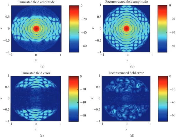
Figure 16: Far-field pattern and error in dB before and after applying the iterative method for the reflector measured in CNF.

N

o

rmaliz

ed

amplitude

(dB)

Truncated pattern

region

20 40 60 80 100 120 140 160 0

−10

−20

−30

−40

−50

−60

−70

Figure 17: Comparison among the truncated, reconstructed, and reference far-field patterns for the reflector in theφ=90◦cut.

of 1.5 m side. The results of the reconstruction are depicted in

Figure 8in which both the far-field and the truncation error before and after the application of the method are presented. As it is apparent, the proposed procedure provides a great reduction of the truncation error and retrieves the far-field pattern in the forward hemisphere with good accuracy. In this particular case, the error defined in (18) is reduced from 62.3% to 1.2%. The improvement achieved with the method is observed better inFigure 9, where a comparison among the

truncated, reconstructed and reference far-field patterns for theφ=0◦cut is shown.

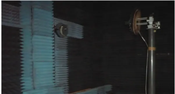
In the second validation, measured data were employed as input information to the proposed method. The measure-ment was carried out at 11 GHz using the PNF range in the anechoic chamber at the Technical University of Madrid (UPM). The probe and the AUT were selected to be a corru-gated conical-horn antenna and a rectangular-horn antenna, respectively, and they were separated from each other by 1.3 m (seeFigure 10). When both antennas were mounted on their respective positioners, a measurement over a 2.7 m×

2.7 m acquisition plane was recorded. The same AUT was previously measured in a SNF range in order to obtain a reference pattern for comparison with the results obtained with the presented method.Figure 11shows a comparison between the truncated and reconstructed far-field patterns and the error before and after applying the method. As in the previous example, a great improvement of the accuracy outside of the reliable region is achieved, which reduces the error from 79.3% to 7.1%. Another comparison is presented inFigure 12.

6.2. Cylindrical Near-Field Measurement. As commented

(14)

0

−20

−40

−60

0

−20

−40

−60

0

−20

−40

−60

0

−20

−40

Truncated field error Reconstructed field error

v

u

0.5

0

−0.5

−1 1

v

u

0

−1 1

v

u

0

−1 1

v

u

0

−1 1

(a)

0

−20

−40

−60

0

−20

−40

−60

0

−20

−40

−60

0

−20

−40

v

u

0

−1 1

v

u

0

−1 1

v

u

0

−1 1

v

u

0

−1 1

(b)

(15)

v

u

0

−20

−40

−60

0

−20

−40

−60

0

−20

−40

−60 0

−20

−40

−1 1

v

u

0

−1 1

v

u

0

−1 1

v

u

0

−1 1

(c)

0

−20

−40

−60

0

−20

−40

−60

0

−20

−40

−60 0

−20

−40

v

u

0

−1 1

v

u

0

−1 1

v

u

0

−1 1

v

u

0

−1 1

(d)

(16)

N

o

rmaliz

ed

amplitude

(dB)

θ(degrees) Validity

region 0

−10

−20

−30

−40

−50

−60

−70

−80 −60 −40 −20 0 20 40 60 80

(a)

N

o

rmaliz

ed

amplitude

(dB)

θ(degrees) Validity

region 0

−10

−20

−30

−40

−50

−60

−70

−80 −60 −40 −20 0 20 40 60 80

(b)

N

o

rmaliz

ed

amplitude

(dB)

Truncated pattern

region 0

−10

−20

−30

−40

−50

−60

−70

−80 −60 −40 −20 0 20 40 60 80

(c)

N

o

rmaliz

ed

amplitude

(dB)

Truncated pattern

region 0

−10

−20

−30

−40

−50

−60

−70

−80 −60 −40 −20 0 20 40 60 80

(d)

Figure 19: Comparison between the truncated, reconstructed and reference far-field patterns for the Models III (a), IV (b), V (c), and VI (d) in theφ=0◦_cut.

Figure 20: Measurement of an X-band array antenna in spherical near-field.

in this second part of the numerical results, cylindrical near-field data are employed as input to the iterative method in order to demonstrate its eﬀectiveness in this type of meas-urement setup.

Logically, because the method uses information about the PWS, only the truncation error in the forward hemi-sphere may be suppressed. The validation is carried out, as in the previous case, by employing both simulated and meas-ured data. First, the simulated Model II that is described in Table 2 is used. According to the geometrical optics, in this first example, only the far-field pattern in the spectral region defined by|v|<sin(24.7◦) can be considered reliable. However, after the application of the method, it is possible

to retrieve the pattern in the whole forward hemisphere with good accuracy, as observed in Figure 13. As in the previous examples, one far-field cut comparison is depicted inFigure 14.

The method was also validated with measured near-field data. The measurement was performed in the CNF range at the UPM. For the experiment, the probe and the AUT consisted of a corrugated conical-horn antenna and a Ku-band reflector with a 40 cm diameter (seeFigure 15), respectively. The data were acquired over a cylinder with a height of 2.7 m and a radius of 2.3 m and with a spatial sampling equal to 0.5λin the vertical direction and 2.5◦ in the azimuth. As in the PNF case, the AUT was also measured in a whole sphere in order to obtain a reference pattern. From inspection ofFigure 16, it is evident that the truncation error is greatly suppressed, reducing the error expressed in (18) from 58.2% to 8.9%. A comparison depicted inFigure 17

shows the reconstructed far-field pattern in the vertical plane versus the truncated and reference far-field pattern.

6.3. Spherical Near-Field Measurement. Finally, the capability

(17)

0

−20

−40

−60

v

u

0

−1 1

(a)

0

−20

−40

v

u

0

−1 1

(b)

0

−20

−40

v

u

0

−1 1

(c)

0

−20

−40

v

u

0

−1 1

(d)

Figure 21: Far-field pattern and error in dB before and after applying the iterative method for the array antenna measured in SNF with polar truncation.

N

o

rmaliz

ed

amplitude

(dB)

Truncated pattern

region 0

−10

−20

−30

−40

−50

−60

−70

−80 −60 −40 −20 0 20 40 60 80

Figure 22: Comparison between the truncated, reconstructed and reference far-field pattern for the array in theφ=0◦cut.

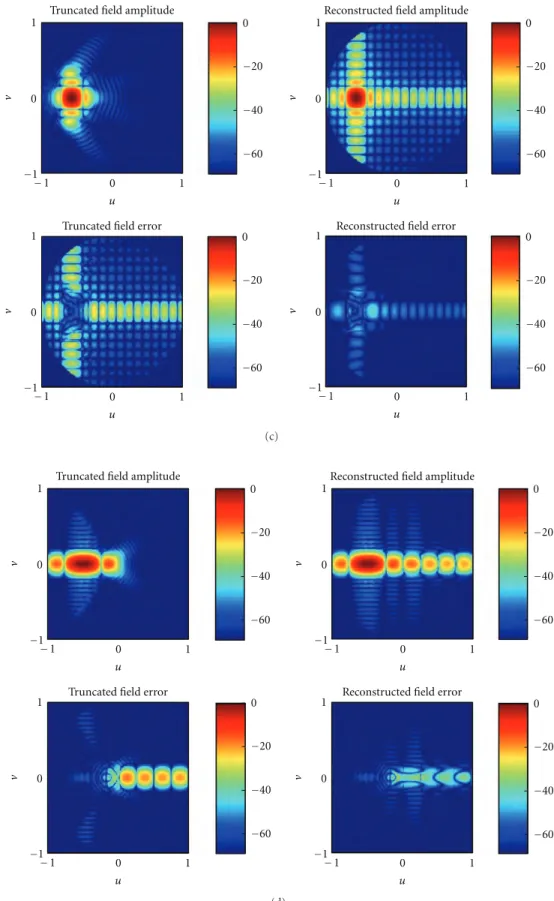
regions. In this work, four types of truncation in the SNF measurements are considered (see Figure 2). The last four simulated models presented inSection 4are used to analyze the eﬀectiveness of the method in each of these truncations. All of the results are shown in Figures18and19, and they contain the far-field pattern and the error before and aft-er applying the method, as well as a comparison among

the reconstructed, truncated, and reference patterns in one plane, as in the previous examples.

The proposed iterative method was also applied to meas-ured spherical near-field data. The acquisition was per-formed in the SNF range at the UPM. The AUT was per-formed by a square array of 256 printed elements covering a large bandwidth in the X-band, and its dimensions were 40 cm× 40 cm. The array was divided into 16 square subarrays of 4 elements ×4 elements (see Figure 20). Data were taken in a whole sphere with a spatial sampling equal to 2◦ both in azimuth and elevation. Because the AUT is steering at broadside, the most appropriate truncation is a polar truncation. Therefore, only measured data from θ = 0◦ to θ = 20◦ were used as input for the method. After the application of the iterative procedure and comparison with the reference pattern from the whole measurement, the results in Figures 21 and 22 were obtained, in which the truncation error is greatly reduced, as in the previous exam-ples. In this last case, the error of (18), which has been con-sidered to be the quality factor, is reduced from 82.5% to 8.6%.

7. Conclusions

(18)

near-field setup has been proposed in this paper. The method is based on the Gerchberg-Papoulis iterative algo-rithm used to extrapolate band-limited functions, and it is a generalization of the approach presented in [17] for the planar case. Therefore, the proposed method can be viewed as a continuation of the work developed in [17], not only extending its applicability, but also introducing new algorithms to reduce the computational time required to remove the truncation errors. The convergence of this meth-od has been mathematically demonstrated. Moreover, a de-tailed study of the spectral reliable region for each type of measurement setup and an analysis of critical aspects of the method has been performed. Finally, the method has been validated by using both simulated and measured near-field data, showing that it is possible to reduce the truncation errors eﬀectively. It was noted that the proposed method works well for planar aperture antennas because the antenna aperture, in which the fields are assumed to be concentrated, is well defined.

Acknowledgments

This work was developed with the support of the Spanish FPU Grant for Ph.D. students and the financing of the Crocante Project (TEC2008-06736-C03-01/TEC). F. J. Cano-F´acila would also like to thank DTU Electrical Engineering for its support during his stay at the Technical University of Denmark.

References

[1] A. D. Yaghjian, “An overview of near-field antenna measure-ments,” IEEE Transactions on Antennas and Propagation, vol. AP-34, no. 1, pp. 30–44, 1986.

[2] H. G. Booker and P. C. Clemmow, “The concept of an angular spectrum of plane waves, and its relation to that of polar diagram and aperture distribution,” Proceedings of the IEEE:

Radio and Communication Engineering, vol. 97, no. 45, pp. 11–

17, 1950.

[3] J. E. Hansen, Ed., Spherical Near-field Antenna Measurements, Peter Peregrinus, London, UK, 1988.

[4] W. M. Leach and D. T. Paris, “Probe compensated near-field measurements on a cylinder,” IEEE Transactions on Antennas

and Propagation, vol. AP-21, no. 4, pp. 435–445, 1973.

[5] P. R. Rousseau, “The planar near-field measurement of a broad beam antenna using a synthetic subarray approach,” in

Pro-ceedings of the IEEE Antennas and Propagation Society Interna-tional Symposium Digest, pp. 160–163, Montreal, Canada, July

1997.

[6] T. Al-Mahdawi, “Planar near-field measurement of low direc-tivity embedded antennas using a synthetic array probe tech-nique,” in Proceedings of the IEEE International Antennas and

Propagation Symposium Digest, pp. 1311–1314, June 1998.

[7] E. B. Joy, “Windows ’96 for planar near-field measurements,” in Proceedings of the Antenna Measurement Techniques

Associ-ation, pp. 80–85, 1996.

[8] E. B. Joy, C. A. Rose, A. H. Tonning, and EE6254 Students, “Test-zone field quality in planar near-field measurements,” in

Proceedings of the Antenna Measurement Techniques Associa-tion, pp. 206–210, Williamsburg, Va, USA, November 1997.

[9] P. Petre and T. K. Sarkar, “Planar near-field to far-field trans-formation using an equivalent magnetic current approach,”

IEEE Transactions on Antennas and Propagation, vol. 40, no.

11, pp. 1348–1356, 1992.

[10] S. F. Gregson, C. G. Parini, and J. McCormick, “Development of wide-angle antenna pattern measurements using a probe-corrected polyplanar near-field measurement technique,” vol. 152, no. 6, pp. 563–572.

[11] O. M. Bucci, G. D’Elia, and M. D. Migliore, “New strategy to reduce the truncation error in near-field/far-field transforma-tions,” Radio Science, vol. 35, no. 1, pp. 3–17, 2000.

[12] O. M. Bucci, C. Gennarelli, and C. Savarese, “Representation of electromagnetic fields over arbitrary surfaces by a finite and nonredundant number of samples,” IEEE Transactions on

An-tennas and Propagation, vol. 46, no. 3, pp. 351–359, 1998.

[13] J. C. Bolomey, O. M. Bucci, L. Casavola, G. D’Elia, M. D. Mig-liore, and A. Ziyyat, “Reduction of truncation error in near-field measurements of antennas of base-station mobile com-munication systems,” IEEE Transactions on Antennas and

Pro-pagation, vol. 52, no. 2, pp. 593–602, 2004.

[14] F. D’Agostino, F. Ferrara, C. Gennarelli, R. Guerriero, and G. Riccio, “An eﬀective technique for reducing the truncation error in the near-field-far-field transformation with plane-polar scanning,” Progress in Electromagnetics Research, vol. 73, pp. 213–238, 2007.

[15] O. M. Bucci and M. D. Migliore, “A new method for avoiding the truncation error in near-field antennas measurements,”

IEEE Transactions on Antennas and Propagation, vol. 54, no.

10, pp. 2940–2952, 2006.

[16] L. Infante, E. Martini, A. Peluso, and S. Maci, “The shadow boundary integral for the reduction of the truncation error in near-field to far-field transformations,” in Proceedings

of the IEEE Antennas and Propagation Society International Symposium, pp. 416–419, Washington, DC, USA, July 2005.

[17] E. Martini, O. Breinbjerg, and S. Maci, “Reduction of trunca-tion errors in planar near-field aperture antenna neasurements using the Gerchberg-Papoulis algorithm,” IEEE Transactions

on Antennas and Propagation, vol. 56, no. 11, pp. 3485–3493,

2008.

[18] R. W. Gerchberg, “Super-resolution through error energy re-duction,” Optica Acta, vol. 21, no. 9, pp. 709–720, 1974. [19] A. Papoulis, “A new algorithm in spectral analysis and

band-limited extrapolation,” IEEE Transactions on Circuits and

Sys-tems, vol. 22, no. 9, pp. 735–742, 1975.

[20] M. Serhir, J. M. Geﬀrin, A. Litman, and P. Besnier, “Aperture antenna modeling by a finite number of elemental dipoles from spherical field measurements,” IEEE Transactions on

An-tennas and Propagation, vol. 58, no. 4, Article ID 5398845, pp.

1260–1268, 2010.

[21] K. T. Kim, “Truncation-error reduction in 2D cylindri-cal/spherical near-field scanning,” IEEE Transactions on

Anten-nas and Propagation, vol. 58, no. 6, pp. 2153–2158, 2010.

[22] K. T. Kim, “Truncation-error reduction in acoustic spherical near-field scanning,” in Proceedings of the Antennas and

Propa-gation Society International Symposium, (APSURSI ’10),

Tor-onto, Canada, July 2010.

[23] A. Papoulis, Signal Analysis, McGraw-Hill, New York, NY, USA, 1977.

[24] R. C. Wittmann, C. F. Stubenrauch, and M. H. Francis, “Sp-herical scanning measurements using truncated data sets,” in

(19)

[25] E. Martini, S. Maci, and L. J. Foged, “Spherical near field measurements with truncated scan area,” in Proceedings of the

European Conference on Antennas and Propagation, pp. 3412–

3414, Rome, Italy, April 2004.

[26] A. D. Yaghjian, “Upper bound errors in far-field antenna para-meters determined from planar near-field measurements,” NBS Technical Report 667, National Bureau of Standards, Boulder, Colo, USA, 1975.

[27] C. Cappellin, Antenna diagnostic for spherical near-field

anten-na measurements, Ph.D. thesis, Departament of Electrical