1 2 3 4 5 6 7 8 9 10 11 12 13 14 15 16 17 18 19 20 21 22 23 24 25 26 27 28 29 30 31 32 33 34 35 36 37 38 39 40 41 42 43 44 45 46 47 48 49 50 51 52 53 54 55 56 57 58 59 60 61 62 63 64 65
-1-
Pore size analysis from retention of neutral solutes through nanofiltration
membranes. The contribution of Concentration-Polarization.
Noemi GARCÍA-MARTÍNa, Verónica SILVAa, F.J. CARMONAb, Laura PALACIOa*, Antonio HERNÁNDEZa and Pedro PRÁDANOSa
a
. Grupo de Superficies y Materiales Porosos (SMAP, UA-UVA-CSIC), Dpto. de Física Aplicada, Facultad Ciencias, Universidad de Valladolid, 47071 Valladolid, Spain
b
. Dpto. de Física Aplicada. Escuela Politécnica, Universidad de Extremadura, 10004, Cáceres, Spain
* Corresponding author.
Laura PALACIO. Phone number: +34 983 423943 Email address: [email protected]
ABSTRACT
Pore size distribution is one of the most important characteristics of a membrane. This can be obtained from the fitting of pore radius calculated from retention versus flux measurements for a set of solute solutions. In this work a set of non-charged similar molecules are chosen as solutes to minimize other interactions apart of those related to size. The hydrodynamic model will be used to characterize the behavior of the membrane to uncharged solutes, assuming that membrane pores are straight and cylindrical.
As is known, the phenomenon of concentration polarization must be taken into account because true retention is not experimentally accessible by concentration measurements. Frequently, the film layer model is applied for the dependence of concentration with experimental conditions; but the application of this model requires prior knowledge of the mass transfer coefficient which is evaluated by different dimensionless correlations (Sherwood correlation). Here we show a review of different alternatives in doing it and analyze their consequences when computing the pore size distribution.
Experimental data were obtained from dead-end filtration experiments of a set of four ethylene glycols solutions with a nanofiltration membrane. Obtained results show the importance of the mass transfer model in the pore size value obtained.
Keywords: Nanofiltration; Mass transfer; Retention; Pore size distribution *Manuscript
1 2 3 4 5 6 7 8 9 10 11 12 13 14 15 16 17 18 19 20 21 22 23 24 25 26 27 28 29 30 31 32 33 34 35 36 37 38 39 40 41 42 43 44 45 46 47 48 49 50 51 52 53 54 55 56 57 58 59 60 61 62 63 64 65
-2- 1. Introduction
Membranes have found a broad range of application in an endless list of production sectors, such as food, gases, pharmaceuticals, or water. The pressure driven membrane processes are frequently classified in four big groups: microfiltration (MF), ultrafiltration (UF), nanofiltration (NF) and reverse osmosis (RO) membranes. The last two are the most important ones when the issue is desalination or purification of water [1]. Taking into account the economic importance of the two most common purposes of such processes, watering and human consumption, one can imagine the amount of resources devoted to improving the characterization and optimization of membranes made for these objectives. This membrane characterization can be focused on the structural or functional aspects. Between those belonging to structural characterization, the pore size distribution plays an important role in determining the membrane retention, especially in the case of uncharged solutes.
1 2 3 4 5 6 7 8 9 10 11 12 13 14 15 16 17 18 19 20 21 22 23 24 25 26 27 28 29 30 31 32 33 34 35 36 37 38 39 40 41 42 43 44 45 46 47 48 49 50 51 52 53 54 55 56 57 58 59 60 61 62 63 64 65
-3-
resonance imaging, radio isotope labeling, electron diode array microscope or direct pressure measurements as is reviewed in [12]. Moreover, unfortunately, these techniques are at present far from being unambiguous.
To solve this problem, the film layer model is usually applied to describe the dependence of concentration with experimental conditions [13]. In this model, the mass transfer coefficient is related with the Schmidt, Reynolds and Sherwood numbers (named Sc, Re and Sh respectively) through the so called Sherwood correlation [14]. In this work the coefficients of this correlation are reviewed because different values have been used for the same fixed parameter without any clear criteria to do so.
Once the true retentions for each solute have been determined, the pore radius is calculated as the fitting parameter of the “Steric pore flow model” (SPFM) [2, 15] from data for each solute filtration; the knowledge of both the solute and pore sizes allows building the pore size distribution.
In this work, experimental data are obtained from a set of four filtrations of a small lineal ethylene glycols solution by a typical NF membrane. This set of non-charged solutes was chosen to minimize the differences in the interactions pore-solute apart from volume (or size).
The hydrodynamic model will be used to characterize the behavior of the membrane to uncharged solutes; assuming that the membrane pores are straight cylinders where diffusion and concentration gradients are the forces acting for the solute transport.
2. Theory
1 2 3 4 5 6 7 8 9 10 11 12 13 14 15 16 17 18 19 20 21 22 23 24 25 26 27 28 29 30 31 32 33 34 35 36 37 38 39 40 41 42 43 44 45 46 47 48 49 50 51 52 53 54 55 56 57 58 59 60 61 62 63 64 65
-4-
The separation selectivity of a nanofiltration membrane is governed by three processes: transport along the pores, partitioning through the membrane-solution interfaces and transport through the polarization layer [17].
The first two of these phenomena depend essentially on the behavior of the chemical potential. The first one is governed by the first Ficks’s law or by the extended Nernst-Planck equation if convection is included. The second one is based on the equality of chemical potentials at both sides of each interface. Meanwhile, the third phenomenon is governed by the hydrodynamics of the filtration set, essentially given by the mass transfer coefficient, which depends on the set-up configuration and experimental conditions.
2.1. Chemical potential
Chemical potential of a species s under isothermal conditions is given by [17]:
00
0 s
s s ( , ) s
0
' d ' ln
p
T p p
a
V p p kT W
a
(1)where 0
0 s ( ,T p )
is the standard chemical potential,p0 the reference pressure, and V the partial molar volume in the standard state. as is the solute activity, being a0 the activity for the standard state. And Ws quantifies the interaction free energy including all interactions of the solute with the medium not included into activity; for neutral molecules, only the purely steric interaction must be considered.
2.2. Membrane Partition Coefficient
Each side of the membrane defines an interface. Assuming there is equilibrium between both phases (bulk phase, and membrane phase), both chemical potentials must be equal:
s,b s,m
(2)
1 2 3 4 5 6 7 8 9 10 11 12 13 14 15 16 17 18 19 20 21 22 23 24 25 26 27 28 29 30 31 32 33 34 35 36 37 38 39 40 41 42 43 44 45 46 47 48 49 50 51 52 53 54 55 56 57 58 59 60 61 62 63 64 65
-5-
only purely steric effects determine this ratio, which coincides with the steric partitioning coefficient. Assuming that flow through a membrane takes place along the
x-axis direction, being x=0 and x=∆x the coordinates for the interfaces, and denoting by - and + the left and right sides of each interface, the membrane partition coefficient [19, 20] is:
s,m s s
s
s,b s s
(0 ) ( )
(0 ) ( )
c c c x
K
c c c x
(3)
Different expressions for , the steric partitioning factor, can be obtained depending on the geometry of the pore, cylindrical, slit, etc. In terms of , the ratio between solute and porous radius,rs /rp,for cylindrical pores (1)2 [20-22].
2.3. Transport Equation
The membrane pores, supposed oriented along the x-direction, have a length ∆x, and a radius rp . The transport of a species through them is described by the Nernst-Planck Equation:
s,p s s
s s s
D c d
j c v
RT dx
(4)
The flux of species s, js, is given by the sum of a diffusion term and a convective one. In the diffusion term, cs is the solute concentration, Ds,p is the diffusivity inside the pore and μ is the chemical potential. The hindering effect introduced by pore walls on solute transport is taken into account by means of the hindrance factors. The hindrance factor for diffusion, Kd, relates the diffusion coefficients inside (Ds,p) and outside (Ds,b) the poreDs,p K Dd s,b. The hindrance factor
for convection relates the solute (vs) and the solvent (vw) speeds into the pore: vs K vc w
.
By assuming that:
- Inside the pore there is no change in the interactions of the solute with the medium
- An activity coefficient equal to unity
1 2 3 4 5 6 7 8 9 10 11 12 13 14 15 16 17 18 19 20 21 22 23 24 25 26 27 28 29 30 31 32 33 34 35 36 37 38 39 40 41 42 43 44 45 46 47 48 49 50 51 52 53 54 55 56 57 58 59 60 61 62 63 64 65 -6-
the gradient of the chemical potential needed in Eq. (4) reduces, to:
d dp RT dc V
dx dx c dx
(5)
Here Vhas been assumed to be almost independent of pressure. After introducing hindrance factors and Eq. (5) for the gradient of the chemical potential into equation for transport, Eq. (4), we obtain:
s
s d s,b c s w
c dp dc
j K D V K c v
RT dx dx
(6)
Different correlations have been proposed in the literature for the hindrance factors [19, 22, 23]. Dechadilok and Deen [21], in addition to analyzing some of these proposals, study and present a way of introducing the effect of pressure gradient in theses hindrance factors. Expressions for Kc and Kd used in this work are those proposed in the cited work by Dechadilok and Deen in 2006 [21]. For cylindrical pores:
2 3 4
5 6 7
2 3
2
d 2
c
9
1 ln 1.5603 0.52815 1.9152 2.8190
8
0.27078 1.10115 0.43593
1 3.867 1.907 0.834
1 1.867 0.741
1 1 K K (7)
The correction due to pressure effects were studied in recent analysis [24] and leads to changing Kc and Kd by K’c and K’d for cylindrical pores as follows:
2 '
c c d
' d d
16 2 9
K K K
K K
(8)
In terms of , the ratio between solute and porous radius, note that the steric partitioning factor (1)2. Then taking into account that:
s s
w
k
V V k k
J j A
J j A v A
(9)
correlate the fluxes per unit of pore area to those per unit of membrane area through the membrane porosity Ak, we arrive to
s s
d s,b k 'c s V
J dc
K D A K c J
dx
1 2 3 4 5 6 7 8 9 10 11 12 13 14 15 16 17 18 19 20 21 22 23 24 25 26 27 28 29 30 31 32 33 34 35 36 37 38 39 40 41 42 43 44 45 46 47 48 49 50 51 52 53 54 55 56 57 58 59 60 61 62 63 64 65 -7-
The presence in Eq. (10) of K’c and K’d makes impossible a direct comparison with Eq. (6) because pressure effects are included now in these modified constants [25]. It is worth noting that, in essence, the effect of pressure taken into account in Eqs. (8) and (10) correspond to the coupling between convection and diffusion.
2.4. Concentration Polarization
When a membrane is used with a solution containing dissolved or suspended species, the phenomenon of concentration-polarization must be taken into account [26-30]. The presence of polarization layer involves the retention coefficient definition:
- Observed retention: Feed and permeate concentration measurement, cs,f and cs,p respectively, allow the evaluation of the observed retention as
s,p o s,f 1 c R c
(11)
when the permeate concentration arrives to be constant.
- True retention, defined in terms of cs,p and cs,m, the solute concentration in the permeate and on the membrane-feed side.
s,p
s,m 1 c
R c
(12)
Since true retention is not experimentally accessible by concentration measurements, other alternatives must be sought.
From Eq. (10), the Peclet number (Pe’) – that corresponds to the ratio of the
convective to diffusive contributions– can be defined as:
'
' c
d s,b v
k
K J x
Pe
K D A
(13)
The retention of the actual membrane, or true retention coefficient, can be expressed as a function of the pore radius, through [24, 31]:
' s,p c ' ' s,m c 1- =11 1 Pe
c K
R
c K e
1 2 3 4 5 6 7 8 9 10 11 12 13 14 15 16 17 18 19 20 21 22 23 24 25 26 27 28 29 30 31 32 33 34 35 36 37 38 39 40 41 42 43 44 45 46 47 48 49 50 51 52 53 54 55 56 57 58 59 60 61 62 63 64 65
-8-
Note that this retention coefficient depends now not only of the membrane but also on the rest of the experimental device (cell design, stirrer, etc.) which determines the flux condition on the membrane and control the solute accumulation on the membrane-feed side (making cs,m cs,f). The true retention coefficient, R, is higher than
Ro due to the effect of concentration polarization.
To solve the problem of determining true retention coefficients, a model is usually applied for the dependence of the concentration on the membrane with experiment conditions [13]. The film layer model for concentration polarization predicts that:
/ s,m s,p ( s,f s,p)
v m
J K
c c c c e (15)
where Km is the mass transfer coefficient. Any viscosity increase or change in
diffusivity is usually assumed although it could appear due to the increase of concentration when approaching the membrane surface. Suction effect has been considered sometimes [32].
When expression (15) for cm is introduced into Eq. (12), the true retention coefficient is related with the observed one by:
o o
1 1
ln ln v
m
R R J
R R K
(16)
The mass transfer coefficient can be related with the Schmidt, Reynolds and Sherwood numbers (named Sc, Re and Sc respectively) through the so called Sherwood correlation [14]:
Sh A Re Sc (17)
In this equation, A, and are parameters that depend on the configuration of the experimental setup (tangential flow or cross flow, laminar or turbulent, etc.). For the specific case of a stirred cell, the three dimensionless numbers are defined as:
2
c, c ,
m
K r r
Sh Re Sc
D D
1 2 3 4 5 6 7 8 9 10 11 12 13 14 15 16 17 18 19 20 21 22 23 24 25 26 27 28 29 30 31 32 33 34 35 36 37 38 39 40 41 42 43 44 45 46 47 48 49 50 51 52 53 54 55 56 57 58 59 60 61 62 63 64 65
-9- c
r is the radius of the cell or stirrer length, is the stirring speed, D is the diffusivity of the solute and and are the viscosity and the density respectively. Actually rc should be a geometrical parameter characteristic of the dispositive and process.
The substitution of Eq. (18) into Eq. (17) gives us a dependence of the mass transfer coefficient with the cell geometry, solvent physical properties, nature of the solute and stirring speed:
2 1 1 1 1
c ' '' '''
m
K Ar D A D A D A (19)
The parameter A’ depends on the geometry of the cell. A’’ depends on the liquid
because includes the viscosity and density values. If low concentrations are used in the experiments, these magnitudes can be assumed as those for the pure solvent (water). A’’’
depends also on the solute through the solute infinite dilution coefficient.
For each filtrated solution, the mass transfer coefficient should be proportional to. Substitution of Eq. (19) into Eq. (16) produces a relationship between the observed retention and the ratio Jv/
.
o o
1 1 1
ln ln
''' v
R R J
R R A
(20)
When Jv increases, cs,m also does (and consequently R) until a stable value is achieved. When this maximum retention, Rmax, is obtained -for high Jv values-
expression of Eq. (20) corresponds to a straight line as the first summand of the
right-hand side would be also constant, ln 1
Rmax
Rmax. This procedure to find themaximal retention and the mass transfer coefficient Km A'''
is called the velocity
variation method [33-35].
The fit of a set of experimental data of ln 1
R0
R0 versus Jv/
to Eq.
(20) will provide A’’’ as the inverse of the slope. In addition, Rmax, can be obtained from the intercept. Once Km is known, the true retention coefficient can be calculated by Eqs.
(15) and (16).
1 2 3 4 5 6 7 8 9 10 11 12 13 14 15 16 17 18 19 20 21 22 23 24 25 26 27 28 29 30 31 32 33 34 35 36 37 38 39 40 41 42 43 44 45 46 47 48 49 50 51 52 53 54 55 56 57 58 59 60 61 62 63 64 65
-10-
flux is predominant, leading to an approximately constant cs,p cs,m and R approaching a
constant Rmax.
2.5. Pore size distribution by solute retention
The fit of real retention R versus Jv, according to the model presented in sections
2.1 to 2.3 provides an estimation of the pore radius, rp, which is different for each solute, with radius rs. This permits an evaluation of the pore size distribution [3, 36-38] herein we summarize the fundamentals of the methodology founded by Tkacik and Michaels [39].
In order to evaluate the pore size distribution of a partially retaining membrane when retention is due to a pure sieving mechanism, we assume that for each solute there is a fraction of totally retaining pores while the rest of them allow a free pass of the molecules. Then we can write the mass balance for each solute as
s,p ,t s,m
V V
J c J c (21)
Where Jv is the total volumetric flux and Jv,t is the volumetric flux transmitted through the non-rejecting (transmitting) fraction of pores. On the other hand, the ratio of the transmitted volumetric flux, Jv,t, and pure water flux, Jw,t, passing through the transmitting pores is:
,t m
w ,t 0
V
J
J
(22)
ηm and η0 are the solution and solvent viscosities respectively. But for low cs,m this ratio can be approximated by 1 in such a way that Eq. (22) can be rewritten as,
W, t V(1 ) W, r V
J J R J J R (23)
Note that Eq. (23) is applicable when dealing with low concentrations and not too strong concentration polarization. According to Eq. (23), Jw,t and Jw,r (pure water flux passing through the retentive pores, Jw Jw, tJw, r) can be evaluated once JV for
1 2 3 4 5 6 7 8 9 10 11 12 13 14 15 16 17 18 19 20 21 22 23 24 25 26 27 28 29 30 31 32 33 34 35 36 37 38 39 40 41 42 43 44 45 46 47 48 49 50 51 52 53 54 55 56 57 58 59 60 61 62 63 64 65
-11-
the solute. Thus if many solutes with different sizes are used the cumulative pore size distribution could be obtained [36].
To reproduce the experimental data, different sigmoid curves with horizontal asymptotes at Jw,t /Jw 1 and Jw,t /Jw 0 have been used
,
p;
w t
i w
J
F r a
J (24)
where {ai} is a set of constants to be evaluated by fitting Eq. (24) to experimental
results. In this case only two-parameter distributions will be used (being a1 and a2 these parameters):
The derivative, f r( )=dp F r( ) / d =d(p rp Jw,t/Jw) / drp, is the probability density
function (PDF) and provides the flux distribution through differently sized pores. As the flow is proportional to the fourth power of the pore radius, 4
p
r (according to the Hagen Poiseuille equation); the pore size distribution, except by a normalization constant, could be obtained as:
w w,t
t
p 1 2
4 4
p p p p
d( / )
d( / ) 1 1
( ; , )
d d
J J N N
f r a a
r r r r (25)
2.6. Diffusion coefficients estimation
Within the model proposed here, diffusivities for each of the solutes in solution must be known to be used in Eqs. (10) and (18). The diffusion coefficients are also needed to evaluate the radii of the solutes in terms of the Stokes-Einstein equation:
6
kT D
r
(26)
1 2 3 4 5 6 7 8 9 10 11 12 13 14 15 16 17 18 19 20 21 22 23 24 25 26 27 28 29 30 31 32 33 34 35 36 37 38 39 40 41 42 43 44 45 46 47 48 49 50 51 52 53 54 55 56 57 58 59 60 61 62 63 64 65
-12-
12 1 2 3
ln(D )A A /TA c (27)
c=0 was taken and T=298.15 K to extrapolate experimental data to the working temperature, the obtained values of infinite dilution diffusion coefficients of glycols in water are show in Table 1. These values show good agreement with some others found in literature [42-44]. Table 1 also presents the Stokes radii corresponding to each solute according to Eq. (26).
2.7. Reynolds number
The Reynolds number corresponds to the ratio between inertial forces to viscous forces. In the particular case of this work, the definition of the Reynolds number for a stirred cell is given by Eq. (18).
The two sources of debate within the different authors are the choice of an appropriate typical length and velocity. Therefore, different chemical engineering handbooks of common use give different definitions for Re. About the choice for the typical length, this can be chosen as the length of the stirring bar (dsb),
2 C&R sb/
Re fd , as in [45] or as the cell or tank diameter (RePerry's dcell2 /) as is
showed in the Perry’s chemical Engineerings’ Handbook [46]. Some other authors also use the tank size, but in terms of the radius ( 2
tank tank/
Re r ) [47, 48]. This criterion
is also indicated by Schäfer et al [49]. Because, in this work, dead-end experiments were done using a un-baffled stirred cell, this characteristic length should be the cell radius as suggested by Schäfer et al. [49] and written in Eq. (18), which is the most usual convention.
There are also some discrepancies in the units of the stirrer speed. Some authors choose the frequency, f, in s-1 or the angular speed, ω, in rad·s-1. If the stirrer length is written as a fraction of cell diameter, rsb rcell with 1, both discrepancies are only
a linear scaling of the Reynolds number. In this way: 2
C&R (2 / ) tank
Re Re (
C&R 0.637 tank
Re Re ) [45] and RePerry's 4Retank [46].
1 2 3 4 5 6 7 8 9 10 11 12 13 14 15 16 17 18 19 20 21 22 23 24 25 26 27 28 29 30 31 32 33 34 35 36 37 38 39 40 41 42 43 44 45 46 47 48 49 50 51 52 53 54 55 56 57 58 59 60 61 62 63 64 65
-13-
The choice for Sherwood relation parameters of Eq. (17) depends largely on the flow regime defined by the value of the Reynolds number; for that reason it is very convenient to analyze the laminar and turbulent intervals once the definition of Re has been discussed.
2.8. Sherwood relation
Colton and Smith [50] made a theoretical review and fitting of experimental data to the different studied models. In that work, Colton and Smith compared these results with previously proposed correlations: Kaufmann and Leonard suggested [51] =0.68 and =1/3; Calberbank and Moo-Young [52]for agitation under turbulent conditions (Re>40000) used =0.7 and =1/3; Marangozis and Johnson [53] recommended =0.70 and =1/3 (also for Re>40000). The theoretical study for a turbulent boundary layer using the Chilton-Colburn analogy[54], following the approach of Eckert and Jackson (1951)[55], gives =0.8 and =1/3. The fit of experimental data for mass transfer coefficients establishes that for 8000 < Re < 32000 =0.567 while =0.746 for 32000 <
Re < 82000. Coulson et al. indicated that the transition between laminar and turbulent regimes is determined by ReC&R values between 1000 and 2000, which corresponds with
Re between 8441 and 16882 [45].
Some frequently cited Chemical Engineering handbooks refer to different works in this question. Rousseau [56] citing Kaufmann and Leonard assign =0.68 and
=0.38 (Re>20000), and citing Marangozis and Johnson 0.65<<0.70 and =0.33. Perry’s Handbook gives [46] values for (0.65, 0.70) (using Rousseau as
reference[56]) and α=0.785 citing Blatt[57].
There is a huge number of different correlations proposed for the mass transfer coefficient in case of turbulent flow [14]. But the most suitable forms take =0.8 and
=1/3, as proposed by Dittus and Boelter [58], or =0.875 and =0.25 as proposed by
Deissler [59]. Richardson, Harker and Backhurst [60] propose the Dittus-Boelter correlation for turbulent flow for the case of UF and RO, this correlation takes A=0.023,
=0.8 and =0.33.
1 2 3 4 5 6 7 8 9 10 11 12 13 14 15 16 17 18 19 20 21 22 23 24 25 26 27 28 29 30 31 32 33 34 35 36 37 38 39 40 41 42 43 44 45 46 47 48 49 50 51 52 53 54 55 56 57 58 59 60 61 62 63 64 65
-14-
matches the proposal of Schäfer in its Nanofiltration book [49]; this is: =0.75 and
=1/3 for a stirred cell geometry (for 32000 < Re < 82000) because they seem very well
grounded on previous literature. Schäfer also proposes a fix value for A=0.044.
What do other authors do when using similar dead-end filtration devices in a stirred cell? Michell and Deen 1986 [61] using an ultrafiltration cell (Amicon® 52) obtained =0.537, for 21<Re<52 , which corresponds to laminar regime. S. Nicolas et al.[62] using an Amicon® 8400 stirred cell under turbulent conditions, by fitting experimental data, found =0.66 and =0.33, with 3000<Re<50000. Koops et al. use
A=0.033, =0.75 and =0.33, for Re>32000 [63], after adapting the A coefficient to the geometry of their cell. Becht et al. [47] used the Millipore® stirred cell (Model XFUF04701), with a diameter of 47 mm and an effective membrane area of 15 cm2, operated with a stirrer speed of 2400 rpm. They use A=0.27, =0.567 and =1/3, parameter obtained from Mehta and Zidney [48]. Becht et al. say that experiments were done under turbulent regime because Reynolds number is 57000 (our calculation using their equation and data is Re=155000) while Mehta and Zydney presented those values for when they were working at a low Reynolds number (laminar regime). This explains the low value for α, which was taken from a previous work of Opong and Zydney for laminar regime [64]. The second aspect to consider, Mehta and Zydney [48] use the A value calculated by Opong and Zydney in 1991 [64]. This value was obtained from the calibration (or fit) of the results with a 25-mm diameter Amicon ® Ultrafiltration cell (model 8010). Becht et al. [47] use a totally different cell and take the same A value that Mehta and Zydney without further checking.
As far as we know, only two previous works using the same cell have reported information about the Sherwood correlation parameters. In the first one, Nora’aini et
al.[65], citing two articles of Bowen, use =0.568 and =1/3. Bowen’s works cite Opong and Zydney [64] and Smith [66], but Opong Zydney [64] gives the correlation citing also Smith et al. [66]. So, all these works are based on the same paper from Smith et al. [66]. These parameters are in concordance with experiment conditions, non-turbulent regime, as Re<30000 (stirring speed up to 400 rpm). The second, and the only using turbulent conditions, is from Ahmad et al.[67]. Using the same Sterlitech cell they apply the equation proposed in Schäfer’s book [49] for the mass transfer coefficient. As
1 2 3 4 5 6 7 8 9 10 11 12 13 14 15 16 17 18 19 20 21 22 23 24 25 26 27 28 29 30 31 32 33 34 35 36 37 38 39 40 41 42 43 44 45 46 47 48 49 50 51 52 53 54 55 56 57 58 59 60 61 62 63 64 65
-15-
data given by Ahmad et al.[67] an A=0.0224 can be calculated. In this calculation, Eq. (19) of Ahmad’s work, is used with constant 2.7·10-8
instead of 2.7·10-4 (as said by the author) to express Dw in m2s-1 as can be seen in page 814 of the work of Schwarzenbach et al [68]).
There is more agreement on the choice of the value for the hydraulic diameter to be used to calculate the Sherwood number. Becht [47], Mehta and Zydney [48] and Schäfer, Fane et al. [49] use de stirred cell radius, rsc.
With these assumptions, using Schäfers [49] contants, the Schmidt number is 809, 1021, 1286, and 1508 for EG, DEG, TriEG and TetraEG respectively. Retention experiments were performed at rotational speeds of the stirrer of 60, 300, 700, 1100 and 1600 rpm, which according to expression (18) correspond to Reynolds numbers of 4600, 23000, 53000, 84000 and 120000 respectively. These values show that when turbulent conditions are mandatory, only the three last stirring speeds could be considered.
3. Materials and methods
3.1. Membrane
The studied HL membrane was provided by GE Water & Process Technologies®. As it belongs to the HL series, it is designed for water softening and removal of organics. The manufacturer data sheets say: “these thin-film nanofiltration membrane elements are characterized by an approximate molecular weight cut-off of 150-300 Daltons for uncharged organic molecules; minimum and average retention of 95.0% and 98% for MgSO4 ( testing conditions: 2000ppm MgSO4 solution at 110 psi (760kPa) operating pressure, 25°C, pH 7.5 and 15% recovery)” [69].
1 2 3 4 5 6 7 8 9 10 11 12 13 14 15 16 17 18 19 20 21 22 23 24 25 26 27 28 29 30 31 32 33 34 35 36 37 38 39 40 41 42 43 44 45 46 47 48 49 50 51 52 53 54 55 56 57 58 59 60 61 62 63 64 65
-16-
This highly interesting membrane has been used for many other objectives in a broad variety of processes. In our lab, this membrane was previously used to obtain low alcohol-content wines. [74, 75].
This contribution provides additional characterization of this membrane on that presented by other authors (cleaning, zeta potential, permeability, contact angle and salts rejection) [76, 77].
3.2. Chemicals
The feed solutions were prepared using demineralized, deionized by ion-exchange reverse osmosis and carbon-filtered, water obtained by using a Milli-Q equipment. Water resistivity is greater than 1.8·105 m (18 M·cm). Density and viscosity for pure water have been taken from literature [78] as; ρ= 997.048 kg·m-3 and
=0.890 mPa·s.
Several solutes of the same chemical nature have been used: ethylene glycol, diethylene glycol, triethylene glycol and tetraethylene glycol. All them have the formula HO-CH2CH2-(O-CH2CH2)n-OH, and will be called here EG (n=0), DEG (n=1), TriEG
(n=2) and TetraEG (n=3) respectively. Mole fraction purities determined by gas chromatography as given by the manufacturer are: EG (Panreac sintesis, > 99 %), DEG (Fluka purum, ≥ 98.0 %), TriEG (Sigma-Aldrich ReagentPlus, 99 %) and TetraEG (Fluka purum, ≥ 97 %). They were used as received without further purification. Table 1 shows the values of the physical properties of substances used along this work.
3.3. Equipment and procedure
A dead-end filtration set-up has been used. The set consists essentially of three elements: a stirred cell, a pressure providing gas system, and a vessel to collect the permeate.
1 2 3 4 5 6 7 8 9 10 11 12 13 14 15 16 17 18 19 20 21 22 23 24 25 26 27 28 29 30 31 32 33 34 35 36 37 38 39 40 41 42 43 44 45 46 47 48 49 50 51 52 53 54 55 56 57 58 59 60 61 62 63 64 65
-17-
10 Air-Liquide pressure regulator, with a precision of 0.1 MPa. This pressure value is used as data for the permeability calculations. The reservoir cell is stirred by a Teflon-coated magnetic stir bar (length dsb=22.00 0.05 mm) on an Agimatic-N stirrer, which controls the rotation velocity of the bar.
Solution concentrations were calculated by refractive index measurements through previous calibration between 0 and 1 g/L for each solute. Differential refractive indexes were measured using an Atago DD-5 differential refractometer.
3.4. Retention measurements
Each experiment was performed with a new, clean membrane sample, as provided by the manufacturer, without cleaning-pretreatment. In this work, measurements were done at four different pressures: 1, 2, 3 and 4 MPa, and five stirrer rotational speeds: 60, 300, 700, 1100 and 1600 rpm. The device was kept at room temperature, around 25ºC. The membrane was stabilized by flowing pure water through it at 4 MPa constant pressure, the maximum that will be used in the experiment, until constant flow rate is obtained.
Aqueous solutions of 1 g/mol were prepared to be used as feed, introducing 300 cm3 of this solution into the stirred cell. The concentration of the permeated was analyzed until a constant concentration value was obtained to be sure that the process of homogenization on the feed side was ended.
The time necessary to obtain 25.00.5 cm3 of permeate was measured in order to calculate the permeate flow rate, JV. In this way, the error in flow was less than 3%. Once the permeation process had ended the concentrations of the feed solution inside the cell and of the permeate were evaluated, cf and cp respectively. The concentration of the initial solution introduced in the cell was not used as feed concentration because a certain finite time was required to get stationary values for all initial concentrations. Final values corresponded to the stationary values. Permeate and feed concentrations permit to calculate the observed retention coefficient by Eq. (11).
4. Results and Discussion
1 2 3 4 5 6 7 8 9 10 11 12 13 14 15 16 17 18 19 20 21 22 23 24 25 26 27 28 29 30 31 32 33 34 35 36 37 38 39 40 41 42 43 44 45 46 47 48 49 50 51 52 53 54 55 56 57 58 59 60 61 62 63 64 65
-18-
Prior to any other measurement, the permeability, Lp, of the membrane to water
was determined. This was obtained as the slope of the plot Jv vs. p, were Jv is the flow
of pure water, and p goes from 1 to 4 MPa. The value so obtained is Lp =
(3.33±0.05)·10-11 m·s-1Pa-1.
This value is in the interval of values found in the literature. For the same flat sheet Desal-HL membrane, Hussaing et al. [79] give a little lower value, Lp=2.287·10-11
m·s-1Pa-1 (although this article reports 2.287·10-11 m·s-1MPa-1, it could be suppose that it is a mistake). Braeken et al. report 2.5·10-11 m·s-1Pa-1 “as indicated by manufacturers” [80]. And Boussu et al. report values from 2.5·10-11 to (3.17±0.30)·10-11 m·s-1·Pa-1 [81, 82]. These values are slightly lower than obtained by us but close to them. On the other hand, other permeability value reported for this membrane is slightly higher, Al-Amoudi et al. gives 4.54·10-11 ms-1Pa-1 for a virgin HL thin-film membrane [77], this work does not specify the pre-treatment made to the membrane. In a previous work, García-Martín et al. [74] have reported a Lp value of 1.93·10-11 m·s-1Pa-1 for a similar
membrane; but in that case with the configuration of a spiral-wound module.
4.2. Retention results
For each solution, retention measurements were done applying pressure from 1 to 4 MPa, and stirring the cell content at angular speeds from 6.3 to 168 rad/s (corresponding to 60 to 1600 rpm, as mentioned previously). Fig. 1a shows the experimental retention results for one of these runs, corresponding to the highest stirring speed (1600 rpm). In the graph, symbols represent the experimental values, and solid lines represent the fit to the model described in section 2.3. by using fitted pore radius as will be explained later. This observed retention, calculated as Eq. (11), increases with the size of the solute, being its maximum value close to 0.13 for the EG and approximately 0.89 for TetraEG. All observed retentions decrease as flow, or pressure, increases.
1 2 3 4 5 6 7 8 9 10 11 12 13 14 15 16 17 18 19 20 21 22 23 24 25 26 27 28 29 30 31 32 33 34 35 36 37 38 39 40 41 42 43 44 45 46 47 48 49 50 51 52 53 54 55 56 57 58 59 60 61 62 63 64 65
-19-
speed, because this set is the closest to turbulent regime that was assumed in the mass transfer model in Eq. (16). Using the parameters fitted for the case of turbulence, the estimated observed retention for low stirring speeds (60 and 300 rpm) does not correspond at all with experimental values. For these two speeds, the flow regime is laminar, below the discontinuous grey line in plot 1b. This fact reveals that parameters for mass transfer coefficient must be carefully used, and the validity intervals taken into account. Estimations for observed retention in the turbulent limit are in good agreement with experiments, and better for higher stirring speeds.
Figure 1
To obtain the true membrane retention, the correction due to concentration polarization must be applied as described in section 2.4. Once is fixed to 0.75, linear fits of Ro and Jv /
data to eq. (20) give the
A
'''
constants and the maximum retention1 2 3 4 5 6 7 8 9 10 11 12 13 14 15 16 17 18 19 20 21 22 23 24 25 26 27 28 29 30 31 32 33 34 35 36 37 38 39 40 41 42 43 44 45 46 47 48 49 50 51 52 53 54 55 56 57 58 59 60 61 62 63 64 65
-20-
to obtain it as the average of the four values for each solute. If it is assumed that solution viscosity and density are equal to those of the pure water, using Eq. (19) we finally obtain a value for A=0.0241. This value is close to 0.0224 obtained by Ahmad et al.[67], and both are in the interval given by Ahmad and Schäfer’s [49].
Note that in order to obtain the mass transfer coefficient by using the velocity variation method of Eq. (20), high pressures have to be used to avoid side effects (roughness, etc.) and of course a turbulent regime must be completely developed. Fig. 2b shows experimental results for the TriEG –as an example- for all pressures, 1, 2, 3 and 4 MPa. For each of these series, a bold cross indicates the transition between laminar and turbulent regimes. Some of the rejected (laminar regime) results are shown in Figure 2b along with those corresponding to lower pressures showing how their linear ranges decrease.
Figure 2
1 2 3 4 5 6 7 8 9 10 11 12 13 14 15 16 17 18 19 20 21 22 23 24 25 26 27 28 29 30 31 32 33 34 35 36 37 38 39 40 41 42 43 44 45 46 47 48 49 50 51 52 53 54 55 56 57 58 59 60 61 62 63 64 65
-21-
possible and will coincide with the true retention. This could be interpreted as corresponding to the cancellation of concentration polarization.
True retention shouldn’t depend on the stirring speed because it refers to the membrane itself while observed retention includes the effect of polarization concentration that depends on the stirring speed.
Figure 3
Linear fits shown in Fig. 2 also let us to know the maximum retention of the membrane for each solute because it can be calculated from is the intercepts with the y -axis. These values are presented in Fig. 4 as horizontal grey lines. This Fig. 4 also shows the true retention, R, calculated by Eq. (16), vs. Jv, when stirring speed is 1600
1 2 3 4 5 6 7 8 9 10 11 12 13 14 15 16 17 18 19 20 21 22 23 24 25 26 27 28 29 30 31 32 33 34 35 36 37 38 39 40 41 42 43 44 45 46 47 48 49 50 51 52 53 54 55 56 57 58 59 60 61 62 63 64 65
-22- Figure 4
As far as we know, not many previous studies with similar measures are found in literature. Only the work of Van der Bruggen et al. [83] reports observed retentions of HL51 membrane for a huge number of solutes. Triethyleneglycol is included in this series, presenting an observed retention of 0.82. This value is a little higher that 0.65 of the present work.
4.3. Pore radius
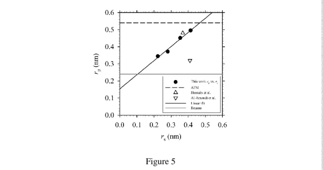
True retention versus flux values allow the fitting of the experimental results to the proposed nanofiltration model, providing the pore radius as the fitting parameter. Results of these fitted radii versus the corresponding solute Stokes radius are represented in Fig. 5 as solid black symbols. A linear increase of the predicted pore radius with the solute size is clearly observed. This goes in accordance with previous observations for other membranes and uncharged solutes [3]. For this case, linear
correlation relating both radii is:
r
p
0.826·
r
s
1.534·10
10
0.826·
r
s
0.54786·
d
w. Thislength dW could be interpreted as referring to the hydration layer of the pore walls that adds to that of the molecules of the solute.
1 2 3 4 5 6 7 8 9 10 11 12 13 14 15 16 17 18 19 20 21 22 23 24 25 26 27 28 29 30 31 32 33 34 35 36 37 38 39 40 41 42 43 44 45 46 47 48 49 50 51 52 53 54 55 56 57 58 59 60 61 62 63 64 65
-23-
[77]. For PEG-200 radius we have taken a value of 0.42 nm, as the average of two values found in the literature: rs(PEG-200)=0.41 nm [84] and rs(PEG-200)=0.43 nm [85]. This value is totally in agreement with our results if cylindrical pore geometry is assumed in the model. This value, although acceptable for pore size, does not correspond with the tendency shown in Fig. 5. This could be justified by the polydispersity of PEG-200, and the fact that the assumed pore geometry was not declared. The last value shown in Fig. 5 is 0.24 nm, an average reported by Boussu et al. from PALS (PositronAnnihilation Lifetime Spectroscopy) measurements [81, 86].
Figure 5
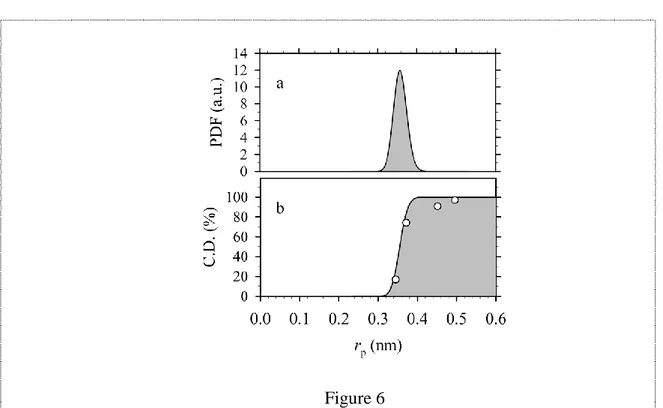
4.4. Pore size distribution.
Once pore radius is obtained as the fitting parameter of the model described in section 2, different two parameter distributions were tried to obtain the pore size distribution. These were: the normal, the log-normal, weibull, and logistic distributions. Good fit is obtained with all of them. As four results were quite similar, the differences between the means were below 0.3% and the maximum differences in standard deviation was 10%, only one will be presented, the log-normal distribution. This is found and justify in many other works[87], as those of Van der Bruggen and Vandecasteele [88], and because is the basis for some models [89].
2 2
1 2
ln /2
2
1 ( )
2
x a a
f x e
xa
1 2 3 4 5 6 7 8 9 10 11 12 13 14 15 16 17 18 19 20 21 22 23 24 25 26 27 28 29 30 31 32 33 34 35 36 37 38 39 40 41 42 43 44 45 46 47 48 49 50 51 52 53 54 55 56 57 58 59 60 61 62 63 64 65
-24-
The cumulative distribution of flux passing through the pores of different sizes can be obtained using Eq. (24). The distribution parameters are fitted using the four data for retention for the higher Jv for each solute. From the retention data we can obtain
Jw,t/Jw as a function of rp corresponding to all the solutes used. This cumulative distribution can be fitted to F(rp) functions and thus gives the differential distributions shown in Fig. 6. This graph shows the pore distribution obtained from the fit of non-charged retention measurement, for cylindrical pore geometry.
Boussu in his Ph.D. thesis indicates “The mean pore size represents the size of a molecule with 50% retention” [81]. From the present work retention measurement, for any pressure over 1 MPa, the true retention would be 0.5 if the solute size was between EG and DEG (as can be seen in Figs. 4 and 5). With data from Table 1 it is clear that this could be expected for a value between 0.22 and 0.28 nm; which corresponds with the result reported by Boussu, a value of 0.24 nm. However from pore size distribution this work estimates a little higher value, 0.35 nm.
Figure 6
4.5. Dependence with
1 2 3 4 5 6 7 8 9 10 11 12 13 14 15 16 17 18 19 20 21 22 23 24 25 26 27 28 29 30 31 32 33 34 35 36 37 38 39 40 41 42 43 44 45 46 47 48 49 50 51 52 53 54 55 56 57 58 59 60 61 62 63 64 65
-25-
transfer coefficient dependence; in this case, expressed by Eq. (17). The parameters in this relationship; i.e. A, and , depend on the experimental setting, regime, and even on membrane. The parameter is always taken as 1/3, but the value of value has been claimed to be from 0.65 up to 0.8. Figs. 7a and 7b show the dependence of the maximum retention and the estimated pore radius on the different possible values for α. In these plots, α-axis interval includes the range found in the literature. In the vicinity of
=0.75, a variation of , =0.1 produces a change in the pore radius estimation of 0.1
nm. In the literature, we found values for from 0.567 up to 0.8; this difference would represent a 60% change in the fitted pore radius.
For the retention values, identical changes in alpha, from 0.567 to 0.8, produce changes in the maximum retention of + 66% and - 10% for the case of EG retention, and + 17 % to -5 % in the case of DEG. Differences in pore radius due to small variation of α are even bigger that those from using different pore flow models [90].
1 2 3 4 5 6 7 8 9 10 11 12 13 14 15 16 17 18 19 20 21 22 23 24 25 26 27 28 29 30 31 32 33 34 35 36 37 38 39 40 41 42 43 44 45 46 47 48 49 50 51 52 53 54 55 56 57 58 59 60 61 62 63 64 65
-26- 5. Conclusions
The technique developed in this work allows the evaluation of the pore size distribution for a nanofiltration membrane. The use of neutral solutes permitted us to use a model that reduces solute-membrane interactions to size exclusion at the entrance of the pore and to the effects of internal friction. Note that the model assumes cylindrical pores and spherical solute molecules. The fact that these solutes were of very similar chemical nature causes the other effects, not taken into account in the mode, to have the same incidence for all solutes tested. This fact is illustrated with the linear relationship found between the Stokes radius of the solutes and the pore radius provided by the model for that solute. The comparison of our results with others found in the literature, obtained with a similar procedure or even with other techniques of different nature, show the validity of the data obtained.
Note, that for other ranges of filtration (for example MF and UF) pore radius measured using AFM technique is lower that the real one, due to the convolution of the tip with the sample. However, the applicability of AFM to estimate NF pore sizes is not so reliable; since pore sizes are even smaller than the tip point dimensions leading to overestimated pore sizes.
The type of function used to obtain the pore size distribution does not influence significantly on the characteristic values (mean and standard deviation) that this defines. Therefore, a distribution used traditionally as the log-normal can be a good choice to represent this type of data.
The influence of mass transfer, in fluid layers adjacent to the membrane surface in which the concentration and speed profile are developed, has been highlighted. Small changes in the correlation coefficient used to calculate the mass transfer coefficient produce important changes in the values of the distribution. For this reason a good method to obtain reliable concentrations over the surface of the membrane is essential to obtain the distribution of pore sizes in nanofiltration membranes with certain trustworthiness using this solute retention model.
1 2 3 4 5 6 7 8 9 10 11 12 13 14 15 16 17 18 19 20 21 22 23 24 25 26 27 28 29 30 31 32 33 34 35 36 37 38 39 40 41 42 43 44 45 46 47 48 49 50 51 52 53 54 55 56 57 58 59 60 61 62 63 64 65
-27-
1 2 3 4 5 6 7 8 9 10 11 12 13 14 15 16 17 18 19 20 21 22 23 24 25 26 27 28 29 30 31 32 33 34 35 36 37 38 39 40 41 42 43 44 45 46 47 48 49 50 51 52 53 54 55 56 57 58 59 60 61 62 63 64 65
-28- References
[1] A.W. Mohammad, Editorial: Nanofiltration membranes, Desalination, 315 (2013) 1. [2] S.-i. Nakao, Determination of pore size and pore size distribution: 3. Filtration membranes, Journal of Membrane Science, 96 (1994) 131-165.
[3] J.A. Otero, O. Mazarrasa, J. Villasante, V. Silva, P. Prádanos, J.I. Calvo, A. Hernández, Three independent ways to obtain information on pore size distributions of nanofiltration membranes, Journal of Membrane Science, 309 (2008) 17-27.
[4] J.A. Otero, R. Gutiérrez, I. Arnáez, P. Prádanos, L. Palacio, A. Hernández, Structural and functional study of two nanofiltration membranes, Desalination, 200 (2006) 354-355. [5] H. Grosse-Wilde, J. Uhlenbusch, Measurement of local mass-transfer coefficients by holographic interferometry, International Journal of Heat and Mass Transfer, 21 (1978) 677-682.
[6] C.L. Saluja, B.L. Button, B.N. Dobbins, Full-field in situ measurement of local mass transfer coefficient using ESPI with the swollen polymer technique, International Journal of Heat and Mass Transfer, 31 (1988) 1375-1384.
[7] J. Fernández-Sempere, F. Ruiz-Beviá, R. Salcedo-Díaz, Measurements by holographic interferometry of concentration profiles in dead-end ultrafiltration of polyethylene glycol solutions, Journal of Membrane Science, 229 (2004) 187-197.
[8] M.J. Fernandez-Torres, F. Ruiz-Bevia, J. Fernandez-Sempere, M. Lopez-Leiva, Visualization of the UF polarized layer by holographic interferometry, AIChE Journal, 44 (1998) 1765-1776.
[9] J. Fernández-Sempere, F. Ruiz-Beviá, R. Salcedo-Díaz, P. García-Algado, Measurement of Concentration Profiles by Holographic Interferometry and Modelling in Unstirred Batch Reverse Osmosis, Industrial & Engineering Chemistry Research, 45 (2006) 7219-7231. [10] D. Mahlab, N.B. Yosef, G. Belfort, Concentration polarization profile for dissolved species in unstirred batch hyperfiltration (Reverse Osmosis) - II Transient case, Desalination, 24 (1977) 297-303.
[11] D. Mahlab, N.B. Yosef, G. Belfort, Interferometric measurement of concentration polarization profile for dissolved species in unstirred batch hyperfiltration (reverse osmosis), Chemical Engineering Communications, 6 (1980) 225-243.
[12] J.C. Chen, Q. Li, M. Elimelech, In situ monitoring techniques for concentration polarization and fouling phenomena in membrane filtration, Advances in Colloid and Interface Science, 107 (2004) 83-108.
[13] S.S. Sablani, M.F.A. Goosen, R. Al-Belushi, M. Wilf, Concentration polarization in ultrafiltration and reverse osmosis: a critical review, Desalination, 141 (2001) 269-289. [14] V. Gekas, B. Hallström, Mass transfer in the membrane concentration polarization layer under turbulent cross flow : I. Critical literature review and adaptation of existing sherwood correlations to membrane operations, Journal of Membrane Science, 30 (1987) 153-170.
[15] X.-L. Wang, T. Tsuru, M. Togoh, S.-i. Nakao, S. Kimura, Evaluation of Pore Structure and Electrical Properties of Nanofiltration Membranes, Journal of Chemical Engineering of Japan, 28 (1995) 186-192.
[16] C. Combe, C. Guizard, P. Aimar, V. Sanchez, Experimental determination of four characteristics used to predict the retention of a ceramic nanofiltration membrane, Journal of Membrane Science, 129 (1997) 147-160.
[17] S. Déon, P. Dutournié, P. Bourseau, Modeling nanofiltration with Nernst-Planck approach and polarization layer, AIChE Journal, 53 (2007) 1952-1969.
1 2 3 4 5 6 7 8 9 10 11 12 13 14 15 16 17 18 19 20 21 22 23 24 25 26 27 28 29 30 31 32 33 34 35 36 37 38 39 40 41 42 43 44 45 46 47 48 49 50 51 52 53 54 55 56 57 58 59 60 61 62 63 64 65
-29-
[19] J.D. Ferry, Statistical evaluation of sieve constants in ultratiltration, The Journal of General Physiology, 20 (1936) 95-104.
[20] J.C. Giddings, E. Kucera, C.P. Russell, M.N. Myers, Statistical theory for the equilibrium distribution of rigid molecules in inert porous networks. Exclusion chromatography, The Journal of Physical Chemistry, 72 (1968) 4397-4408.
[21] P. Dechadilok, W.M. Deen, Hindrance Factors for Diffusion and Convection in Pores, Industrial & Engineering Chemistry Research, 45 (2006) 6953-6959.
[22] W.M. Deen, Hindered transport of large molecules in liquid-filled pores, AIChE Journal, 33 (1987) 1409-1425.
[23] W.L. Haberman, R.M. Sayre, Motion of rigid and fluid spheres in stationary and moving liquids inside cylindrical tubes, in: D.o.t. Navy (Ed.), Washington, 1958, pp. 70. [24] V. Silva, P. Prádanos, L. Palacio, A. Hernández, Alternative pore hindrance factors: What one should be used for nanofiltration modelization?, Desalination, 245 (2009) 606-613.
[25] V. Silva, P. Prádanos, L. Palacio, J.I. Calvo, A. Hernández, Relevance of hindrance factors and hydrodynamic pressure gradient in the modelization of the transport of neutral solutes across nanofiltration membranes, Chemical Engineering Journal, 149 (2009) 78-86.
[26] S. Déon, P. Dutournié, P. Fievet, L. Limousy, P. Bourseau, Concentration polarization phenomenon during the nanofiltration of multi-ionic solutions: Influence of the filtrated solution and operating conditions, Water Research, 47 (2013) 2260-2272.
[27] V. Geraldes, M.D. Afonso, Prediction of the concentration polarization in the nanofiltration/reverse osmosis of dilute multi-ionic solutions, Journal of Membrane Science, 300 (2007) 20-27.
[28] E. Nagy, Basic equations of the mass transport through a membrane layer, First ed., Elsevier, Amsterdam, 2012.
[29] E. Nagy, E. Kulcsár, A. Nagy, Membrane mass transport by nanofiltration: Coupled effect of the polarization and membrane layers, Journal of Membrane Science, 368 (2011) 215-222.
[30] H. Wijmans, Membrane Separations | Concentration Polarization, in: I.D. Wilson (Ed.) Encyclopedia of Separation Science, Academic Press, Oxford, 2000, pp. 1682-1687.
[31] S. Bandini, L. Bruni, Transport Phenomena in Nanofiltration Membranes, in: D. Enrico, G. Lidietta (Eds.) Comprehensive Membrane Science and Engineering, Elsevier, Oxford, 2010, pp. 67-89.
[32] G.B. Berg van den, I.G. Rácz, C.A. Smolders, Mass transfer coefficients in cross-flow ultrafiltration, Journal of Membrane Science, 47 (1989) 25-51.
[33] A. Escoda, S. Déon, P. Fievet, Assessment of dielectric contribution in the modeling of multi-ionic transport through nanofiltration membranes, Journal of Membrane Science, 378 (2011) 214-223.
[34] G. Jonsson, C.E. Boesen, Concentration polarization in a reverse osmosis test cell, Desalination, 21 (1977) 1-10.
[35] Z.V.P. Murthy, S.K. Gupta, Estimation of mass transfer coefficient using a combined nonlinear membrane transport and film theory model, Desalination, 109 (1997) 39-49. [36] N.A. Ochoa, P. Prádanos, L. Palacio, C. Pagliero, J. Marchese, A. Hernández, Pore size distributions based on AFM imaging and retention of multidisperse polymer solutes: Characterisation of polyethersulfone UF membranes with dopes containing different PVP, Journal of Membrane Science, 187 (2001) 227-237.
[37] M. Bakhshayeshi, A. Teella, H. Zhou, C. Olsen, W. Yuan, A.L. Zydney, Development of an optimized dextran retention test for large pore size hollow fiber ultrafiltration membranes, Journal of Membrane Science, 421–422 (2012) 32-38.
1 2 3 4 5 6 7 8 9 10 11 12 13 14 15 16 17 18 19 20 21 22 23 24 25 26 27 28 29 30 31 32 33 34 35 36 37 38 39 40 41 42 43 44 45 46 47 48 49 50 51 52 53 54 55 56 57 58 59 60 61 62 63 64 65
-30-
[39] G. Tkacik, S. Michaels, A Rejection Profile Test for Ultrafiltration Membranes & Devices, Nat Biotech, 9 (1991) 941-946.
[40] M.-H. Wang, A.N. Soriano, A.R. Caparanga, M.-H. Li, Mutual diffusion coefficients of aqueous solutions of some glycols, Fluid Phase Equilibria, 285 (2009) 44-49.
[41] E.D. Snijder, M.J.M. te Riele, G.F. Versteeg, W.P.M. van Swaaij, Diffusion coefficients of several aqueous alkanolamine solutions, J. Chem. Eng. Data, 38 (1993) 475-480.
[42] J. Fernández-Sempere, F. Ruiz-Beviá, J. Colom-Valiente, F. Más-Pérez, Determination of Diffusion Coefficients of Glycols, J. Chem. Eng. Data, 41 (1996) 47-48.
[43] L. Paduano, R. Sartorio, G. D'Errico, V. Vitagliano, Mutual diffusion in aqueous solution of ethylene glycol oligomers at 25 [degree]C, Journal of the Chemical Society, Faraday Transactions, 94 (1998) 2571-2576.
[44] R. Callendar, D. Leaist, Diffusion Coefficients for Binary, Ternary, and Polydisperse Solutions from Peak-Width Analysis of Taylor Dispersion Profiles, Journal of Solution Chemistry, 35 (2006) 353-379.
[45] J.M. Coulson, J.F. Richardson, J.R. Backhurst, J.H. Harker, Coulson & Richardson's Chemical Engineering, Sixth ed., Butterworth Heinemann, Oxford, 1999.
[46] R.H. Perry, D.W. Green, Perry's Chemical Engineers' Handbook (7th Edition), Seventh ed., McGraw-Hill, 1997.
[47] N.O. Becht, D.J. Malik, E.S. Tarleton, Evaluation and comparison of protein ultrafiltration test results: Dead-end stirred cell compared with a cross-flow system, Separation and Purification Technology, 62 (2008) 228-239.
[48] A. Mehta, A.L. Zydney, Effect of Membrane Charge on Flow and Protein Transport during Ultrafiltration, Biotechnology Progress, 22 (2006) 484-492.
[49] A.I. Schäfer, A.G. Fane, T.D. Waite, Nanofiltration Principles and Applications, First ed., Elsevier, Oxford, 2005.
[50] C.K. Colton, K.A. Smith, Mass transfer to a rotating fluid. Part II. Transport from the base of an agitated cylindrical tank, AIChE Journal, 18 (1972) 958-967.
[51] T.G. Kaufmann, E.F. Leonard, Studies of intramembrane transport: A phenomenological approach, AIChE Journal, 14 (1968) 110-117.
[52] P.H. Calderbank, M.B. Moo-Young, The continuous phase heat and mass-transfer properties of dispersions, Chemical Engineering Science, 16 (1961) 39-54.
[53] J. Marangozis, A.I. Johnson, A correlation of mass transfer data of solid-liquid systems in agitated vessels, The Canadian Journal of Chemical Engineering, 40 (1962) 231-237. [54] T.H. Chilton, A.P. Colburn, Mass Transfer (Absorption) Coefficients Prediction from Data on Heat Transfer and Fluid Friction, Industrial & Engineering Chemistry, 26 (1934) 1183-1187.
[55] E.R.G. Eckert, T.W. Jackson, Analysis of turbulent free-convection boundary layer on flat plate, in, NACA, 1951, pp. 255-261.
[56] R.W. Rousseau, Handbook of Separation Process Technology, in, John Wiley & Sons, 1987.
[57] W.F. Blatt, A. Dravis, A.S. Michaels, L. Nelson, Membrane Science and Technology: Industrial, Biological, and Waste Treatment Processes, Plenum Press, New York, 1970. [58] F.W. Dittus, L.M.K. Boelter, Heat transfer in automobile radiators of the tubular type, International Communications in Heat and Mass Transfer, 12 (1985) 3-22.
[59] R. Deissler, Analysis of turbulent heat transfer, mass transfer and friction in smooth tubes at high Prandtl and Schmidt numbers, in: J.P. Hartnett (Ed.) Advances in Heat and Mass Transfer, McGraw-Hill, New York, 1961.
[60] J.F. Richardson, J.H. Harker, J.R. Backhurst, Coulson & Richardson's Chemical Engineering, Fifth ed., Butterworth Heinemann, Oxford, 1995.
1 2 3 4 5 6 7 8 9 10 11 12 13 14 15 16 17 18 19 20 21 22 23 24 25 26 27 28 29 30 31 32 33 34 35 36 37 38 39 40 41 42 43 44 45 46 47 48 49 50 51 52 53 54 55 56 57 58 59 60 61 62 63 64 65
-31-
[62] S. Nicolas, B. Balannec, F. Beline, B. Bariou, Ultrafiltration and reverse osmosis of small non-charged molecules: A comparison study of rejection in a stirred and an unstirred batch cell, Journal of Membrane Science, 164 (2000) 141-155.
[63] G.H. Koops, S. Yamada, S.I. Nakao, Separation of linear hydrocarbons and carboxylic acids from ethanol and hexane solutions by reverse osmosis, Journal of Membrane Science, 189 (2001) 241-254.
[64] W.S. Opong, A.L. Zydney, Diffusive and convective protein transport through asymmetric membranes, AIChE Journal, 37 (1991) 1497-1510.
[65] A. Nora'aini, A. Wahab Mohammad, A. Jusoh, M.R. Hasan, N. Ghazali, K. Kamaruzaman, Treatment of aquaculture wastewater using ultra-low pressure asymmetric polyethersulfone (PES) membrane, Desalination, 185 (2005) 317-326.
[66] K.A. Smith, C.K. Colton, E.W. Merrill, L.B. Evans, Convective transport in a batch dialyzer: determination of true membrane permeability from a single measurement, AiChE Symp. Ser., 64 (1968) 45-58.
[67] A.L. Ahmad, L.S. Tan, S.R.A. Shukor, Modeling of the retention of atrazine and dimethoate with nanofiltration, Chemical Engineering Journal, 147 (2009) 280-286. [68] R.P. Schwarzenbach, P.M. Gschwend, D.M. Imboden, Second ed., John Wiley & Sons, Inc., 2005.
[69] G.E. Company, HL Series. Water Softening NF Elements. Fact Sheet, in: G.E. Company (Ed.), 2009.
[70] P. Eriksson, M. Kyburz, W. Pergande, NF membrane characteristics and evaluation for sea water processing applications, Desalination, 184 (2005) 281-294.
[71] K. Boussu, C. Kindts, C. Vandecasteele, B. Van der Bruggen, Applicability of nanofiltration in the carwash industry, Separation and Purification Technology, 54 (2007) 139-146.
[72] X. Wang, W. Liu, D. Li, W. Ma, Arsenic (V) removal from groundwater by GE-HL nanofiltration membrane: effects of arsenic concentration, pH, and co-existing ions, Frontiers of Environmental Science & Engineering in China, 3 (2009) 428-433.
[73] Y. Li, A. Shahbazi, K. Williams, C. Wan, Separate and Concentrate Lactic Acid Using Combination of Nanofiltration and Reverse Osmosis Membranes, Applied Biochemistry and Biotechnology, 147 (2008) 1-9.
[74] N. García-Martín, S. Perez-Magariño, M. Ortega-Heras, C. González-Huerta, M. Mihnea, M.L. González-Sanjosé, L. Palacio, P. Prádanos, A. Hernández, Sugar reduction in musts with nanofiltration membranes to obtain low alcohol-content wines, Separation and Purification Technology, 76 (2010) 158-170.
[75] N. García-Martín, S. Perez-Magariño, M. Ortega-Heras, M.L. González-Sanjosé, L. Palacio, P. Prádanos, A. Hernández, Sugar reduction in white and red musts with nanofiltration membranes, Desalination and Water Treatment, 27 (2011) 167-174.
[76] A. Al-Amoudi, P. Williams, S. Mandale, R.W. Lovitt, Cleaning results of new and fouled nanofiltration membrane characterized by zeta potential and permeability, Separation and Purification Technology, 54 (2007) 234-240.
[77] A. Al-Amoudi, P. Williams, A.S. Al-Hobaib, R.W. Lovitt, Cleaning results of new and fouled nanofiltration membrane characterized by contact angle, updated DSPM, flux and salts rejection, Applied Surface Science, 254 (2008) 3983-3992.
[78] D.R. Lide, CRC Handbook of Chemistry and Physics, 85 ed., CRC Press, Boca Raton, FL, 2005.
[79] A.A. Hussain, S.K. Nataraj, M.E.E. Abashar, I.S. Al-Mutaz, T.M. Aminabhavi, Prediction of physical properties of nanofiltration membranes using experiment and theoretical models, Journal of Membrane Science, 310 (2008) 321-336.