On a New Theoretical Framework for RR Lyrae Stars. II.
Mid-infrared Period
–
Luminosity
–
Metallicity Relations
Jillian R. Neeley1, Massimo Marengo1, Giuseppe Bono2,3, Vittorio F. Braga2,3,4,5,6, Massimo Dall’Ora7, Davide Magurno2,3, Marcella Marconi7, Nicolas Trueba1, Emanuele Tognelli8,9, Pier G. Prada Moroni8,9, Rachael L. Beaton10, Wendy L. Freedman11,
Barry F. Madore10, Andrew J. Monson12, Victoria Scowcroft13, Mark Seibert10, and Peter B. Stetson14 1
Department of Physics & Astronomy, Iowa State University, Ames, IA 50011, USA;[email protected] 2
Department of Physics, Università di Roma Tor Vergara, via della Ricerca Scientifica 1, I-00133 Roma, Italy
3
INAF-Osservatorio Astronomico di Roma, via Frascati 33, I-00040 Monte Porzio Catone, Italy
4
ASDC, via del Politecnico snc, I-00133 Roma, Italy
5
Departamento de Fisica, Universidad Andres Bello, Av. Fernandez Concha 700, Las Condes, Santiago, Chile
6
Instituto Milenio de Astrofisica, Santiago, Chile
7
INAF-Osservatorio Astronomico di Capodimonte, Salita Moiarello 16, I-80131 Napoli, Italy
8
Dipartimento di Fisica, Università di Pisa, Lago Bruno Pontecorvo 3, I-56127, Pisa, Italy
9
INFN, Sezione di Pisa, Lago Bruno Pontecorvo 3, I-56127, Pisa, Italy
10
Carnegie Observatories, 813 Santa Barbara Street, Pasadena, CA 91101, USA
11
Department of Astronomy & Astrophysics, University of Chicago, Chicago, IL 60637, USA
12Department of Astronomy & Astrophysics, The Pennsylvania State University, 525 Davey Lab, University Park, PA 16802, USA 13
Department of Physics, University of Bath, Claverton Down, Bath BA2 7AY, UK
14
NRC-Herzberg, Dominion Astrophysical Observatory, 5071 West Saanich Road, Victoria BC V9E 2E7, Canada
Received 2017 March 3; revised 2017 May 2; accepted 2017 May 3; published 2017 May 26
Abstract
We present new theoretical period–luminosity–metallicity(PLZ) relations for RR Lyræ stars(RRLs)at Spitzer and WISE wavelengths. The PLZ relations were derived using nonlinear, time-dependent convective hydrodynamical models for a broad range of metal abundances(Z=0.0001–0.0198). In deriving the light curves, we tested two sets of atmospheric models and found no significant difference between the resulting mean magnitudes. We also compare our theoretical relations to empirical relations derived from RRLs in both thefield and in the globular cluster M4. Our theoretical PLZ relations were combined with multi-wavelength observations to simultaneously fit the distance modulus,μ0, and extinction,AV, of both the individual Galactic RRL and of the cluster M4. The results for the Galactic
RRL are consistent with trigonometric parallax measurements fromGaia’sfirst data release. For M4, wefind a distance modulus ofμ0=11.257±0.035 mag withAV=1.45±0.12 mag, which is consistent with measurements from other distance indicators. This analysis has shown that, when considering a sample covering a range of iron abundances, the metallicity spread introduces a dispersion in the PL relation on the order of 0.13 mag. However, if this metallicity component is accounted for in a PLZ relation, the dispersion is reduced to∼0.02 mag at mid-infrared wavelengths. Key words:infrared: stars –stars: horizontal-branch– stars: variables: RR Lyrae
Supporting material:machine-readable tables
1. Introduction
RR Lyræ(RRL)variables are a popular tracer for old stellar populations, thanks to their abundance in the globular clusters, halos, and bulges of galaxies (see e.g., Vivas & Zinn 2006; Dékány et al. 2013; Pietrukowicz et al. 2015). During their advanced evolutionary phases low- and intermediate-mass stars cross the so-called Cepheid instability strip(a region of the HR diagram in which stellar atmospheres are pulsationally stable). Unlike their higher-mass counterparts, RRLs do not appear to obey well defined period–luminosity (PL) relations at visible wavelengths. As a consequence, their usefulness as distance indicators has been historically limited to the adoption of a luminosity–metallicity relation characterized by a rather large (≈5%)intrinsic scatter(Cáceres & Catelan2008). This relation also suffers from evolutionary effects and uncertainties related to the metallicity scale and/or αenhancement. Moreover, the relation is possibly nonlinear across the whole observed RRL metallicity range(Caputo et al.2000).
Several theoretical and empirical arguments, however, indicate that RRLs become solid distance indicators when moving from the optical to the infrared bands. As described as length in Bono et al.(2016), the main reasons are three-fold.
1. As first demonstrated over 30 years ago by Longmore et al. (1986) and again by Dall’Ora et al. (2004), an obvious PL relation does appear moving from the optical to the infrared bands. While the slope is vanishingly small in the V band, it becomes steeper with increasing wavelength (Catelan et al. 2004; Marconi et al. 2015), ranging from−1.2 in theRband to−2.2 in theKband. This behavior is different than the one shown by Cepheids(Bono et al.1999)and is related to the specific dependence of the RRL bolometric correction with temperature (Bono et al. 2001, 2003; Bono 2003). For λ2.2μm the slope of the PL relations of instability strip pulsators (both Cepheids and RRLs) becomes almost constant. In this wavelength regime the brightness variations of pulsating stars is mainly driven by their radius variation, and the effective temperature variations only play a minimal role (Jameson 1986; Madore & Freedman2012).
2. The intrinsic dispersion of the RRL PL relations steadily decreases when moving from the optical to the infrared bands. This trend is due to the fact that starting from the near-infrared (NIR) cooler RRLs are steadily brighter
The Astrophysical Journal,841:84(19pp), 2017 June 1 https://doi.org/10.3847/1538-4357/aa713d © 2017. The American Astronomical Society. All rights reserved.
than hotter ones, due to the stronger temperature sensitivity of the bolometric correction (Bono 2003). As a consequence, infrared PL relations are only marginally affected by the intrinsic width in temperature of the instability strip, since they almost mimic a PL–color relation. Furthermore, the instability strip itself becomes narrower at longer wavelengths and, as a consequence, the color term responsible for the intrinsic dispersion on the PL relations vanishes(Catelan et al.2004; Madore & Freedman2012; Marconi et al.2015). This means that at mid-infrared(MIR)wavelengths PL relations provide for more precise distance indicators(Braga et al.2015). 3. Infrared observations are less affected by reddening, due
to the power-law dependence of the extinction laws(λ−β, with β∼1.6 to 1.8; Bono et al. 2016). This translates into a smaller uncertainty of reddening and differential reddening, when compared to the V band, by a factor ranging from four(J)to ten(K). In theL- and M-band extinction is further reduced, reaching its minimum values with AV/Aλ≈15 and 20, respectively. This is a huge advantage when inspecting highly and differentially reddened targets, such as those in the Galactic bulge (Nishiyama et al.2009).
To explore the detailed physics behind these remarkable properties, Marconi et al. (2015)used new, time- and metal-dependent convective hydrodynamic models to derive a theoretical calibration for the period–luminosity–metallicity (PLZ), period–Wesenheit–metallicity (PWZ), and metal-inde-pendent period–Wesenheit (PW) relations of RRLs. These relations have been published in the optical (Johnson–Kron– Cousins’sBV RI)and NIR(2MASSJHK)wavelength regimes (Marconi et al.2015), and tested byfitting average magnitudes of RRLs in the M4 (NGC 6121) Galactic globular cluster (Braga et al. 2015)and in the dwarf spheroidal galaxy Carina (Coppola et al.2015). On the other hand, similar analysis in the MIR, where the extinction is lower and the intrinsic temperature-dependent scatter is at its smallest, is lagging. Several authors(Klein et al.2011; Madore et al.2013; Neeley et al. 2015) have derived empirical calibrations for Galactic RRL MIR PL relations, but their zero point calibration is based on just five stars for which ≈10% accuracy Hubble Space Telescope (HST) Fine Guidance Sensor (FGS) parallaxes are available(Benedict et al.2011). A detailed theoretical analysis of RRL PLZ relations in the MIR is lacking. Tofill this gap we decided to extend the detailed investigation of RRL pulsation properties provided by Marconi et al. (2015) to derive a theoretical calibration of RRL PLZ and PWZ relations in the MIR. In this paper we focus on the MIR bands available to the InfraRed Array Camera(IRAC, Fazio et al.2004)onboard theSpitzer Space Telescope(Werner et al.2004), as well as the passbands of the Wide-field Infrared Survey Explorer (WISE, Wright et al.2010).
Our choice offilters is motivated by two factors. First, both IRAC and WISE provide a large archive of Galactic and extragalactic observations with thousands of RRLs observed in one or multiple epochs. These include the “warm” Spitzer observational campaign of the Carnegie RR Lyrae Program (CRRP; Freedman et al.2012)and theSpitzerMerger History and Shape of the Halo program (SMHASH; Johnston et al.
2013), designed to obtain multi-epoch light-curves of RRLs in the halo and bulge of the Milky Way, as well as in dwarf galaxies and tidal streams. Second, the wavelength range
covered by IRAC and WISEwill be available as part of the James Webb Space Telescope (JWST) Near Infrared Camera (NIRCam) and the Mid-infrared Instrument imagers. The NIRCam wide filters F356W and F444W, in particular, are analogous to the IRAC warm passbands at 3.6 and 4.5μm. The predicted sensitivity of these twofilters(13.8 and 24.5 nJy for F356W and F444W for a 10σ detection in 10,000 s integration15) will allow the detection of RRLs at a distance modulus as high as ∼26 mag (1.6 Mpc), thereby covering a significant portion of the Local Group, at least in galaxies where the∼0.2 arcsec resolution will be sufficient to overcome confusion. This will open the possibility of using RRL distances to precisely calibrate secondary distance indicators independently from Cepheids, with the goal of providing a Population II route to the cosmological distance scale(Beaton et al.2016).
A detailed description of the models and the procedure we followed to derive the PLZ and PWZ relations in the IRAC and WISEbands are presented in Section2. To test the reliability of our theoretical relations in providing accurate distance estimates of individual stars, we have collected average magnitudes for a sample of Galactic RRLs with a broad range of metallicity, as well as revised our previously published photometry for the RRLs in the globular cluster M4. These observations are presented in Section 3. We compare our theoretical PLZ relations to empirical PL and PLZ relations from the literature in Section 4. In Sections 5 and 6 we use our synthetic PLZ relations tofit new distance moduli and visual band extinctions for Galactic and M4 RRLs, respectively, and compare these results to other estimates. The conclusions of our work, with a focus on the dependence of the PLZ relations on metallicity, are presented in Section7.
2. Theoretical Framework
Theoretical models allow us to derive new theoretical MIR PLZ relations, by adopting the same models and following the same steps described in Marconi et al.(2015). For a detailed discussion on the models, see Section2 of the quoted paper. Here, we want to stress only a few major points.
1. The models span a large range in metallicity. Seven different values of Z ranging from 0.0001 to 0.0198 (α-enhanced chemical mixture)are taken into account. 2. For each metallicity, either two or three luminosity levels
are included for fundamental(FU)or first overtone(FO) pulsators, to take into account evolved RRLs that are brighter than the zero-age horizontal branch (ZAHB). The three possible luminosity levels are logLZAHB (A),
L
log ZAHB+0.1(B), andlogLZAHB+0.2 with mass 10% lower than the other models(C).
3. The effective temperatures range between 7200 (bluest model on the ZAHB)and 5300 K (reddest model of the brightest luminosity level) with steps of 100 K. The individual A, B, and C sequences include from four to eleven FU models and from two to seven FO models. This range covers the temperature width of the instability strip.
In Marconi et al.(2015)we transformed the bolometric light curves of the quoted grid into the 2MASS JHK and theUBVRI photometric bands using the bolometric corrections(BCs)and
15
http://www.stsci.edu/jwst/instruments/nircam/sensitivity/table
2
color–temperature relations obtained from the synthetic spectra provided by Castelli & Kurucz(2004). To transform the same models into the IRAC16and theWISE17photometric bands, we decided to perform a test to estimate the impact that different sets of synthetic spectra have on MIR bands. In particular, we used the atmosphere models provided by Brott & Hauschildt (2005) (covering 2700 K < Teff < 10,000 K and -0.5
g
log 0.5) and by Castelli & Kurucz (2004) (covering 3500 K < Teff < 50,000 K and 0.0logg5.0). The
adopted synthetic spectra are available for a wide range of [Fe/H], namely for −4.0 < [Fe/H] < +0.5. The Brott & Hauschildt(2005)spectra are also available for several[α/Fe] values in [−0.2, +0.8] with a spacing of 0.2 dex, while the Castelli & Kurucz(2004)ones are computed only for[α/Fe]= 0.0 and +0.4. For present calculations we adopted the spectra with [α/Fe] = +0.4 in both cases. Since the two spectral libraries adopt different assumptions concerning the solar abundances(Brott & Hauschildt2005adopted the Grevesse & Noels1993solar abundances whereas Castelli & Kurucz2004
adopted those from Grevesse & Sauval1998), we placed them on the same scale by converting the [Fe/H]of each synthetic spectrum into the total metallicity Z. The relation used for this conversion islog(Z X)-log(Z X)=[Fe H]+0.35
wherelog(Z X)= -1.61(Pietrinferni et al.2006). We obtained the BCs for all the Teff,logg and [Fe/H](Z)
values available in the spectral library. Then, we computed the magnitudes by interpolating the BC tables at the requestedTeff,
g
log and total metallicityZalong each bolometric light curve. The transformations were computed for the two different sets of atmosphere models and we found that the difference is negligible. Data plotted in Figure1 display that the difference
in MIR mean magnitudes ranges from a few thousandths close to the blue (hot) edge of the instability strip to at most one hundredth of a magnitude close to the red (cool) edge of the instability strip. Data plotted in thisfigure refer to a sequence of FU models constructed atfixed mass, luminosity, and chemical composition (see labeled values). However, the difference is minimal over the entire grid of models. For the above reasons, and for homogeneity with previous predictions, we decided to use the BC and the CT relations provided by Castelli & Kurucz(2004).
Finally, we fitted the periods, mean magnitudes, and metallicities—now transformed into iron abundances—and obtained the coefficients of the PLZ relations. The mean magnitudes for the entire grid of models are given in Tables1
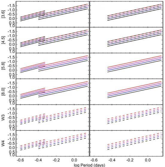
and 2 for the FO and FU pulsators respectively. The coefficients are given in Table 3, and the relations for four metallicities ([Fe/H] from 0 to −3.0 dex) are plotted in Figure 2. Preliminary results based on two different metal abundances and three different helium contents indicate that pulsation properties of RRLs are minimally affected by the helium content. The key variation between models with canonical and enhanced helium content is the luminosity, and in turn the pulsation period (Marconi et al. 2011). A more detailed investigation will be addressed in a forthcoming paper (M. Marconi et al. 2017, in preparation), where the entire grid of model light curves, from the optical to MIR bands and covering the entire range in metallicity and helium abundance of RRLs, will also be published.
We also obtained the coefficients for two- and three-band PWZ relations, where the Wesenheit magnitude is defined as W B B( 1, 2)=MB1-a(MB1-MB2)orW B B( 1, 2,B3)=MB1
-MB2 MB3
a( - ). The coefficients of the color term,α, werefixed according to the reddening law we have adopted (Cardelli et al.1989). The coefficients for the color term and the PWZ relations are given in Tables4 and 5 for two- and three-band PWZ. For readers interested in the coefficients of the PWZ Figure 1.Top: difference in[4.5]magnitudes as a function of the effective temperature for a set of FU models computed atfixed stellar mass(0.716Me), luminosity
(logL L=1.72), and chemical composition(Z=0.0003,Y=0.245). Bolometric light curves predicted by hydrodynamical pulsation models were transformed into the observational plane by using color–temperature relations provided by Castelli & Kurucz(2004)and by Brott & Hauschildt(2005).Teffspans the range between the blue and red edge of the instability strip. Bottom: same as the top, but for the[3.6]magnitudes.
16
Transmission curves for IRAC available at: http://irsa.ipac.caltech.edu/ data/SPITZER/docs/irac/calibrationfiles/spectralresponse/.
17
Transmission curves forWISEavailable at: http://wise2.ipac.caltech.edu/
docs/release/prelim/expsup/sec4_3g.html.
3
relation assuming a different reddening law, we provide a Python program,18in which one can input the coefficients(Aλ/ AV) of an alternative reddening law, and it will output the
corresponding coefficients of the PWZ relation. The full versions of Tables 1, 2, 4, and5 are available in the online journal and portions are shown here for form and content.
By comparing the results described above with those obtained by Marconi et al.(2015)in their Table6, we outline that (i) The dispersion of the relations is constant (within 0.01 mag)in the wavelength range from theHto theW4 band, with values of the order of σFO=0.02 mag, σFU =
0.03–0.04 mag and σFO+FU=0.04 mag. (ii) The metallicity coefficient shows no significant wavelength dependence from the Rto the IRAC bands, and is mainly due to the change in luminosity. This is because the metallicity dependence of the BCs effectively cancels out the change in Teff, resulting in a
minimal change in color (∼0.01 mag or less over the entire [Fe/H]range)as metallicity is increased.
3. Optical, NIR, and MIR Data
To test the model PLZ relations described in Section2, we compiled multi-wavelength observations for a sample of 55 nearby Galactic RRLs. The sample was based on stars included in the Hipparcos catalog, limited to stars with V<11 mag, AV<0.5, and an expected final Gaia parallax with 2%–3% accuracy. Most of the observations were collected as part of the Carnegie RR Lyrae Program (CRRP, PID 90002), and were published in Monson et al. (2017). The pulsation period, metallicity, extinction, and available distance moduli of the stars in our sample are listed in Table 6. In addition to the Galactic sample, we compiled observations of RRLs in the globular cluster M4. All data have been homogenized to the following photometric system: Kron–Cousins RI, 2MASS JHKs, SpitzerS19.2 3.6 and 4.5μm, Spitzer S18.25 5.8 and
Table 1
Intensity Mean Magnitudes for Entire Grid of FO Models
Te logL logP [3.6] [4.5] [5.8] [8.0] W1 W2 W3 W4
Z=0.0001Y=0.245M=0.80Me
7200 1.7600 −0.5088 −0.381 −0.385 −0.388 −0.393 −0.379 −0.385 −0.399 −0.415
7100 1.7600 −0.4901 −0.426 −0.430 −0.434 −0.439 −0.424 −0.431 −0.445 −0.461
7000 1.7600 −0.4703 −0.475 −0.479 −0.483 −0.488 −0.473 −0.479 −0.495 −0.510
6900 1.7600 −0.4495 −0.525 −0.529 −0.533 −0.538 −0.522 −0.529 −0.544 −0.560
6800 1.7600 −0.4282 −0.574 −0.578 −0.582 −0.587 −0.573 −0.579 −0.595 −0.611
6700 1.7600 −0.4077 −0.622 −0.626 −0.630 −0.636 −0.621 −0.627 −0.643 −0.660
6600 1.7600 −0.3855 −0.669 −0.673 −0.678 −0.682 −0.667 −0.674 −0.690 −0.707
7100 1.8600 −0.4093 −0.679 −0.683 −0.687 −0.692 −0.677 −0.683 −0.698 −0.714
7000 1.8600 −0.3891 −0.726 −0.730 −0.734 −0.739 −0.723 −0.730 −0.746 −0.762
6900 1.8600 −0.3691 −0.774 −0.779 −0.783 −0.788 −0.772 −0.779 −0.794 −0.811
6800 1.8600 −0.3472 −0.823 −0.828 −0.832 −0.837 −0.821 −0.828 −0.844 −0.860
6700 1.8600 −0.3261 −0.872 −0.877 −0.881 −0.887 −0.870 −0.877 −0.893 −0.910
(This table is available in its entirety in machine-readable form.)
Table 2
Intensity Mean Magnitudes for Entire Grid of FU Models
Te logL logP [3.6] [4.5] [5.8] [8.0] W1 W2 W3 W4
Z=0.0001Y=0.245M=0.80Me
6800 1.7600 −0.3016 −0.570 −0.574 −0.578 −0.584 −0.567 −0.574 −0.590 −0.607
6700 1.7600 −0.2795 −0.624 −0.628 −0.633 −0.638 −0.621 −0.629 −0.645 −0.662
6600 1.7600 −0.2574 −0.677 −0.682 −0.686 −0.692 −0.675 −0.682 −0.699 −0.716
6500 1.7600 −0.2358 −0.730 −0.734 −0.739 −0.745 −0.727 −0.734 −0.751 −0.769
6400 1.7600 −0.2124 −0.781 −0.785 −0.790 −0.796 −0.778 −0.785 −0.803 −0.821
6300 1.7600 −0.1892 −0.829 −0.833 −0.838 −0.844 −0.826 −0.834 −0.851 −0.870
6200 1.7600 −0.1650 −0.872 −0.877 −0.882 −0.888 −0.869 −0.877 −0.895 −0.914
6100 1.7600 −0.1421 −0.912 −0.917 −0.921 −0.928 −0.909 −0.917 −0.935 −0.954
6000 1.7600 −0.1178 −0.944 −0.949 −0.954 −0.960 −0.941 −0.949 −0.968 −0.987
6900 1.8600 −0.2389 −0.765 −0.770 −0.774 −0.779 −0.763 −0.770 −0.786 −0.802
6800 1.8600 −0.2180 −0.819 −0.824 −0.828 −0.834 −0.816 −0.824 −0.840 −0.857
6600 1.8600 −0.1744 −0.928 −0.932 −0.936 −0.942 −0.924 −0.932 −0.949 −0.966
6400 1.8600 −0.1282 −1.029 −1.034 −1.039 −1.045 −1.026 −1.034 −1.052 −1.070
6200 1.8600 −0.0813 −1.122 −1.128 −1.132 −1.139 −1.119 −1.128 −1.146 −1.164
6100 1.8600 −0.0567 −1.166 −1.172 −1.177 −1.183 −1.163 −1.172 −1.190 −1.209
6000 1.8600 −0.0334 −1.206 −1.212 −1.217 −1.223 −1.203 −1.212 −1.231 −1.250
5900 1.8600 −0.0088 −1.240 −1.246 −1.251 −1.258 −1.237 −1.246 −1.265 −1.284
(This table is available in its entirety in machine-readable form.)
18
Available athttps://github.com/jrneeley/Theoretical-PWZ-Relations.
4
8.0μm, andWISE W1,W2 andW3(see Monson et al.2017for details).
3.1. Galactic RRLs
The RIJHK data set was built from three sources: Monson et al.(2017), Klein (2014).19and Feast et al.(2008). The data set from Monson et al.(2017)combines observations collected for CRRP with the Three-hundred Millimeter telescope with archival observations from individual studies(and places them on a homogeneous photometric system), and was used as the basis for our sample of Galactic RRLs. For stars without multi-epoch observations in this data set, we supplemented with the multi-epoch observations available in Klein (2014). Light curves from Klein (2014)were obtained with the Nickel 1 m telescope at Lick Observatory and 1.3 m PAIRITEL telescope at the Fred Lawrence Whipple Observatory and were fit with Fourier series. Finally, Feast et al.(2008)presented a procedure to estimate mean magnitudes from single epoch 2MASS JHK measurements of RRLs. For any stars still missing multi-epoch JHKobservations from the previous two data sets, we adopted the estimated mean magnitude from Feast et al. (2008). The Feast et al. (2008) templates are not very precise, and we derived a single uncertainty for each band according to the standard deviation of the residuals between the template mean magnitude and derived mean magnitude of stars for which we have well sampled light curves. This results in uncertainties in the adopted mean magnitudes of 0.06, 0.04, and 0.07 mag for JHK, respectively.
MIR observations for our sample are also presented in Monson et al. (2017), which combined the Spitzer 3.6 and 4.5μm observations obtained for CRRP with WISE photo-metry. Thefirst two bands in theWISEphotometric system are
very similar to the IRAC bands, but we elected to keep the WISE and IRAC photometry separate in this paper for two main reasons. First, for most of the stars in our sample, adding in WISE photometry degrades the quality of our IRAC light curves(Figure3compares the quality ofWISEand IRAC light curves side by side). Second, the WISEand IRAC passbands are not identical, and it is unclear if there is an offset between the two calibrations. When comparing the average magnitudes of RRLs obtained withSpitzerandWISE, Monson et al.(2017)
saw a small offset. However, the AllWISE explanatory supplement20 found no offset with the first two IRAC bands. Given this unresolved discrepancy, we re-derived the average magnitudes separately for the IRAC andWISEdata presented in Monson et al.(2017). The IRAC light curves are covered by a minimum of 24 epochs over a single pulsation cycle(some stars were observed with up to 134 epochs to fill gaps in Spitzer’s schedule). We note that the Spitzer Science Center (SSC) recently released thefinal calibration of warm mission Spitzer data (S19.2). The new calibration included new flux conversions, linearity solution for the 3.6μm band, and flat fields, and is now consistent with the final cryogenic mission calibration(S18.25)defined by Carey et al.(2012). TheWISE photometry comes from the AllWISE data release, and provides an average of 36, 36, and 18 random epochs in the W1,W2, andW3 bands, respectively.
The GLOESS method (Neeley et al. 2015; Monson et al.
2017, and references therein) was used to fit smoothed light curves and derive the mean intensity magnitude in each of the bands. For stars in common with the CRRP sample, we found no significant difference in the mean magnitudes fit with Fourier series(Klein2014)and the GLOESS method(Monson et al.2017). Thefinal count for each band is as follows: 32 in Table 3
Theoretical NIR and MIR Period–Luminosity Relations for RR Lyrae
Filtersa a b c σ a b c σ a b c σ
±0.022 ±0.044 ±0.004 ±0.007 ±0.021 ±0.004 ±0.007 ±0.017 ±0.003
Notes.
The periods of FO variables were fundamentalized with the relation:logPF=logPFO+0.127.
19
Available online at:http://w.astro.berkeley.edu/∼cklein/dissertation.pdf.
20
Available online at: http://wise2.ipac.caltech.edu/docs/release/allwise/
expsup/.
5
R, 55 inI, 54 inJ, 53 inH, 54 inK, 51 in[3.6], 51 in[4.5], 55 inW1, 55 inW2, and 54 inW3.
3.2. M4 RRLs
Photometry for the RRLs in the globular cluster M4 is presented in Stetson et al.(2014) (RIJHK)and in Neeley et al. (2015) (Spitzer [3.6] and [4.5]). The RIJHK data were assembled from ∼65 data sets mostly taken at the VLT. The IRAC 3.6 and 4.5μm photometry presented in Neeley et al. (2015)was collected as part of CRRP, and has been updated in
this paper to the most recent Spitzer calibration (S19.2) using the same calibration procedure as for the Galactic RRLs. All photometry was undertaken using the DAOPHOT/ ALLSTAR/ALLFRAME(Stetson1987,1992,1994)suite of programs.
For this work, we have also performed new photometry of single-epoch archival observations of M4 from Spitzer’s cryogenic mission 5.8 and 8.0μm bands. The cluster was observed with a medium-scale 11-point cycling dither pattern, with a frame time of 100 s. Aperture photometry was performed on Basic Calibrated Data (BCD)generated by the Figure 2.Predicted RRL period–luminosity–metallicity relations for IRAC(solid lines)andWISE(dashed lines)bands. Left panels show separate RRc and RRab relations, while the right panels show the fundamentalized relations. Four metallicities are plotted:[Fe/H]=0(bottom black line),[Fe/H]=−1.0(blue line),
[Fe/H]=−2.0(purple line), and[Fe/H]=−3.0(top red line).
Table 4
Theoretical Two-band Period–Wesenheit–Metallicity Relations
Filtersa α a b c σ a b c σ a b c σ
FO FU FU+FO
I1,I–I1 0.126 −1.437 −2.784 0.154 0.018 −0.882 −2.354 0.186 0.030 −0.884 −2.343 0.182 0.032 ±0.020 ±0.039 ±0.003 ±0.006 ±0.018 ±0.003 ±0.006 ±0.015 ±0.003
I2,I–I2 0.094 −1.419 −2.770 0.154 0.018 −0.848 −2.319 0.193 0.032 −0.852 −2.306 0.187 0.034 ±0.021 ±0.041 ±0.003 ±0.007 ±0.019 ±0.003 ±0.006 ±0.016 ±0.003
Note. a
I1,I2,I3, andI4 correspond to IRAC 3.6μm, 4.5μm, 5.8μm, and 8.0μm, respectively. (This table is available in its entirety in machine-readable form.)
6
S18.25 pipeline with a 3-3-7 pixel aperture, and calibrated to the photometric system defined by Carey et al. (2012). The aperture corrections used were 1.1356 and 1.2255 at 5.8 and 8.0μm respectively. Photometry at the 11 dither positions was averaged to obtain a single measurement. These observations were obtained eight years before the CRRP Spitzer observa-tions, and we were unable to reliably determine the pulsation phase and construct a template to estimate the mean magnitude. Therefore we elected to use the single epoch observation as the estimated mean magnitude with an uncertainty equal to half the amplitude in the 3.6 or 4.5μm bands. These results as well as the updated mean magnitudes from Neeley et al. (2015) are available in Table 7.
4. Empirical PL Relations
We can directly compare our synthetic PLZ relations with some recent empirical relations. Since many empirical measurements have been made on single-metallicity popula-tions(i.e., in globular clusters), the metallicity component has not been reliably measured and only PL relations are available. One exception to this is the empirical PLZ relation in theW1 and W2 bands measured using several globular clusters (Dambis et al.2014). Both the period slope and the zero point are consistent between the theoretical and empirical methods. However the metallicity term they measure(0.096 mag/dex in W1 and 0.108 mag/dex inW2)is smaller than in our synthetic PLZ relations by about 4σ, but we note that their method is reliant on the accuracy of the visual band magnitude– metallicity relation. Madore et al. (2013) also measured PL relations in the WISE bands, but using only four RRab stars with parallax measurements. Due to their limited sample, the uncertainties on their derived parameters are very large (±0.9 mag in slope, ±0.2 mag in the zero point), and they were not able to see a metallicity dependence(these four stars also cover an extremely limited range in[Fe/H]).
We have recently completed a multi-wavelength analysis of the PL relation for the globular cluster M4(NGC 6121). The RIJHK relations were presented in Braga et al. (2015) and IRAC 3.6 and 4.5μm relations were originally presented in Neeley et al. (2015). For consistency, we have updated the calibrated relations from Neeley et al.(2015)to the newSpitzer S19.2 calibration, as well as extended the relations to the 5.8 and 8.0μm bands. The new FO, fundamental, and fundamen-talized relations are given in Table8. For the 3.6 and 4.5μm bands, the slope wasfixed using the cluster RRLs, and the zero point was determined using five Galactic RRLs(RR Lyr, RZ Cep, SU Dra, UV Oct, and XZ Cyg)with geometric parallaxes measured using the HST FGS (Benedict et al. 2011). The σ
quoted is the dispersion of the cluster RRLs around the PL relation. The fundamentalized calibrated relations result in a distance modulus of μ0=11.353±0.095 at 3.6μm and μ0=11.363±0.095 at 4.5μm, assuming extinction values calculated specifically for M4 (AV=1.39±0.01 and RV=3.62)in Hendricks et al.(2012). For the longer 5.8 and
8.0μm bands, the slope is based on single epoch photometry of the M4 RRL, so the uncertainties and dispersion are significantly larger. In addition, no photometry of the five calibrating RRLs was available in these bands, so the calibrated zero point is determined by applying the average distance modulus measured from the 3.6 and 4.5μm bands to the apparent zero point.
A comparison between the period dependence derived from theoretical methods and the empirical methods described above is shown in Figure 4. The theoretical period dependence is shown asfilled circles, and empirically derived slopes are over-plotted according to the legend. Overall the predicted period dependence in all bands is consistent with results from the literature, and we do observe the predicted flattening of the period dependence at longer wavelengths. The observed slope of the PL relation in M4 is within 1σ of the predicted slope in theJ,K, and IRAC bands. In the R,I and Hbands, the slope of the observed PL relations differs from the predicted relation by 2, 2.7, and 2σrespectively. This discrepancy could be due to the larger scatter in the PL relation at shorter wavelengths, but we note that wefind a better agreement with the synthetic HB-based slopes by Catelan et al.(2004)in these bands. Ongoing work on more globular clusters in the CRRP sample will help to better characterize the period dependence in the RRL PLZ relation.
5. Galactic RRL Distances
In addition to simply comparing theoretical and empirical results, we can use our synthetic PLZ relations to fit the data and obtain predicted distance moduli and extinctions for all of the RRLs in our sample. We used the synthetic PLZ relations to obtain predicted absolute magnitudes, Mλ, in the RIJHK, IRAC, and WISE bands. From these predicted absolute magnitudes, reddened distance moduli(ml-Ml)were calcu-lated, and then used in combination with a universal reddening law tofit both the true distance modulus(μ0)and visual band
extinction(AV)of each star using a weighted least-squaresfit of
the form
ml-Ml=m0+AV(A Al V) ( )1
where Aλ/AV are the coefficients of the reddening law. This
technique wasfirst introduced by Freedman et al.(1985,1991)
Table 5
Theoretical Three-band Period–Wesenheit–Metallicity Relations
Filtersa α a b c σ a b c σ a b c σ (This table is available in its entirety in machine-readable form.)
7
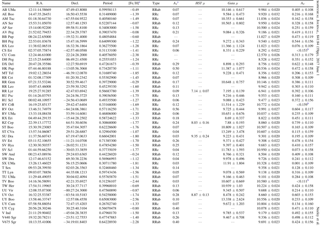
Table 6
Galactic RR Lyrae Sample
Name R.A. Decl. Period [Fe/H]a Type AV
a
HSTμ Gaiaμ μ AV
AB UMa 12:11:14.58669 47:49:43.8088 0.59958113 −0.49 RRab 0.07 L 10.146±0.617 9.984±0.020 0.405±0.108 AE Boo 14:47:35.26451 16:50:43.5538 0.31489000 −1.39 RRc 0.07 L 9.584±0.473 9.920±0.032 0.216±0.168 AM Tuc 01:18:30.64730 −67:55:04.9522 0.40580160 −1.49 RRc 0.07 L 10.353±0.661 11.036±0.024 0.162±0.158 AN Ser 15:53:31.05070 12:57:40.1293 0.52207144 −0.07 RRab 0.12 L 10.565±0.802 9.950±0.024 0.328±0.158
AP Ser 15:14:00.92200 09:58:51.8100 0.34083000 −1.58 RRc 0.13 L L 10.500±0.024 0.251±0.159
AV Peg 21:52:02.79453 22:34:29.3787 0.39037470 −0.08 RRc 0.21 L 9.084±0.326 9.186±0.021 0.419±0.111
BB Pup 08:24:22.65000 −19:32:31.4000 0.48054884 −0.60 RRab L L L 11.027±0.029 0.473±0.119
BH Peg 22:53:01.03678 15:47:16.5999 0.64099300 −1.22 RRab 0.24 L 9.272±0.343 9.540±0.023 0.544±0.156 BX Leo 11:38:02.06518 16:32:36.1864 0.36275500 −1.28 RRc 0.07 L 11.366±1.124 11.023±0.021 0.076±0.109 CS Eri 02:37:05.75874 −42:57:48.0588 0.31133100 −1.41 RRc 0.06 L 8.331±0.229 8.292±0.022 <0.153b
CU Com 12:24:46.61000 22:24:28.2000 0.40576050 −2.38 RRc L L L 12.570±0.026 0.313±0.179
DH Peg 22:15:25.64000 06:49:21.4500 0.25551053 −1.24 RRc L L L 8.528±0.022 0.351±0.152
DX Del 20:47:28.35586 12:27:50.6919 0.47261673 −0.39 RRab 0.29 L 8.898±0.293 8.756±0.022 0.622±0.148 HK Pup 07:44:46.80188 −13:05:56.3068 0.73420730 −1.11 RRab 0.50 L 11.387±1.077 10.536±0.024 0.472±0.158 MT Tel 19:02:12.28034 −46:39:12.0870 0.31689740 −1.85 RRc 0.12 L 9.228±0.471 8.356±0.022 0.206±0.153
RR Cet 01:32:08.17309 01:20:30.2342 0.55302900 −1.45 RRab 0.07 L L 8.966±0.020 0.308±0.109
RR Gem 07:21:33.53246 30:52:59.4617 0.39729000 −0.29 RRab 0.17 L 10.648±0.757 10.146±0.021 0.386±0.111
RR Leo 10:07:43.46008 23:59:30.3292 0.45239330 −1.60 RRab 0.11 L L 9.942±0.021 0.303±0.110
RR Lyr 19:25:27.91285 42:47:03.6942 0.56683780 −1.39 RRab 0.09 7.14±0.07 7.195±0.139 6.941±0.019 0.392±0.106 RU Psc 01:14:26.03793 24:24:56.3725 0.39036500 −1.75 RRc 0.13 L 9.216±0.446 9.553±0.021 0.160±0.111 RU Scl 00:02:48.10957 −24:56:43.0689 0.49335500 −1.27 RRab 0.06 L 9.088±0.423 9.477±0.023 0.372±0.156 RV CrB 16:19:25.85137 29:42:47.6404 0.33168000 −1.69 RRc 0.12 L 11.514±1.229 10.772±0.024 <0.159b RV Oct 13:46:31.74979 −84:24:06.3861 0.57116250 −1.71 RRab 0.56 L 9.725±0.444 9.991±0.027 0.604±0.117 RV UMa 13:33:18.08438 53:59:14.6081 0.46806000 −1.20 RRab 0.06 L 10.651±0.676 10.037±0.021 0.235±0.109 RX Eri 04:49:44.29135 −15:44:28.2502 0.58724622 −1.33 RRab 0.18 L 8.69±0.337 8.822±0.020 0.451±0.111 RZ Cep 22:39:13.17772 64:51:30.6036 0.30868000 −1.77 RRc 0.24 8.03±0.16 7.88±0.193 8.060±0.020 0.739±0.110 ST Boo 15:30:39.23085 35:47:04.3057 0.62228600 −1.76 RRab 0.07 L 10.809±1.027 10.507±0.021 0.165±0.109 ST CVn 13:57:34.06087 29:51:28.6887 0.32904500 −1.07 RRc 0.04 L 13.249±3.478 10.607±0.024 0.115±0.159 SU Dra 11:37:56.60743 67:19:47.0633 0.66042001 −1.80 RRab 0.03 9.35±0.24 9.223±0.431 9.301±0.020 0.195±0.109 SV Eri 03:11:52.10655 −11:21:14.0708 0.71385300 −1.70 RRab 0.26 L 9.371±0.427 9.308±0.022 0.478±0.154 SV Hya 12:30:30.50357 −26:02:51.1231 0.47854280 −1.50 RRab 0.25 L 9.397±0.401 9.683±0.023 0.410±0.157 SV Scl 01:44:59.66250 −30:03:33.3859 0.37735039 −1.77 RRc 0.04 L 11.783±1.593 10.950±0.024 0.073±0.158 SW And 00:23:43.08936 29:24:03.6365 0.44226020 −0.24 RRab 0.12 L 8.766±0.321 8.504±0.020 0.409±0.108 SW Dra 12:17:46.63152 69:30:38.2236 0.56966993 −1.12 RRab 0.04 L 9.978±0.496 9.726±0.021 0.241±0.112 SX UMa 13:26:13.46025 56:15:25.0606 0.30711780 −1.81 RRc 0.03 L 11.91±1.804 10.328±0.022 0.001±0.109
T Sex 09:53:28.39930 02:03:26.3563 0.32468460 −1.34 RRc 0.14 L L 9.358±0.021 0.128±0.110
TT Lyn 09:03:07.78856 44:35:08.1213 0.59743436 −1.56 RRab 0.05 L 9.078±0.569 9.138±0.020 0.316±0.109 TU UMa 11:29:48.49055 30:04:02.4094 0.55765870 −1.51 RRab 0.07 L 9.166±0.463 9.101±0.020 0.284±0.108 TV Boo 14:16:36.58091 42:21:35.6927 0.31256107 −2.44 RRc 0.03 L 10.607±0.669 10.580±0.021 <0.111b TW Her 17:54:31.19965 30:24:37.7117 0.39960010 −0.69 RRab 0.13 L 10.939±1.03 10.224±0.024 0.424±0.158 UU Vir 12:08:35.07300 −00:27:24.3000 0.47560890 −0.87 RRab 0.06 L 9.345±0.507 9.688±0.021 0.214±0.110 UV Oct 16:32:25.53387 −83:54:10.5183 0.54258000 −1.74 RRab 0.28 8.87±0.13 8.478±0.242 8.660±0.022 0.603±0.153 UY Boo 13:58:46.33747 12:57:06.4558 0.65083000 −2.56 RRab 0.10 L 13.338±2.624 10.556±0.020 0.233±0.109 UY Cam 07:58:58.88054 72:47:15.4203 0.26702740 −1.33 RRc 0.07 L 9.672±1.203 10.804±0.024 0.134±0.160
UY Cyg 20:56:28.30246 30:25:40.3104 0.56070478 −0.80 RRab 0.40 L L 10.078±0.021 0.471±0.110
V Ind 21:11:29.90402 −45:04:28.3835 0.47960170 −1.50 RRab 0.13 L 9.785±0.537 9.179±0.023 0.492±0.155 V440 Sgr 19:32:20.78211 −23:51:12.7553 0.47747883 −1.40 RRab 0.26 L 9.467±0.708 9.336±0.021 0.498±0.112
V675 Sgr 18:13:35.41006 −34:19:01.8403 0.64228930 −2.28 RRab 0.40 L L 9.691±0.023 0.424±0.156
8
The
Astrophysical
Journal,
841:84
(
19pp
)
,
2017
June
1
Neeley
et
Table 6
(Continued)
Name R.A. Decl. Period [Fe/H]a Type AV
a
HSTμ Gaiaμ μ AV
VX Her 16:30:40.79990 18:22:00.5524 0.45535984 −1.58 RRab 0.14 L 10.219±0.581 9.878±0.024 0.331±0.158 W Crt 11:26:29.64190 −17:54:51.6812 0.41201459 −0.54 RRab 0.12 L 10.207±0.664 10.815±0.028 0.168±0.119 WY Ant 10:16:04.97700 −29:43:42.9000 0.57434560 −1.48 RRab 0.18 L 10.41±0.598 10.067±0.021 0.402±0.110 X Ari 03:08:30.88520 10:26:45.2282 0.65117230 −2.43 RRab 0.56 L 8.468±0.239 8.660±0.020 0.704±0.108
XX And 01:17:27.41498 38:57:02.0359 0.72275700 −1.94 RRab 0.12 L L 10.253±0.020 0.308±0.109
XZ Cyg 19:32:29.30486 56:23:17.4900 0.46659934 −1.44 RRab 0.30 8.98±0.22 9.03±0.314 8.946±0.021 0.240±0.111 YZ Cap 21:19:32.41125 −15:07:01.1574 0.27345630 −1.06 RRc 0.20 L 11.358±1.188 10.325±0.022 0.296±0.113
Notes.
a
Adopted from Feast et al.(2008);AV =3.1E B( -V). b
Fit only provided upper limit for these stars.
9
The
Astrophysical
Journal,
841:84
(
19pp
)
,
2017
June
1
Neeley
et
and has recently been employed on classical Cepheids by Gieren et al.(2005)and Inno et al.(2016). The reddening law we adopted was that of Cardelli et al. (1989), which we extended into the IRAC and WISE bands according to Indebetouw et al.(2005)and Madore et al.(2013)respectively. The weights in the fit were determined by the sum in quadrature of the uncertainties in the apparent mean magni-tudes and predicted absolute magnimagni-tudes of the star, where the uncertainty of the predicted absolute magnitude is given by the dispersion of the PLZ relation of the corresponding wave-length. As a consequence, the IRAC bands have the most weight in determining the distance modulus, since the PLZ relations have the lowest dispersion at these wavelengths, and the IRAC mean magnitudes are more precise than those determined with WISEdata. The shorter wavelengths provide the leverage necessary tofit the extinction. The results of thisfit are given in the last two columns of Table 6.
To assess the ability of the theoretical PLZ relation to fit the distance moduli of all sample stars at different wavelengths, we have transformed all average magnitudes into semi-empirical absolute magnitudes using the best-fit distance moduli and extinctions from Table 6. The residuals between the calculated (from observed apparent magnitude) and predicted(from the PLZ relation)absolute magnitudes in each band are shown in Figure5. Individual stars are shown as small open circles, while the average residual in each band is over-plotted asfilled circles. The dashed lines represent the standard deviation around the mean of the average residuals. The IRAC,W1, andW2 bands offer the smallest dispersion. Predicted absolute magnitudes in the JHK bands tend to be brighter than the calculated absolute magnitude. There are three possibilities for this discrepancy:(1)the reddening law is inappropriate for these bands, (2) mean magnitudes calculated from JHKtemplates are systematically too faint,
or (3) the color temperature relations used to transform the bolometric light curves into the observational plane are incorrect for NIR wavelengths. The first point is unlikely, because the effect of reddening is low at NIR wavelengths, and the coefficients of the reddening law would have to change by as much as 50%. We see no systematic offset between mean magnitudes derived from JHK templates and observed light curves, but we note that less than half the stars in our sample have NIR light curves with high enough phase coverage to measure an accurate mean magnitude. Further observations are needed to see if this resolves the discrepancy with theory, or if the color temperature relations need some adjustment in theJHKbands.
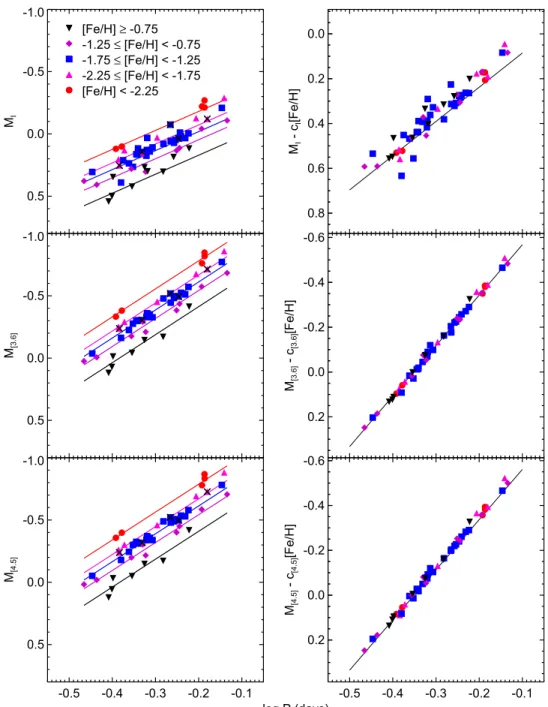
In Klein (2014), a multi-wavelength approach similar to ours was used to fit distances and extinctions of RRLs, but the effects of metallicity were ignored. In their Figure6.20, PL relations from optical to MIR are shown with remarkably small scatter. However the scatter is by design artificially small, since the optimal solution is estimated by minimizing the residuals of the different bands. Our synthetic PLZ relations provide a method to estimate the effect of metallicity on the determination of distances. The left panels of Figure 6 show how the RRLs in our sample lie in the period–magnitude plane when metallicity is ignored. Stars were divided intofive metallicity bins, and the predicted PL relation for the median of each bin is shown as the solid line in the corresponding color. The dispersion around individual relations is quite low(with much of it still due to a spread in metallicity), but if we consider all RRLs covering a large range of metallicity as a single population, the dispersion around the average metallicity is large(0.12, 0.13, and 0.13 in the I, [3.6], and [4.5] bands respectively). In the right panels of Figure6, the metallicity term has been subtracted out, and the vertical axis is now Ml-cl[Fe H]. Now the
dispersion around the theoretical relation is almost an order of magnitude smaller (0.053, 0.019, and 0.017 mag in the I, Figure 3.SampleWISEand IRAC light curves for the Galactic RRL star SU Dra. TheW1,[3.6]andW3 bands are offset by±1 mag for better visibility. The smoothed light curve generated by GLOESS is shown as the red line.
10
[3.6], and [4.5] bands respectively). These panels illustrate the drastic improvement one can expect in the accuracy of distance determinations when accounting for metallicity. Assuming the theoretical PLZ relations correctly characterize the effect on the zero point due to metallicity, using PLZ
relations over PL relations will reduce the uncertainty of distance measurements from 13% to 2%. A similar argument can be shown using PWZ relations (Figure 7). Here, the dispersion in the PW relation once metallicity has been removed is even smaller (0.012 mag for I-IRAC PWZ Table 7
Updated Photometry for RR Lyrae in M4
Name Period [3.6] [4.5] [5.8] [8.0]
V01 0.28888261 11.304±0.023 11.278±0.073 L L
V02 0.5356819 11.002±0.093 10.949±0.031 L 10.863±0.139
V03 0.50667787 L 11.015±0.026 L 10.941±0.135
V05 0.62240112 10.833±0.036 10.803±0.029 10.774±0.125 10.711±0.077
V06 0.3205151 11.226±0.044 L 11.183±0.053 L
V07 0.49878722 11.039±0.043 11.026±0.032 11.041±0.156 L
V08 0.50822359 10.964±0.045 10.945±0.027 10.904±0.226 10.84±0.141
V09 0.57189447 10.891±0.043 10.867±0.039 10.778±0.142 10.721±0.142
V10 0.49071753 11.063±0.048 11.053±0.032 10.997±0.16 11.005±0.16
V11 0.49320868 L 11.069±0.03 L 10.931±0.13
V12 0.4461098 11.169±0.064 11.146±0.034 11.211±0.171 11.175±0.171
V14 0.46353111 11.159±0.061 11.128±0.039 11.075±0.169 11.054±0.169
V15 0.44366077 11.186±0.044 L 11.029±0.158 L
V16 0.54254824 10.899±0.036 10.884±0.027 10.744±0.122 10.743±0.122
V18 0.47879201 10.999±0.051 10.941±0.05 10.804±0.13 10.812±0.13
V19 0.46781108 11.121±0.045 L 11.119±0.136 L
V20 0.30941948 10.972±0.105 10.943±0.106 10.935±0.077 11.066±0.039
V21 0.47200742 10.772±0.056 10.771±0.05 10.569±0.123 10.556±0.123
V22 0.60306358 10.815±0.047 10.792±0.028 10.744±0.092 10.702±0.092
V23 0.29861557 11.073±0.034 11.088±0.021 10.991±0.045 10.987±0.053
V24 0.54678333 10.946±0.042 10.946±0.027 10.798±0.11 10.853±0.11
V25 0.61273479 10.83±0.046 10.789±0.031 10.706±0.139 10.689±0.139
V26 0.54121739 10.959±0.045 10.928±0.037 10.757±0.165 10.79±0.165
V27 0.61201829 10.84±0.041 L 10.952±0.121 L
V28 0.52234107 10.997±0.04 10.981±0.038 11.014±0.178 11.026±0.178
V29 0.52248466 11.002±0.044 L L L
V30 0.26974906 L L L L
V31 0.50520423 L L L L
V32 0.57910475 L L L L
V33 0.61483542 L L L L
V34 0.5548 L L L L
V35 0.62702374 L L L L
V36 0.54130918 L 10.939±0.038 L 10.864±0.142
V37 0.24734353 11.428±0.043 11.422±0.02 11.384±0.026 11.402±0.03
V38 0.57784635 10.772±0.047 10.751±0.033 10.757±0.104 10.77±0.104
V39 0.623954 10.841±0.041 10.821±0.025 10.757±0.091 10.794±0.091
V40 0.38533005 10.893±0.051 10.865±0.034 10.708±0.153 10.842±0.366
V41 0.2517418 11.469±0.036 11.457±0.019 11.447±0.038 11.452±0.038
V42 0.3068549 11.298±0.11 L L L
V49 0.22754331 11.492±0.035 11.495±0.029 11.4±0.029 11.397±0.029
V52 0.85549784 10.511±0.041 10.473±0.034 10.378±0.071 10.383±0.01
V61 0.26528645 11.452±0.053 11.414±0.018 11.337±0.03 11.328±0.031
C01 0.2862573 11.266±0.102 11.224±0.11 11.122±0.112 10.7±0.235
Table 8
Calibrated Empirical PL Relations for M4
Band aa ba σb aa ba σb aa ba σb
FO FU FU+FO
[3.6] −1.008±0.170 −2.75±0.42 0.075 −1.155±0.089 −2.34±0.14 0.040 −1.112±0.089 −2.30±0.11 0.055
[4.5] −1.032±0.170 −3.00±0.33 0.056 −1.170±0.089 −2.36±0.17 0.044 −1.139±0.089 −2.34±0.10 0.053
[5.8] −1.220±0.29 −3.18±0.56 0.10 −1.239±0.11 −2.43±0.34 0.096 −1.190±0.09 −2.34±0.20 0.10
[8.0] −1.263±0.55 −3.13±1.20 0.20 −1.270±0.10 −2.45±0.28 0.074 −1.187±0.10 −2.22±0.25 0.12
Notes. a
m=a+blog .P b
Dispersion of RRLs in the cluster M4.
11
relations). This could be because PWZ relations are red-dening free (they depend only on the reddening law, not the extinction of individual objects), or because the PWZ relations include a color term and reduce the scatter because they take into account the width in temperature of the instability strip.
5.1. Comparison with the HST
Prior to theGaiarelease, the only geometric measurement of RRL distances was the parallax offive stars(RR Lyr, RZ Cep, SU Dra, UV Oct, and XZ Cyg)measured using theHSTFGS (Benedict et al.2011). With onlyfive calibrators available, the precision of the absolute zero point of RRL PL relations has Figure 4.Period dependence(bλ)for differentfilters. The predicted coefficients of PLZ relations from Marconi et al.(2015)and Table3of this work are shown as black circles. Empirical measurements from the literature are shown for comparison according to the legend.
Figure 5.Residual between the absolute magnitude using the best-fit distance moduli and extinctions and the predicted absolute magnitude from theoretical PLZ relations for all galactic RRLs in each band. Individual stars are shown with open circles, and the average residual for each band is shown as afilled circle. The error bars represent the standard deviation in the residuals of the individual stars. The solid line is the weighted mean of the average residuals, and the dashed lines are 1σfrom the mean. Note that because this is a weightedfit, the solid line passes the points with the most weight([3.6]and[4.5])and not through zero.
12
been severely limited. In this section, we compare the HST parallaxes with results based on the theoretical PLZ relations.
Table6presents the distance moduli and extinctions derived in Benedict et al.(2011), compared with the values estimated in this work. The distance moduli comparison is also shown in Figure 8. Two stars, RR Lyr and UV Oct, exhibit a 2.7 and 1.6σ tension, respectively, between our method and the HST distance moduli. Three stars(RR Lyr, SU Dra, and UV Oct)are alsofit with a significantly larger extinction using our method. The extinctions adopted in Benedict et al.(2011)are from Feast et al.(2008), where stars werefit using 3D Galactic extinction models while assuming a distance based on MV -[Fe H]or
preliminary PL(K)relations. Figure 9 compares the residuals with predicted absolute magnitude when correcting observa-tions using theHSTparallaxes and extinctions(left panel)as a
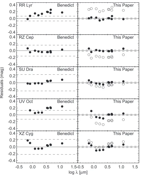
function of wavelength. The residuals of four stars (RR Lyr, RZ Cep, SU Dra, and UV Oct)present a trend with wavelength when using the HST derived parameters, indicating the extinction assumed for these stars in Benedict et al. (2011) is incorrect. The vertical offset seen in RR Lyr and UV Oct is a consequence of the difference in distance modulus we measure. In contrast, the right panel shows no offsets or trends, suggesting good agreement with theory across all wavelengths. Clearly, the observations and theory are at odds for some of these stars. The discrepancy with predicted absolute magnitude shows no trend with period, distance, or metallicity, which indicates the problem may lie with individual parallax and extinction measurements. We should note that both RR Lyr and UV Oct exhibit the Blazhko effect, and it is possible that this is affecting the mean magnitude of these stars. However, XZ Cyg Figure 6.Calculated absolute magnitude vs. period offield RRL stars for theI, 3.6, and 4.5μm bands. Left panels: the stars have been separated into metallicity bins from low(black triangles)to high(red circles)metal abundance. Predicted relations for the median of each metallicity bin are shown with solid lines. Right panels: the metallicity term(cλ∗[Fe/H])has been subtracted from the vertical axis(normalized to solar metallicity,[Fe/H]=0.0 dex.
13
Figure 7.Period–Wesenheit–metallicity relation offield RRL stars. Predicted relations for thefive metallicity bins are shown with solid lines. In the right panel the metallicity term has been subtracted from the vertical axis.
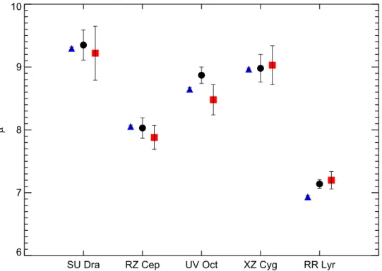
Figure 8.A direct comparison of the distance modulus offive stars obtained with three methods:(1)the method presented in this paper(blue triangles),(2)HST
parallax measurements from Benedict et al.(2011) (black circles), and(3)proper motion parallaxes from the Tycho–Gaiaastrometric solution(TGAS) (red squares). For both theHSTand TGAS distance moduli, the error bars are dominated by the error in the parallax.
14
is also a Blazhko star, and all methods are in good agreement for this star.
5.2. Comparison with Gaia DR1
We can also compare the distance moduli obtained above with the recent parallax measurements from theGaiamission. Gaia’s first data release (DR1) became public on 2016 September 14 (Gaia Collaboration et al. 2016, 2016). This release included proper motion parallax measurements for stars in common with the Tycho-2 catalog, and are based on the Tycho–Gaia astrometric solution (TGAS, Michalik et al.
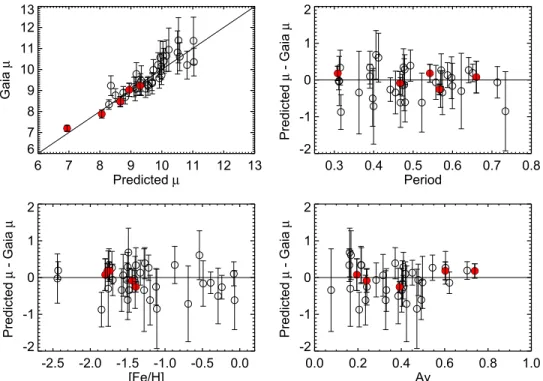
2015). TGAS parallaxes were available for 41 of the stars in our sample, with uncertainties ranging from σπ/π=0.06 to σπ/π=0.83. The distance moduli from TGAS parallaxes are given in Table6. In Figure10we compare the TGAS results with the distance moduli obtained in this paper for stars with
<55% uncertainty in the TGAS parallax. The top right panel is a one-to-one comparison between the two methods. The five stars with previously determined HST parallaxes are high-lighted with filled red circles. For the majority of stars, the methods agree within 1σ. Only four stars (AM Tuc, RR Lyr, MT Tel, V Ind) are outliers, and all are within 2σ. Both the dispersion and individual uncertainty increase with distance. The dispersion is 0.30 for stars withμ0<9.5 and 0.46 for stars with μ0>9.5, and the average uncertainty in the TGAS distance is twice as large for stars with μ0>9.5 mag. The remaining panels in Figure10 show the residual between the two methods as a function of stellar parameters, indicating there are no trends with period, metallicity, or AV. This
confirms that the residual error between our best-fit value and the TGAS parallax are likely due to the statistical uncertainties in the TGAS results.
Figure 9.Comparison of the offset with predicted absolute magnitude when using theHST-derived distance modulus and extinction from Benedict et al.(2011) (left panels)and in this paper(right panels)as a function of wavelength. The dashed lines indicate the uncertainty in the distance moduli. The right panels also include as open circles the residual when using the TGAS distances and the extinction from this paper. Trends with wavelength indicate the extinction is inconsistent with theoretical predictions, while on overall offset suggests the distance is inconsistent with theory.
15
6. M4 Distance
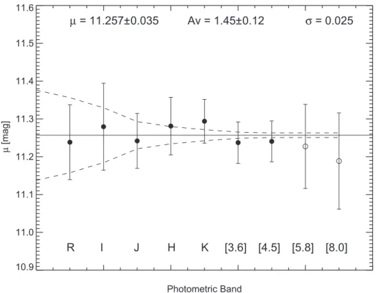
We can use globular clusters as an additional laboratory to test the theoretical PLZ relations. Globular clusters offer the advantage that there are many RRLs at roughly the same distance, reddening, and metallicity. For the closest globular cluster to us, M4(NGC 6121), if we assume a 10 pc radius the expected difference in distance modulus between stars in the front and back of the cluster is about 0.02 mag. Since this is smaller than the expected dispersion in the PLZ relation, we cannot accurately measure the distances and extinctions for individual stars. However, we can measure the average distance and extinction for the cluster as a whole.
The distance modulus and reddening to M4 was fit in a similar method to the Galactic RRLs, but instead offitting an individual distance and extinction for each star, we derived the averageμ0andAV. A reddened distance modulus for each
band was calculated by averaging the difference between observations and predicted absolute magnitude from the theoretical PLZ relations. The true distance modulus and visual extinction were then fit using a least-squares fit as in Equation (1), but now the reddening coefficients Aλ/AV are
defined by a reddening law specific to M4 (Hendricks et al.
2012). This reddening law accounts for the fact that the cluster is behind theρOph cloud by adopting a higher dust parameter (RV = 3.62) than the Cardelli law (RV = 3.1).
Figure11shows the extinction-corrected distance moduli for each band. Single epoch archival data for the two longer Spitzerbands are also shown for reference as open circles, but were not included in the fit. The dashed lines represent how the uncertainty in extinction propagates with wavelength. The final distance modulus is μ0=11.257±0.035, and the V-band extinction is AV=1.45±0.12. This is consistent with our results from purely empirical NIR and MIR PL
relations,μ0=11.283±0.010±0.018(Braga et al.2015), μ0=11.353±0.095 at 3.6μm andμ0=11.363±0.095 at 4.5μm (Section 4) respectively. Our measured distance modulus of μ0=11.257 is also consistent with recent measurements from a variety of other primary distance methods, and we will highlight a few here(see Section2 of Braga et al.2015for a more complete discussion). Hendricks et al. (2012) estimate AV=1.39±0.01 and μ0=11.28± 0.06 so our measurements are within 1σ. The distance to M4 has also recently been measured by Kaluzny et al. (2013)
using three eclipsing binary stars. They obtained μ0=11.30±0.05, which is also in agreement with our method.
Figure 12 shows the MIR observations transformed into absolute magnitude with the best-fit distance modulus and extinction. Fundamental pulsators(RRab)are shown withfilled red circles while FO pulsators(RRc)are shown as open blue circles. In the right panels, the period of the RRc variables have been fundamentalized. The theoretical PL relation for the metallicity of the cluster([Fe/H]=−1.1)is over-plotted. The bottom two panels show the first PL relations at the 5.8 and 8.0μm bands. Since only single epoch observations are available for these two bands, the dispersion is larger than the anticipated intrinsic scatter of the PL relation. The data lie slightly above the theoretical line but, as expected, the longer wavelengths have lower angular resolution and are much more susceptible to blending. Overall, the theoretical slope fits the data well in all four IRAC bands.
7. Discussion and Conclusion
We have presented the first theoretical PLZ relations for RRLs at MIR wavelengths. The relations were constructed from a large grid of nonlinear, time-dependent convective Figure 10.Top left: one-to-one comparison of the distance moduli derived in this paper and determined from thefirst release of TGAS parallaxes. Thefive stars with previously determinedHSTparallaxes are highlighted with closed red circles. Given that all but two stars agree within 1σ, this may indicate that the TGAS errors are overestimated as suggested in Casertano et al.(2016)and Gould et al.(2016). Top right: residuals between predicted and TGAS parallaxes as a function of the pulsation period. Bottom left: residuals between predicted and TGAS parallaxes as a function of the metal abundance. Bottom right: residuals between predicted and TGAS parallaxes as a function of thefitted visual band extinction.
16
hydrodynamical models over a large range of metal abundances and fixed helium enrichment. We have shown that metallicity plays an important role in the zero point of these relations, and increasing the metal content decreases the zero point (i.e., RRLs with higher metal abundances are fainter). With this in mind, we investigated the effect this would have on the RRLs in the CRRP sample, and found that, if ignored, the metallicity spread(−2.6<[Fe/H]<−0.1)results in a scatter of 0.13 mag. When the metallicity component is accounted for, the scatter is reduced to 0.02 mag. Clearly, metallicity must be considered when analyzing a multi-metallicity sample. Consider the error budget for the Carnegie–Chicago Hubble Program, as outlined in Beaton et al. (2016). In order to obtain the projected 3% measurement of H0, it is necessary to keep the precision of
distances measured via the RRL PL relation <1.7%. They estimated the impact of a multiple metallicity sample using the scatter in theH-band PL relation in the globular clusterωCen. Their estimate(σastro=0.06 mag)is half the scatter we observe in the CRRP Galactic RRL sample(although we note thatωCen covers a different range in [Fe/H] than the CRRP sample). Propagating our larger value ofσastro=0.13 mag corresponds to a 3% error on distances, too large for our desired uncertainty in H0. To reduce the uncertainty, we must empirically calibrate the
metallicity component. CRRP offers this opportunity. The globular clusters in the CRRP sample offer the necessary statistics to nail down the period dependence of the RRL PL relation, and test for any metallicity dependence of such a period slope. Once the period dependence isfixed, the Galactic RRLs, for which we will have milliarcsecond parallax measurements from futureGaiareleases, will be used to calibrate the zero point and metallicity dependence. Furthermore, we will utilize multi-wavelength data in order to fit the extinction of individual objects. It is important to note that since the metallicity
coefficient of the PLZ relation is wavelength independent, multi-wavelength data cannot be used to constrain the metallicity as well as the distance of individual RRLs. Instead we must have a prior measurement of[Fe/H]with a maximum uncertainty of ±0.1 dex in order to measure the distance of a single RRL to 2% precision. Currently, the metallicity measurements available in the literature are very inhomogeneous. They are measured through a variety of methods and placed on different scales, and achieving our required accuracy is unlikely. Therefore, we have undertaken a program to provide homogenous measurements of [Fe/H]from high-resolution spectra for all of the RRLs in our sample.
We also present a method to fit the distance modulus and extinction of individual RRLs by comparing multi-wavelength observations to our theoretical PLZ relations. At this point the error bars on the TGAS distances are too large to make any meaningful comparison with our results for the full CRRP sample. We can however directly compare our distances to those obtained by Benedict et al.(2011)with theHSTforfive stars. We find that there is >1σ disagreement between the theoretical and observational results for two of the five stars, UV Oct and RR Lyr. For these two stars, we see both an offset and a trend with wavelength in the residuals between observations and theory. The trend with wavelength when using the Benedict et al.(2011)parallaxes suggests an incorrect value for extinction, but even when this is corrected for, the offset persists. We offer two possible explanations for this offset. The first possibility is that the parallax determined in Benedict et al.(2011)is incorrect for these two stars. Wefind it unlikely that some unknown systematics are affecting the parallax measurement of individual stars, but note that the Benedict et al.(2011)parallax measurement for UV Oct is in greater than 1σdisagreement with the TGAS distance, and that Figure 11.Derived extinction-corrected distance modulus of M4 for all available bands. Only points plotted withfilled circles were used in calculating the band-averaged distance modulus and extinction, and the remaining bands are shown only for reference. The solid line is the average distance modulus, and the dashed lines indicate how the uncertainty in extinction propagates with wavelength.
17
there are typographical errors in both the parallax published for RZ Cep.21 The second possibility is that the MIR photometry for RR Lyr and UV Oct is inconsistent with the average behavior of these stars. Both of these stars are Blazhko variables and exhibit long-term amplitude modulations in their optical light curves. Since theSpitzerphotometry was collected over a single pulsation phase, the average magnitude derived from one cycle may be different than one derived over many cycles. However, the WISE photometry is randomly sampled over many different pulsation cycles, and we do not see any significant offset between the Spitzer and WISE mean
magnitudes. Additionally, XZ Cyg is also a Blazhko star and shows no offset between the distance derived from theory and by parallax measurement.
Our synthetic PLZ relations agree well with empirical PL and PLZ relations measured both in Galactic globular clusters and in halo RRLs. These relations demonstrate the potential of RRLs to be high-precision distance indicators, particularly at MIR wavelengths where the effects of extinction and intrinsic dispersion (after removing the metallicity dependence) are smallest. We alsofit multi-wavelength observations of RRLs in the Galacticfield and in M4 to the theoretical PLZ relations to provide new distance and extinction estimates. The distance moduli of the Galactic RRLs are consistent with preliminary parallax measurements from theGaiamission. In M4, wefit an averaged distance modulus and extinction for the cluster, resulting in μ0=11.257±0.035 and AV=1.45±0.12. Figure 12.MIR photometry of M4 RRL corrected to absolute magnitude using best-fit distance and extinction. RRc stars are shown with open blue circles and RRab stars withfilled red circles. The theoretical PL relations for the cluster’s metallicity is shown as the black lines. As in Figure2, the left panels show separate relations for the RRc and RRab stars and in the right panels the RRc stars have been fundamentalized.
21
Two different values for the parallax of RZ Cep are reported in the text and Table8 of Benedict et al. (2011). We use the value found in the text,
πabs=2.54±0.19 mas, which is consistent with the distance modulus reported in their Table8, and is more consistent with our PLZ relations.
18
Both of these values are consistent with estimates from a variety of other methods, further implying the validity of the theoretical PLZ relations.
We thank the anonymous referee for helpful comments that improved the applicability of this manuscript.
This work has made use of data from the European Space Agency (ESA) mission Gaia (https://www.cosmos.esa.int/ gaia), processed by the Gaia Data Processing and Analysis Consortium (DPAC, https://www.cosmos.esa.int/web/gaia/ dpac/consortium). Funding for the DPAC has been provided by national institutions, in particular the institutions participat-ing in theGaiaMultilateral Agreement.
This work is based in part on archival data obtained with the Spitzer Space Telescope, which is operated by the Jet Propulsion Laboratory, California Institute of Technology under a contract with NASA. Support for this work was provided by an award issued by JPL/Caltech.
This publication makes use of data products from the Wide-field Infrared Survey Explorer, which is a joint project of the University of California, Los Angeles, and the Jet Propulsion Laboratory/California Institute of Technology, funded by the National Aeronautics and Space Administration. This publica-tion makes use of data products from the Two Micron All Sky Survey, which is a joint project of the University of Massachusetts and the Infrared Processing and Analysis Center/California Institute of Technology, funded by the National Aeronautics and Space Administration and the National Science Foundation.
Facilities: Spitzer (IRAC),WISE,Gaia.
References
Beaton, R. L., Freedman, W. L., Madore, B. F., et al. 2016,ApJ,832, 210
Benedict, G. F., McArthur, B. E., Feast, M. W., et al. 2011,AJ,142, 187
Bono, G. 2003, ASPC,298, 245
Bono, G., Braga, V. F., Pietrinferni, A., et al. 2016, MmSAI,87, 358
Bono, G., Caputo, F., Castellani, V., et al. 2003,MNRAS,344, 1097
Bono, G., Caputo, F., Castellani, V., & Marconi, M. 1999,ApJ,512, 711
Bono, G., Caputo, F., Castellani, V., Marconi, M., & Storm, J. 2001,MNRAS,
326, 1183
Braga, V. F., Dall’Ora, M., Bono, G., et al. 2015,ApJ,799, 165
Brott, I., & Hauschildt, P. H. 2005, in The Three-Dimensional Universe with Gaia, ed. C. Turon, K. S. O'Flaherty, & M. A. C. Perryman(ESA SP-576; Noordwijk: ESA),565
Cáceres, C., & Catelan, M. 2008,ApJS,179, 242
Caputo, F., Castellani, V., Marconi, M., & Ripepi, V. 2000,MNRAS,316, 819
Cardelli, J. A., Clayton, G. C., & Mathis, J. S. 1989,ApJ,345, 245
Carey, S., Ingalls, J., Hora, J., et al. 2012,Proc. SPIE,8442, 84421Z
Casertano, S., Riess, A. G., Bucciarelli, B., & Lattanzi, M. G. 2016, arXiv:1609.05175
Castelli, F., & Kurucz, R. L. 2004, arXiv:astro-ph/0405087
Catelan, M., Pritzl, B. J., & Smith, H. A. 2004,ApJS,154, 633
Coppola, G., Marconi, M., Stetson, P. B., et al. 2015,ApJ,814, 71
Dall’Ora, M., Storm, J., Bono, G., et al. 2004,ApJ,610, 269
Dambis, A. K., Rastorguev, A. S., & Zabolotskikh, M. V. 2014,MNRAS,
439, 3765
Dékány, I., Minniti, D., Catelan, M., et al. 2013,ApJL,776, L19
Fazio, G. G., Hora, J. L., Allen, L. E., et al. 2004,ApJS,154, 10
Feast, M. W., Laney, C. D., Kinman, T. D., van Leeuwen, F., & Whitelock, P. A. 2008,MNRAS,386, 2115
Freedman, W., Scowcroft, V., Madore, B., et al. 2012, The Carnegie RR Lyrae Program, Spitzer Proposal,90002
Freedman, W. L., Grieve, G. R., & Madore, B. F. 1985,ApJS,59, 311
Freedman, W. L., Wilson, C. D., & Madore, B. F. 1991,ApJ,372, 455
Gaia Collaboration, Brown, A. G. A., Vallenari, A., et al. 2016,A&A,595, A2
Gieren, W., Pietrzyński, G., Soszyński, I., et al. 2005,ApJ,628, 695
Gould, A., Kollmeier, J. A., & Sesar, B. 2016, arXiv:1609.06315
Grevesse, N., & Noels, A. 1993, in Origins and Evolution of the Elements, ed. N. Pratzo, E. Vangioni-Flam, & M. Casse(Heidelberg: ARI),15
Grevesse, N., & Sauval, A. J. 1998,SSRv,85, 161
Hendricks, B., Stetson, P. B., VandenBerg, D. A., & Dall’Ora, M. 2012,AJ,
144, 25
Indebetouw, R., Mathis, J. S., Babler, B. L., et al. 2005,ApJ,619, 931
Inno, L., Bono, G., Matsunaga, N., et al. 2016,ApJ,832, 176
Jameson, R. F. 1986,VA,29, 17
Johnston, K., Scowcroft, V., Madore, B., et al. 2013, Spitzer Merger History and Shape of the Halo, Spitzer Proposal,10015
Kaluzny, J., Thompson, I. B., Rozyczka, M., & Krzeminski, W. 2013, AcA,
63, 181
Klein, C. R. 2014, PhD dissertation Univ. California, Berkeley
Klein, C. R., Richards, J. W., Butler, N. R., & Bloom, J. S. 2011,ApJ,738, 185
Longmore, A. J., Fernley, J. A., & Jameson, R. F. 1986,MNRAS,220, 279
Madore, B. F., & Freedman, W. L. 2012,ApJ,744, 132
Madore, B. F., Hoffman, D., Freedman, W. L., et al. 2013,ApJ,776, 135
Marconi, M., Bono, G., Caputo, F., et al. 2011,ApJ,738, 111
Marconi, M., Coppola, G., Bono, G., et al. 2015,ApJ,808, 50
Michalik, D., Lindegren, L., & Hobbs, D. 2015,A&A,574, A115
Monson, A. J., Beaton, R. L., Scowcroft, V., et al. 2017,AJ,153, 96
Neeley, J. R., Marengo, M., Bono, G., et al. 2015,ApJ,808, 11
Nishiyama, S., Tamura, M., Hatano, H., et al. 2009,ApJ,696, 1407
Pietrinferni, A., Cassisi, S., Salaris, M., & Castelli, F. 2006,ApJ,642, 797
Pietrukowicz, P., Kozłowski, S., Skowron, J., et al. 2015,ApJ,811, 113
Gaia Collaboration, Prusti, T., de Bruijne, J. H. J., et al. 2016,A&A,595, A1
Stetson, P. B. 1987,PASP,99, 191
Stetson, P. B. 1992, in ASP Conf. Ser. 25, Astronomical Data Analysis Software and Systems I, ed. D. M. Worrall, C. Biemesderfer, & J. Barnes (San Francisco, CA: ASP),297
![Figure 1. Top: difference in [4.5] magnitudes as a function of the effective temperature for a set of FU models computed at fixed stellar mass (0.716 M e ), luminosity ( log L L = 1.72 ), and chemical composition (Z=0.0003, Y=0.245)](https://thumb-us.123doks.com/thumbv2/123dok_es/3749597.643838/3.918.189.731.75.426/difference-magnitudes-function-effective-temperature-computed-luminosity-composition.webp)
![Figure 3. Sample WISE and IRAC light curves for the Galactic RRL star SU Dra. The W1, [3.6] and W3 bands are offset by ±1 mag for better visibility](https://thumb-us.123doks.com/thumbv2/123dok_es/3749597.643838/10.918.188.735.76.464/figure-sample-wise-curves-galactic-offset-better-visibility.webp)