Minimal distance from a point to n lines

Texto completo

(1)Vol. XX, No 2, Diciembre (2012) Matemáticas: 35–44. Matemáticas: Enseñanza Universitaria c Escuela Regional de Matemáticas Universidad del Valle - Colombia. Minimal distance from a point to n lines Martı́n E. Acosta. Carolina Mejı́a. Universidad Industrial de Santander. Universidad Nacional de Colombia. Carlos W. Rodrı́guez Universidad Industrial de Santander Received Aug. 15, 2012. Accepted Nov. 20, 2012. Resumen We present a solution to the problem of computing a point in the plane minimizing the distance to n given lines. We used an experimental mathematics approach: using dynamic geometry software, we gathered data which allowed us to conjecture and testing our hypothesis. Finally we formalized our reasoning to prove the conjecture. Although this solution was known, our method could be of interest. Palabras y frases claves: Minimal distance, experimental mathematics. Clasificación de la AMS: 51K99. 1. Introduction. In this work we describe an experimental mathematics strategy (see [1] ) to solve a geometric problem : we use dynamic geometry software to gather data, state and check conjectures, and then look for formal proofs of the conjectures that survives the experimental phase. We use the software CABRI II plus, which allows us to represent the problem and perform calculations. The dragging mode, characteristic of dynamic geometry software (see [2]), allows us to check our conjectures in a huge number cases. Although our solution is not new (see [5]), this experimental strategy could be of interest in research and mathematical education. The problem solved is the following: Problem 1 (MIN). Given n lines, determine a point minimizing the sum of the distances from this point to the n given lines. From now on we will use the symbol M IN to denote the above problem. Organization of the work. The paper is organized into two sections. Section one deals with the experimental work and the search for a suitable conjecture encompassing the experimental results. In section two we propose a conjecture and we prove it..

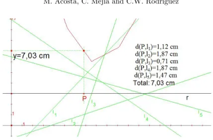
(2) 36. M. Acosta, C. Mejı́a and C.W. Rodrı́guez. Figure 1: First exploration.. 2. The problem and the experimental exploration. In this section we describe the experimental work carried out with CABRI II plus. We asked us: Which is the structure of the solution set of a typical instance of the problem M IN ? Initially, we considered configurations constituted by five lines, that is: we considered instances of the problem M IN , determined by no more than five lines. We used CABRI II plus to find the solution set of the instances considered, we looked for regularities arising in the computed solution sets, and then we used this information to formulate corresponding conjectures. Once a conjecture was proposed, we checked its soundness using new instances of the basic problem. Experimental work (with 5 lines) In the experimental work we planed to move a point around the plane and calculate the sum of its distances to the given lines in order to find some properties which could lead us to a conjecture. In the following experimental device, we put a point on a line, so we can drag the point on the line to reach all positions on it, and drag the line to reach all positions on the plane, and with the locus tool we represent the function of the sum of the distances to the given lines. 1. We drew a horizontal line r with a point P on it. Then, we dragged the point along the line, getting in this way all possible abscissas. After that we began to move the line itself, without changing its direction, getting in this way all the possible ordinates. 2. We measured the distances from P to the five given lines, we added those distances, and transferred this sum to the y axis (see Figure 1)..

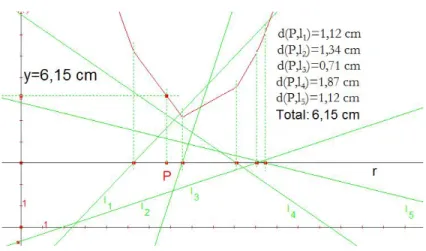
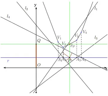
(3) Minimal distance from a point to n lines.. 37. Figure 2: Second exploration.. 3. We constructed a point Q whose abscissa is the abscissa of P and whose ordinate is the sum of the distances from P to the five given lines. 4. We drew the locus of Q with respect to P , and we obtained a polygonal line with a finite number of vertices, the abscissas of those vertices matched the abscissas of the intersection points of the horizontal line and the five given lines (see Figure 2). 5. We observed that one of those vertices had minimal ordinate. 6. We activated the trace of the locus, dragged the horizontal line, and we saw that there was one point for which the sum of distances to the five given lines was minimal (see Figure 3). Then, we observed that the point minimizing the distance belonged to the intersection of pairs of the five given lines. 7. We repeated the process many times, that is: we consider many configurations of lines and we used CABRI II plus to compute the solution-sets of each one of the configurations considered (see Figure 4). We observed that, for each one of the experiments performed, there was one point in the computed solution-set that belonged to the intersection of the five given lines.. 3. A succesful conjecture and its proof. Our conjecture is that at least one point of the solution-set belongs to the intersection of the given lines..

(4) 38. M. Acosta, C. Mejı́a and C.W. Rodrı́guez. Figure 3: Third exploration.. Figure 4: Fourth exploration..

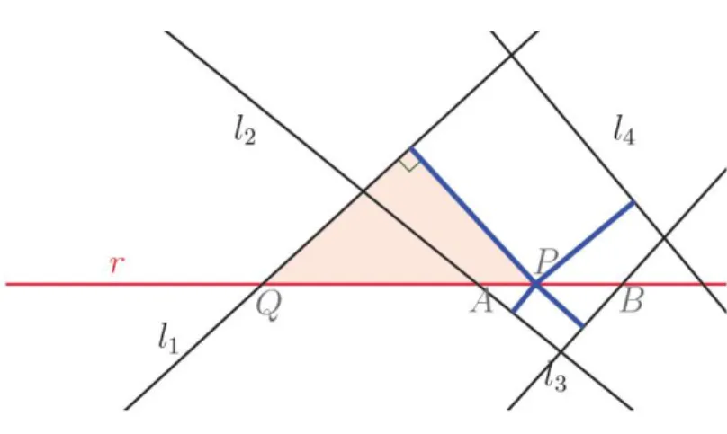
(5) Minimal distance from a point to n lines.. 39. Figure 5: Perpendiculars from P to the given lines.. Proposition 1. Suppose we have n given lines in the plane and suppose that they are not pairwise parallel.1 Given P, a point in the plane, we use the symbol Sp to denote the sum of the distances from P to the n given lines. Then, we have that Sp reaches its minimum value at one of the points located on the intersection of at least two of the n given lines. From now on, we use the term intersection points to denote the points that belong to the intersection of at least two of the given lines. Before proving the above proposition we have to prove next lemma. Lemma 1. Let r be a line, and suppose that r meets at least one of the n given lines, suppose that AB is a segment that is located between two consecutive intersection points of r with the n given lines2 , then the restriction of SP to AB is a linear function. Proof. We pick a point P on AB, and from P we draw perpendicular segments to the n lines, whose lengths are equal to the distances from P to the given lines (see Figure 5). If the lines are not parallel to r, each of those orthogonal segments is a cathetus of a right triangle with hypotenuse in r, being the other cathetus a segment of the corresponding line3 (see Figure 6). Clearly, when P moves to P 0 on AB, each of the right triangles defined by P is similar to the corresponding one defined by P 0 . We will prove inductively that the sum of distances from P to the given lines changes proportionally when P moves on the segment AB. Proof by induction Let us take initially two lines l1 and l2 . Let A, B be the intersection points of r with l1 and l2 , respectively. Let AD and BE be 1. If all lines are parallel, there is an infinity of points minimizing the distance to the lines. This case will be discussed in another paper. 2 If r cuts exactly one line, the segment becomes a point and the graph of SP becomes also a point. 3 If the lines are parallel to r they do not form triangles, but their distances to P will be constants and these constants will not affect the sum..

(6) 40. M. Acosta, C. Mejı́a and C.W. Rodrı́guez. Figure 6: Right triangle with hypotenuse in r.. the orthogonal segments to l1 and l2 , that arise from A and B (respectively)(see Figure 7). Note that SA is the length of AD and SB is the length of BE. Let P Q and P R be the orthogonal segments to l1 and l2 that arise from P . Now, given that 4ADB and 4P RB are similar, we have SA PR = . AB PB. Figure 7: Initial two lines, l1 and l2 .. 4BEA and 4P QA are similar too, then SB PQ = . AB AP.

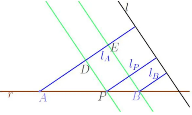
(7) Minimal distance from a point to n lines.. 41. Let us now check that the rate of change of SP , with respect to A, is constant: SA − SP SA − (P Q + P R) = AP AP SA PQ PR = − − AP AP AP SA PQ SA (P B) = − − AP AP (AB)(AP ) SA SB (AP ) SA (P B) = − − P A (AB)(AP ) (AB)(AP ) SA (AB) − SB (AP ) − SA (P B) = (AB)(AP ) SA (AB − P B) − SB (AP ) = (AB)(AP ) SA (AP ) − SB (AP ) = (AB)(AP ) SA − SB = . AB −SB is a constant, in other words, Note that SA , SB and AB are fixed, then SAAB −SP the quotient SAAP is the same for all P on AB.. Let us suppose now that the rate of change of SP with respect to A is constant for all P on AB (in the case of m given lines). Set k=. SP − SA SB − SA = , AP AB. where SA and SB are the sum of the distances from A and B to the m lines (respectively). If we consider one more line, l, and take lA and lB to be the distances from A to l and from B to l, respectively (see Figure 8), we get: (SB + lB ) − (SA + lA ) SB − SA lB − lA lB − lA = + =k+ . AB AB AB AB −lA Note that k + lBAB is again a constant. On the other hand, if lP is the distance from P to the new line, we have:. (SP + lP ) − (SA + lA ) SP − SA lP − lA lP − lA = + =k+ . AP AP AP AP We have to proof that lB − lA lP − lA = . AB AP. (∗).

(8) 42. M. Acosta, C. Mejı́a and C.W. Rodrı́guez. Figure 8: Distances from A, B and P to the added line l.. Now we draw parallel lines to l through P and B respectively (see Figure 8), those lines cut the orthogonal to l from A in D and E respectively. We can say, based on the fundamental theorem of proportionality (see [3]), that 4ADP and 4AEB are similar and therefore AD AE = . AP AB |lP −lA | AE But, AD and AB = AP = AP change is constant for all P .. |lB −lA | AB ,. which prove (∗). Consequently, the rate of. Now we are ready to prove proposition 1, using lemma 1.. Proof of proposition 1. Based on lemma 1, we say that the graph of SP when P is on AB is a segment; it is easy to see that if P varies along r, SP is continuous and therefore the graph of SP is a polygonal line with n vertices corresponding to the intersection of r with the given lines (see Figure 9). Furthermore, we can claim that if P moves away from the extremal intersection points, SP increases, and thus the polygonal line is open. Consequently, the polygonal line must have at least a minimum on one of its vertices..

(9) Minimal distance from a point to n lines.. 43. Figure 9: Polygonal line correspond to SP , with P in r.. To see what happens with SP as P varies on all the plane, we can vary the auxiliar line r parallely to itself, generating an infinity of polygonal lines, one for each position of r. On each one of these polygonal lines, SP reaches a minimum value when P is on the intersection of r with some given line, and therefore, if the minimum of SP on the plane exists, it must be a point M on some of the given lines. Thus, M ∈ l1 ∪ l2 ∪ · · · ∪ ln , in this way, we can consider the function SP restricted to the union l1 ∪ l2 ∪ · · · ∪ ln . Each line li intersects at least another given line (because not all lines are parallel). Thus, for li we can argue as we have done for r and the graph of SP . For P restricted to li , this graph is a polygonal line up-opened with vertices corresponding to the intersection points of li with all the other given lines. This polygonal line contains at least one minimizer Mi , with Mi ∈ li ∩ lj , and this is true for all j = 1, 2, · · · , n, j 6= i. Then, we have to examine at most n polygonal lines, each one corresponding to one of the given lines, and therefore the minimum of SP will be min{SM1 , SM2 , · · · , SMn }, and it is clearly placed on one of the intersection points Mi . Consequently the function SP reach its minimum on one of the intersection points of the given lines. As we said in the introduction, SP does not necessarily reach its minimum value at a single point; it could happen that SP reaches its minimum value at all points on an entire line, on a segment or even on a plane region. We will discuss these cases in a second paper..

(10) 44 4. M. Acosta, C. Mejı́a and C.W. Rodrı́guez. Conclusions. We solved the problem M IN using CABRI II plus in two ways: to represent instances of the problem and to compute the solution-set of those instances. The software allowed us to consider a huge number of instances, and the huge number of experiments we performed, allowed us to detect useful regularities in the solution-sets we computed. Then, we could propose a suitable conjecture which, with some work, could be formally proved. Although our solution is not new, we claim that our experimental approach is of interest and could be used for research and education. References [1] Borwein, J., et al. Experimentation in mathematics, computational paths to discovery. A. K. Peters. USA, 2004. [2] Baccaglini-Frank, A., and Mariotti, M.A. Conjecturing and Proving in Dynamic Geometry: the Elaboration of Some Research Hypotheses. In Proceedings of the 6th Conference on European Research in Mathematics Education, Lyon, January 2009 [3] Moise, E., and Downs, F. Jr. Geometrı́a Moderna. Fondo Educativo Interamericano, S.A. Massachusetts, 1964. [4] Mongomery, D., Peck,E., and Vining, G. Introducción al Análisis de Regresión lineal. Alay Ediciones, S.L. México, 2002. [5] Barbara, R. The Fermat-Torricelli Points of n Lines. The Mathematical Gazette, Vol. 84, No. 499, pp. 24-29, Mar., 2000 Authors’ address Martı́n E. Acosta — Escuela de Matemáticas, Universidad Industrial de Santander, Bucaramanga-Colombia e-mail: martin@matematicas.uis.edu.co Carolina Mejı́a — Departamento de Matemáticas, Universidad Nacional de Colombia, Bogotá-Colombia e-mail: caromejia77@gmail.com Carlos W. Rodrı́guez — Escuela de Matemáticas, Universidad Industrial de Santander, Bucaramanga-Colombia e-mail: cwrodriguez@matematicas.uis.edu.co.

(11)