Cumulative degradation in estuaries: contribution of individual species to community recovery

Texto completo

(1)See discussions, stats, and author profiles for this publication at: https://www.researchgate.net/publication/263278749. Cumulative degradation in estuaries: Contribution of individual species to community recovery Article in Marine Ecology Progress Series · June 2014 DOI: 10.3354/meps10904. CITATIONS. READS. 0. 37. 5 authors, including: Silvia de Juan. Simon F. Thrush. Pontifical Catholic University of Chile. University of Auckland. 35 PUBLICATIONS 377 CITATIONS. 281 PUBLICATIONS 10,010 CITATIONS. SEE PROFILE. SEE PROFILE. Judi E. Hewitt. Andrew M Lohrer. National Institute of Water and Atmospheric …. National Institute of Water and Atmospheric …. 216 PUBLICATIONS 6,841 CITATIONS. 75 PUBLICATIONS 1,606 CITATIONS. SEE PROFILE. SEE PROFILE. Some of the authors of this publication are also working on these related projects: The breathing seascape: resolving ecosystem metabolism and habitat-function relationships across coastal habitats View project Valuation and monitoring marine and coastal ecosystem services in Iberoamerican countries View project. All content following this page was uploaded by Silvia de Juan on 25 March 2016. The user has requested enhancement of the downloaded file..

(2) This authors' personal copy may not be publicly or systematically copied or distributed, or posted on the Open Web, except with written permission of the copyright holder(s). It may be distributed to interested individuals on request. MARINE ECOLOGY PROGRESS SERIES Mar Ecol Prog Ser. Vol. 510: 25–38, 2014 doi: 10.3354/meps10904. Published September 9. Cumulative degradation in estuaries: contribution of individual species to community recovery Silvia de Juan1, 2,*, Simon F. Thrush1, Judi E. Hewitt1, Jane Halliday1, Andrew M. Lohrer1 1. National Institute of Water and Atmospheric Research, PO Box 11-115, Hamilton, New Zealand Present address: Center for Marine Conservation, Pontificia Universidad Católica de Chile, Las Cruces, Chile. 2. ABSTRACT: To investigate the influence of macrofaunal species on recovery in soft-sediment habitats, a multi-site defaunation experiment was conducted in intertidal sandflats in Mahurangi Harbour, New Zealand. Paired treatment and control plots were monitored for 394 d after defaunation, and the recovery trajectories of individual species and their relationships with environmental factors were evaluated over time. Recruitment events were not apparent drivers of recovery, as we observed a massive recruitment of some species by Day 203, but the abundance of these individuals largely decreased by the end of the experiment, regardless of location in the estuary or hydrodynamics. Multiple regression models revealed highly variable responses, but suggested that several factors including sediment type and post-settlement species interactions contributed to species persistence in recovering plots. Juveniles generally settled at sites where adults from the same taxa occurred in the ambient community, suggesting local settlement patterns. Populations of functionally important surface deposit feeders and suspension feeders, including the large bivalves Austrovenus stutchburyi and Macomona liliana, failed to recover at most sites. The latter is likely one of the major drivers of divergence between disturbed and control plots in this experiment. The generally slow recovery dynamics, the degree of divergence of recovering communities and the failure of some key functions to recover have important implications for the response trajectories of coastal benthic communities subjected to increasingly frequent disturbance. KEY WORDS: Defaunation · Benthic recovery · Recovery dynamics · Functional traits · Macrofauna · New Zealand Resale or republication not permitted without written consent of the publisher. INTRODUCTION Ecosystem responses to disturbance can operate at different scales, with local disturbances having effects at the habitat and patch scales and broad-scale disturbances causing changes in community state at regional scales. Cumulative disturbances thus create a mosaic of patches with different community assemblages linked by recovery time and disturbance intensity (Zajac 2008). As the scale of disturbance increases and ecological fragmentation intensifies, there is loss of ecological connectivity and a reduction in potential sources of colonists to stimulate recovery as the disturbance wanes (Thrush et al.. 2008, de Juan et al. 2013). If disturbance persists, and time/space between events is not sufficient for complete recovery, the potential exists for broad-scale community homogenisation (Fahrig 2003). Central to the resilience of ecosystems to such disturbances are community and species recovery dynamics (Thrush et al. 2009). Empirical estimation of recovery rates is a pressing issue due to the growing use of models (parameterised by expert judgement, not necessarily empirical data) to predict community recovery as tools for ecosystem management (Teck et al. 2010). Disturbance-recovery experiments provide valuable information on the processes that determine the responses of ecosystems to changes in the distur-. *Corresponding author: [email protected]. © Inter-Research 2014 · www.int-res.com.

(3) Author copy. 26. Mar Ecol Prog Ser 510: 25–38, 2014. bance regime (Thrush et al. 2009). They also provide information on the drivers of recovery rates and the types of recovery trajectories. Post-disturbance recovery processes are generally a mix of biotic and abiotic interactions, strongly influenced by the source and transport of colonists from surrounding habitats, post-settlement habitat selection and species interactions (Pearson & Rosenberg 1978, Thrush et al. 2013). To date, numerous studies on the recovery of soft-sediment benthic communities have indicated the importance of local habitat features (Norkko et al. 2010); however, the role of larger-scale processes is difficult to assess, as definitive recovery experiments would have to encompass the habitat heterogeneity and other sources of natural variability in each area (Thrush et al. 2013). For example, the abundance patterns of the species interacting during the recovery can fluctuate linked to direct biotic interaction, i.e. competition for resources, indirect interactions mediated by the roles that organisms play in modifying disturbed habitats or simply by variable local environmental conditions (Montserrat et al. 2008, Norkko et al. 2010, Van Colen et al. 2012). Recovery dynamics are a product of species-specific biological traits (Norkko et al. 2010) and are often non-linear, with the high natural variability of benthic communities influencing the degree of divergence from pre-disturbance states (Thrush et al. 2008). The immigration of adult colonists into disturbed patches is an important mechanism of recovery in benthic sediment systems (Thrush et al. 2003), although the timing of disturbance relative to the availability of juvenile recruits settling from the water column also plays a role, particularly as the area of the disturbed patch increases (Whitlatch et al. 1997). It is now recognised that key properties of ecological communities, including recovery dynamics, can only be understood by placing the species within their spatial and temporal environmental context (Loreau et al. 2003). Changes in species assemblages after disturbance may have important consequences for ecosystem functioning (Van Colen et al. 2012). Soft sediments are complex systems where organisms play key functional roles (Lohrer et al. 2004), by bioturbating, irrigating and stabilising sediments and influencing organic matter remineralisation and nutrient regeneration (Solan et al. 2004, Thrush et al. 2006, Lohrer et al. 2010). However, not all species make equal contributions to functioning (Solan et al. 2004), and the significance of disturbance will depend on the individual species’ responses (Thrush et al. 2009). Despite the recognised importance of biodiversity loss on ecosystem functioning, few studies have ana-. lysed the functional implications of species loss in a disturbance-recovery context (Lohrer et al. 2010, Villnäs et al. 2013). Understanding the roles of key species within ecosystems is essential for predicting wider consequences of disturbance and species− environment interactions that might control recovery patterns (Norkko et al. 2010). The monitoring of the recovery of a set of defaunated plots across an estuary, conducted by Thrush et al. (2008), demonstrated the importance of both physical (hydrodynamics and habitat) and metacommunity connectivity in affecting the differences in recovery rates between sites. The experiment revealed that despite half of the sites recovering in terms of taxonomic richness, most of the communities in the disturbed plots did not match ambient communities after 394 d. Moreover, massive recruitment of some species did not result in long-term persistence or any lasting contribution to recovery. These findings triggered a more detailed examination into community recovery dynamics; here we focussed on recovery trajectories of individual species and functional traits, addressing the following questions: (1) Among 3 forms of trajectories (overshooting, transience or not recovering to ambient abundances), do individual species present the same form of trajectory at each site? (2) Do sets of species sharing a trajectory form also share a common set of dispersal characteristics or recruitment timing? (3) Is any lack of consistency in recovery of species among sites driven by local abundances or environmental factors? (4) Are the communities recovering their key functions? (5) Is the recovery of functional traits more consistent across time and space than the recovery of individual species? In order to address these questions, we examined recovery trajectories of macrofaunal species over time and their variability with respect to abiotic and biotic factors. We discuss our results in the context of the consequences of recovery dynamics on the functioning of ecosystems.. MATERIALS AND METHODS Defaunation experiment The experiment was conducted in Mahurangi Harbour, a 24.6 km2 harbour situated on the east coast of the North Island, New Zealand (Fig. 1). The 7 exper-.

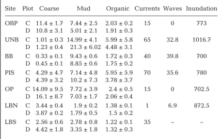
(4) 27. Author copy. de Juan et al.: Species recovery dynamics in estuaries. Fig. 1. Study area in New Zealand (North Island), including a detailed map of Mahurangi Harbour with the position of the 7 experimental sites: Opposite Bradleys Point (OBP), upper Ngaio Bay (UNB), Brown’s Bay (BB), Puka Puka Inlet South (PIS), Oaua Point (OP), Lagoon Bay North (LBN), Lagoon Bay South (LBS). imental sites were located on intertidal flats around the harbour, where sediments varied from fine mud in the upper sections of the estuary to coarse sand near the estuary entrance (sites ordered from upper to lower estuary: OBP, UNB, BB, PIS, OP, LBN and LBS). The intertidal sites also varied in macrobenthic community structure and hydrodynamics (Thrush et al. 2008). Three pairs of defaunated and control plots, each 6.25 m2 and separated by about 5 m, were established at the mid-tide level at each site. To defaunate the plots, the sediment surface was covered with black polythene sheets weighted with concrete paving (methodology described by Thrush et al. 1996). This experiment started on 24–25 November 2004, and the polythene sheets were left to smother the sediment until 11–12 January 2005 (detailed methodology in Thrush et al. 2008). Immediately after removal of the plastic cover, samples were taken to verify that complete defaunation had occurred. The plots were sampled 8 times: 1, 13, 24, 43, 86, 148, 203 and 394 d after the defaunated plots were uncovered. The sampling dates corresponded to summer (Days 1, 13 and 24), autumn (Days 43 and 86), winter (Day 148), spring (Day 203) and summer. again (Day 394). On each sampling date, macrofauna were sampled in each plot with 13 cm diameter × 15 cm depth cylindrical cores (n = 3). Core samples were sieved with a 500 µm mesh, sorted in the laboratory, identified to the lowest possible/practical taxonomic level and counted. Two additional small cores (1.5 cm diameter × 2 cm depth) were collected per plot on each sampling occasion, to measure organic content and sediment grain size.. Physical site characteristics All sampling sites were in sheltered locations with low wave energy (Table 1). The sediment composition of the sites varied; UNB was the muddiest and OBP had the highest gravel and shell hash content. The organic content ranged from an average of 1.3% at the exposed LBS site to 4.5% at the muddy, protected UNB site (Fig. 1, Table 1). Initial comparison of sediment composition and organic content of the sediments at the paired defaunated and control plots showed that defaunation of the plots did not significantly change these parameters in comparison to ambient site conditions..

(5) Author copy. 28. Mar Ecol Prog Ser 510: 25–38, 2014. Table 1. Mean ± SD of the percentage sediment composition in the defaunated (D) and control (C) plots at each site. Measures were obtained on Days 1, 86 and 394. Percentage of sand is not included in the table and is Sand = 100 – Coarse – Mud. Average hydrodynamics at each site include tidal currents (cm s−1), waves (cm s−1) and inundation (daily minutes). Sites as in Fig. 1. ples at each time (i.e. Day 1 to Day 394). The distance from the centroids of defaunated and control groups of samples provided a measure of changes in the similarity between plots. Site Plot Coarse Mud Organic Currents Waves Inundation In order to investigate the contribuOBP C 11.4 ± 1.7 7.44 ± 2.5 2.03 ± 0.2 15 0 773 tion of individual species to recovery D 10.8 ± 3.1 5.01 ± 2.1 1.91 ± 0.3 dynamics, we selected those species UNB C 1.01 ± 0.3 14.99 ± 4.1 5.99 ± 5.8 65 32.8 1016.7 that determined variability in similarD 1.23 ± 0.4 21.3 ± 6.02 4.48 ± 3.1 ity between defaunated and control BB C 0.33 ± 0.1 9.43 ± 0.6 1.72 ± 0.3 40 39.8 700 plots and between consecutive times D 0.45 ± 0.1 8.85 ± 0.6 1.75 ± 0.2 over the course of the experiment. PIS C 4.29 ± 4.7 7.14 ± 4.8 5.95 ± 5.9 70 35.6 780 Twenty-five taxa contributed up to D 4.39 ± 3.2 10.2 ± 7.3 3.78 ± 3.7 60% of the dissimilarity between OP C 14.09 ± 9.5 7.72 ± 3.9 2.4 ± 0.5 15 0 702.5 D 16.1 ± 8.7 7.03 ± 1.7 2.06 ± 0.4 sites, plots or times (SIMPER, Clarke LBN C 3.44 ± 0.4 1.9 ± 0.2 1.38 ± 0.1 1 6.9 872.5 & Warwick 1994). Abundance data D 3.87 ± 0.2 1.79 ± 0.5 1.5 ± 0.2 from these taxa were plotted to deterLBS C 2.56 ± 0.6 2.78 ± 0.8 1.22 ± 0.1 35 – – mine their temporal trajectories at D 4.42 ± 1.8 3.35 ± 1.8 1.32 ± 0.3 defaunated and control plots and to categorise species as overshooting, transient or not recovering. A subset of 14 taxa was selected as temporal patterns in The currents in the estuary are mainly controlled variability in abundance were identified as ‘overby tides, and the waves are primarily generated by shoot’ (i.e. higher abundance at defaunated plots in a wind. The principal tidal currents flow up and down specific time) or ‘transient’ behaviour (i.e. temporal the main channel and decline in strength with disincrease of abundance at defaunated and sometimes tance from the channel. Tidal currents were estialso at control plots). Finally, taxa that caused more mated as depth-averaged velocity for a spring tide than 5% of the difference in similarity between plots derived from a layered 3-dimensional hydrodynamic at any particular site at the end of the experiment model of the harbour and the surrounding area (Old(394 d after defaunation) were identified with SIMman & Black 1997). Inundation and waves were PER. From this analysis, 10 taxa had higher average measured using a DOBIE wave gauge. Average abundance in control plots and were considered to immersion times (inundation) were calculated for have not recovered (Table 2). each site and are expressed as minutes, and the waves To assess the significance of taxonomic variability are expressed as orbital velocity cm s−1 (Thrush et al. between defaunated and control plots over time, we 2000). Prior to analysis, we grouped the sites by conperformed a model-based analysis of multivariate sidering their ecological connectivity (i.e. the likeliabundance. We used the R package mvabund that hood of dispersal of colonists between them given fits a generalised linear model (GLM) to multivariate hydrodynamic flow patterns and physical barriers). abundance data (Wang et al. 2012). The multivariate Well-connected sites were grouped together: locaabundance data corresponded to the 14 taxa identition 1 comprised sites OBP and UNB, location 2 had fied as overshoot and/or transient. The explanatory site BB only, location 3 comprised sites OP and PIS, variables were site, included to assess potential difand location 4 comprised sites LBN and LBS (Fig. 1). ferences across locations, and the interaction of time Sites in the same group were not necessarily the and treatment to assess variability between plots closest together in physical straight-line distance. over time (species abundance ~ site + treatment × time; treatment: defaunated and control plots). A negative-binomial regression was specified for this Temporal dynamics in community recovery data set. The multivariate test statistic was based on patterns the likelihood ratio, taking into account the correlation between response variables. An adjusted pA principal coordinates analysis (Anderson & Willis value was calculated for each taxon with a step-down 2003), based on Bray-Curtis similarity with square Monte Carlo resampling algorithm with 500 resamroot transformation, provided an ordination of sam-.

(6) Author copy. de Juan et al.: Species recovery dynamics in estuaries. 29. Table 2. Transient (T), overshoot (O) or not recovering (N) taxa. In brackets: days of the transient/overshoot event. Additional data: sites where temporal patterns were detected, the day of recruitment and adult and larval dispersal. Amphipoda (Amp), Bivalvia (Biv), Cnidaria (Cni), Crustacea (Cumacea, Cum, and Decapoda, Dec), Gasteropoda (Gas) and Polychaeta (Pol). Orbinidae includes Orbinia papillosa and Scoloplos cylindrifer. Site names as in Fig. 1 Taxon. Temporal patterns. Sites. Adult mobility. Larval dispersal. Pol Biv Pol. Aonides trifida Theora lubrica Boccardia syrtis. O (24−43) O (86) O (24−394) T (43−86). OBP, LBS UNB OBP, UNB, PIS, OP, LBN, LBS BB. Limited Limited Sedentary. No Pelagic Pelagic. Pol. Nicon aestuariensis. O (86−203) T (86−203). OBP UNB, BB, PIS. Days 86−148, wide recruitment. Motile. Pelagic. Biv. Arthritica bifurca. O (148) LBN T (148−203) UNB, OP N UNB. Days 148−203, selected sites. Limited. Limited. Pol. Heteromastus filiformis. O (394) UNB T (148−203) BB, OP, LBS N OBP, BB, PIS. Days 148−203, selected sites. Motile. Pelagic. Cum Pol Dec Gas Pol Amp. Colurostylis lemurum Glycinde trifida Hemiplax hirtipes Notoacmea scapha Orbinidae Paracalliope spp.. T (203) T (148−203) T (24−43) T (148) T (148−203) T (13). LBS all sites PIS OBP BB OP. Day 203, selected sites Days 148−203, wide recruitment − Day 148, selected sites − Day 13, selected sites. Motile Motile High Limited Limited Motile. No Pelagic Pelagic Pelagic Pelagic No. Biv. Austrovenus stutchburyi. T (203) N. UNB, OP BB, PIS, OP, LBN. Days 148−203, wide recruitment. Motile. Pelagic. Pol. Exogoninae. T (203) N. LBS PIS, LBN, LBS. Day 1−13, wide recruitment. High. No. Cni Pol Pol Biv Biv Biv. Anthopleura aureoradiata Cossura sp. Euchone sp. Macomona liliana Nucula hartvigiana Paphies australis. N N N N N N. OBP, PIS, OP, LBN UNB BB, LBN, LBS OBP, UNB, BB, LBS OBP, BB, PIS, OP, LBS OBP. − − Day 1−13, selected sites − Day 1−13, wide recruitment −. Sedentary Limited Sedentary Limited Limited Motile. Pelagic No No Pelagic Pelagic Pelagic. ples. Residual vs. fits and Q-Q plots were visually inspected to check for the adequacy of the data structure.. Effects of biotic and abiotic factors on the recovery dynamics of the species To assess the effects of biotic and abiotic factors on recovery for individual overshoot, transient and nonrecovering taxa from the defaunated plots, we used GLMs, and when non-linear effects (i.e. splines) were detected for any variable we used generalised additive models (GAMs; Hastie & Tibshirani 1986). These models were performed with R program v.2.11.0 (www.r-project.org). The dependent variables were the abundance of selected taxa in defaunated plots (average of the 3 replicates) at all sites and times. The predictors included local sediment. Recruitment. Day 86, selected sites Days 24−86, wide recruitment. (mud, sand, coarse sand and organic content) and hydrodynamic (waves, tidal currents and inundation) variables; location as a categorical variable; and time as a continuous variable (1, 13, 24, 43, 86, 148, 203 and 394 d after defaunation). Ambient abundance, estimated using the average abundance in the paired control plots, was also included as a predictor to assess the relationship between variability in the abundance of defaunated and control plots over time. When relevant, potential positive or negative species interactions were included as predictors, using the abundance of identified facilitating or inhibiting species in defaunated plots at each time. In general, the presence of tubeworms facilitates settlement for many species, while the presence of some large fauna like gastropods or decapods disturbs the sediment surface and inhibits juveniles and small individuals (Callaway 2006, Hewitt & Cummings 2013). The connectivity distance to the nearest long-term.

(7) Author copy. 30. Mar Ecol Prog Ser 510: 25–38, 2014. population (i.e. determined from continuous quarterly monitoring initiated in July 1994) was available for some of the most abundant taxa and, in these cases, it was also included in the analysis to assess potential source−sink dynamics within the harbour. Dispersal traits of adult organisms were defined as highly motile, motile, limited motility and sedentary; we also considered pre-settlement dispersal of pelagic eggs and larvae related to recovery potential of the plots. Dispersal traits were treated as qualitative information for the interpretation of the results. Co-linearity diagnostics were examined to ensure that highly correlated environmental variables were not included in the final models (Belsley et al. 1980). As a result, sand content was excluded from the analyses as it was highly correlated with the mud content. A quasi-Poisson regression was specified for both the GLM and the GAM. The adequacy of the selected error structures was assessed with visual inspection of residuals vs. fits plots. The spline effects included in the GAM were restricted to n/3 knots. The backwards selection criteria were Akaike’s information criterion for the GLM and GCV (General CrossValidation Score) for the GAM (Guisan et al. 2002).. Recovery of ecosystem functions We used biological traits relevant for characterising the function of food processing and bioturbation, viz. feeding mode and living position. Traits were assigned to all but rare species (defined as those with an average abundance at all times across sites <15 individuals). Species with the same attributes were pooled into functional groups. The final functional groups used were predators, suspension feeders, surface deposit feeders, surface deposit feeders that subduct particles, subsurface deposit feeders (above 2 cm), deep deposit feeders (below 2 cm) and subsurface or deep deposit feeders that move particles to the sediment surface. A multivariate GLM (mvabund R package, Wang et al. 2012) was also applied to the functional traits data set, following the same criteria used for the species abundance multivariate GLM. SIMPER analysis was performed to identify the functional groups responsible for the differences between defaunated and control plots at each site towards the end of the experiment (Days 203 and 394). The abundance of functional groups in defaunated plots was regressed against local sediment variables, hydrodynamic factors, location, ambient abundance of the corresponding functional group (i.e. abundance in the paired control plots) and time as a con-. tinuous variable. The GLM and GAM followed the same criteria and assumptions explained for the regression models performed with individual species’ abundance.. RESULTS Temporal and spatial variability in recovery patterns: species dynamics Over the course of the experiment, the defaunated and control communities converged in ordination space, but after 394 d, the defaunated plot communities had not completely recovered to resemble their respective ambient community types (Fig. 2). At 203 d after defaunation, the average similarity between defaunated plots across sites was higher than the average similarity between defaunated and control plots at each site. A multivariate GLM was fitted to the overshoot and transient taxa (Table 2). The overall test showed significant differences between sites, treatments (i.e. defaunated and control plots), times and the interaction of treatment and time (Table 3a). Most of the transient taxa were only significantly affected by time (e.g. Glycinde trifida, Nicon aestuariensis); overshoot taxa generally showed a significant interaction between treatment and time (e.g. Arthritica bifurca, Heteromastus filiformis); transient taxa that did not recover at the end of the experiment showed significant differences between treatments interacting with time (e.g. Austrovenus stutchburyi, Exogoninae). Other taxa were found in very low densities at most sites and only significant differences between sites were detected (e.g. Colurostylis lemurum, Hemiplax hirtipes, Theora lubrica; Table 3a). Generally, the selected taxa were more abundant in control plots, but the overall abundance in both disturbed and control plots was low (Fig. 3a). Six taxa exhibited overshoot behaviour (Table 2); these were generally low in abundance in control plots and, after the overshoot event, decreased in abundance or even became absent from the defaunated plots by Day 394 (Fig. 4). However, for 2 of the 6 cases (the polychaetes Boccardia syrtis and H. filiformis), the overshoot event lasted until the end of the experiment at several sites, increasing the dissimilarity between plots. The 6 overshoot taxa did not generally show overshoot behaviour at all sites, with 4 of these taxa exhibiting transient behaviour at other sites (generally in the same time period, Table 2). Another 8 taxa exhibited transient behaviour at 1 or.

(8) de Juan et al.: Species recovery dynamics in estuaries. 31. Author copy. more sites (Table 2), mostly between Days 148 and 203 (Fig. 4), suggesting that this was a period of general recruitment, when the similarity between defaunated and control plots increased (Fig. 2). Some of the transient taxa, such as G. trifida or Notoacmea scapha, were rare or absent from both defaunated and control plots outside this recruitment event. Other ‘low abundance’ taxa, such as C. lemurum or Paracalliope spp., only recruited to selected sites where the taxa were previously present in the ambient community. Exogoninae and A. stutchburyi were the only transients in defaunated plots that were relatively common (mean abundance >1 ind. core−1 in control plots; Figs. 3a & 4). Ten taxa that had higher abundances in controls were responsible for > 5% of the dissimilarity between control and defaunated plots at 1 or more sites 394 d after defaunation (Table 2, Fig. 4). These taxa generally failed to recover at 3 or more sites. Most of the taxa not recovering either did not have a recruitment event over the course of the experiment (13 mo) or recruited early in the experiment. However, 3 of the taxa that did not recover (A. bifurca, A. stutchburyi and H. filiformis) recruited at Days 148 to 203, but by Day 394, their abundance had decreased in the defaunated plots at some sites (Table 2).. Effects of biotic and abiotic factors on species recovery dynamics. Fig. 2. Principal coordinates analysis (PCO) of species abundance data at control (circles) and defaunated (squares) plots from Days 1 to 394 after defaunation. Sites, 1: OBP, 2: UNB, 3: BB, 4: PIS, 5: OP, 6: LBN, 7: LBS (full site names in Fig.1). Distances among centroids of defaunated/control groups are given in brackets. The multiple correlation models explained over 85% of the variance for A. stutchburyi but only 10% for B. syrtis (Table 4). Correlation models could only be fitted to 8 taxa, as most of the data exhibited left-skewed distributions. Several taxa recruited early in the experiment yet failed to settle in the defaunated plots (Table 2). Of the early recruiters,.

(9) Mar Ecol Prog Ser 510: 25–38, 2014. Author copy. 32. Table 3. Analysis of deviance (Dev) for the (a) multi-taxa and (b) functional traits data sets. Results for each variable are also provided, with an adjusted p-value (adjusted for multiple testing). ns: non-significant effects. Treatment: defaunated and control plots, DF: deposit feeders, SF: suspension feeders. Dev a) Multi-taxa Taxon Intercept Aonides trifida Arthritica bifurca Austrovenus stutchburyi Boccardia syrtis Colurostylis lemurum Exogoninae Glycinde trifida Heteromastus filiformis Hemiplax hirtipes Nicon aestuariensis Notoacmea scapha Paracalliope spp. Theora lubrica b) Functional traits Functional group Intercept Deep DF Deep-to-surface DF Predator SF Subsurface DF Surface DF Surface-to-deep DF. 156.5 7.21 24.94 11.15 19.37 35.08 20.29. 18.63. 164.5 60.48 35.08. 63.66. Site p(>Dev). < 0.01 ns ns < 0.05 < 0.01 < 0.01 < 0.01 ns < 0.01 < 0.01 ns ns ns < 0.01. < 0.01 < 0.01 < 0.01 ns ns ns ns < 0.01. Treatment Dev p(>Dev). 133.6 59.7 31.62. 19.69. 424.4 46.03 3.16 16.31 113.99 37.60 145.93 61.36. Exogoninae had wide recruitment and were common in control sites; however, abundance in the defaunated plots was related to location and time (see also Table 3a). Nucula hartvigiana and Euchone sp. failed to recover at 5 sites, and were responsible for > 5% of the dissimilarities between plots at 3 sites, by the end of the experiment. Euchone sp. was almost absent from all defaunated plots and exhibited significant interactions with time and organic content (Table 4). Several taxa that exhibited larval/post-larval dispersal had recruitment events more than 3 mo after defaunation, but their abundance in treatments had decreased by the end of the experiment (Table 2). G. trifida and N. aestuariensis had wide recruitment, but their abundances were strongly related to sediment type and local ambient abundance, which was generally low outside the main recruitment events, or the presence of tubeworms in the case of G. trifida. The abundance of A. stutchburyi, despite being common in ambient communities, was transient in the defaunated plots where its abundance was positively affected by the presence of large infauna and tubeworms in a non-linear fashion, and with the ambient. < 0.01 ns ns < 0.01 ns ns < 0.01 ns ns ns ns < 0.01 ns ns. < 0.01 < 0.01 < 0.05 < 0.01 < 0.01 < 0.01 < 0.01 < 0.01. Dev. Time p(>Dev). 154.3 35.26. 30.86 30.43 30.63. 88.7 34.31 17.04 17.70 9.68. < 0.01 ns ns < 0.01 ns ns ns < 0.01 < 0.01 ns < 0.01 ns ns ns. < 0.01 ns < 0.01 < 0.01 < 0.01 ns < 0.05 ns. Treatment:time Dev p(>Dev). 185.0 16.32 55.07 45.51 49.74. 299.8 58.83 72.05 32.22 21.61 59.24 50.76. < 0.01 ns < 0.01 < 0.01 ns ns < 0.01 ns < 0.01 ns ns ns ns ns. < 0.01 ns < 0.01 < 0.01 < 0.01 < 0.01 < 0.01 < 0.01. abundance. H. filiformis was more abundant in the defaunated plots on several occasions (Table 2), but the only significant predictor for this species was mud content (Table 4).. Recovery of ecosystem functions The multivariate GLM of functional group abundance showed significant effects of site, treatment, time and the interaction of treatment and time (Table 3b, Fig. 3b). For most functional traits, the effect of treatment was time dependent (significant time × treatment interaction), while significant effects of site were only detected for deep, deep-to-surface and surface-to-deep deposit feeders (Table 3b). The functional groups responsible for dissimilarities between plots at the end of the experiment differed between sites (Fig. 5, Table 5). Surface-to-deep deposit feeders failed to recover at sites OBP and LBN, and densities in the defaunated plots were related to location and mud content in a non-linear fashion (Table 4). Surface deposit feeders failed to recover at.

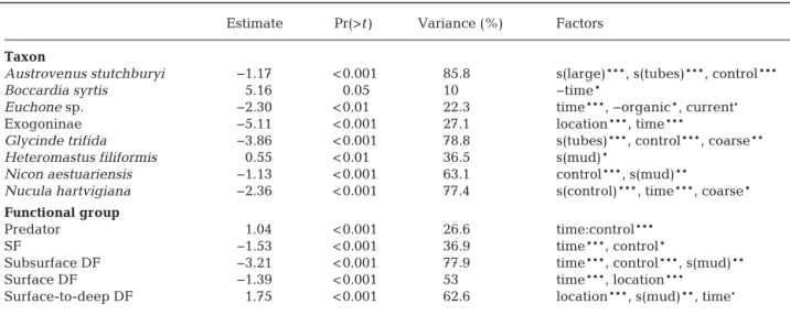
(10) 33. Author copy. de Juan et al.: Species recovery dynamics in estuaries. Fig. 3. Abundance of overshoot/transient taxa and functional groups against treatment groups (C: control, D: defaunated plots). Plots on the right are the residual vs. fits for the multivariate generalised linear model; the colours represent data from each variable (i.e. taxon or functional group). DF: deposit feeders, SF: suspension feeders. Table 4. Generalised linear and generalised additive models with the abundance of taxa and functional groups as response variables. Predictors: local physical variables, location, the abundance of the taxa/functional group in control plots and time since defaunation. Models for individual taxa also include the distance to the nearest long-term population and biotic interactions as the abundance of facilitating species (tubes: abundance of tube worms) or inhibitors (‘large’ infauna). ·p < 0.1, *p < 0.05, **p < 0.01 and ***p < 0.001. ‘−’: negative effects, s: spline. Taxa and functional groups without significant models are excluded. SF: suspension feeders, DF: deposit feeders Estimate. Pr(>t). Variance (%). Factors. Taxon Austrovenus stutchburyi Boccardia syrtis Euchone sp. Exogoninae Glycinde trifida Heteromastus filiformis Nicon aestuariensis Nucula hartvigiana. −1.17 5.16 −2.30 −5.11 −3.86 0.55 −1.13 −2.36. < 0.001 0.05 < 0.01 < 0.001 < 0.001 < 0.01 < 0.001 < 0.001. 85.8 10 22.3 27.1 78.8 36.5 63.1 77.4. s(large)***, s(tubes)***, control*** −time* time***, −organic*, current· location***, time*** s(tubes)***, control***, coarse** s(mud)* control***, s(mud)** s(control)***, time***, coarse*. Functional group Predator SF Subsurface DF Surface DF Surface-to-deep DF. 1.04 −1.53 −3.21 −1.39 1.75. < 0.001 < 0.001 < 0.001 < 0.001 < 0.001. 26.6 36.9 77.9 53 62.6. time:control*** time***, control* time***, control***, s(mud)** time***, location*** location***, s(mud)**, time·.

(11) Mar Ecol Prog Ser 510: 25–38, 2014. Author copy. 34. Fig. 4. Abundance (mean ± SD) of overshoot/transient or not recovering taxa in control (s) and defaunated plots (d) at selected sites from Day 1 to Day 394 after defaunation. First row: transient taxa; second row: overshoot taxa; third row: taxa that did not recover. Full site names in Fig. 1. 4 sites (OBP, PIS, OP and LBS; Fig. 5) and were related to time and location. Subsurface deposit feeders were in low abundance at all sites (Figs. 3b & 5), and densities in the defaunated plots were related to ambient abundances, time and mud content in a non-linear fashion. Predators generally recovered, and the abundance of this group was linked to a linear interaction between time and ambient abundance. Suspension feeders failed to recover at sites PIS, OP and LBN, and densities in the defaunated plots were mainly related to time. Correlation models could not be fitted to deep and deep-to-surface deposit feeders, as these groups exhibited low abundance and had left-skewed abundance data distributions. Deep deposit feeders were only detected in sufficient densities at UNB; this group failed to recover at this site (Fig. 5, Table 5).. DISCUSSION Despite the small size of the defaunated plots (6 m2) the failure of most species to settle caused differences between recovering and ambient communities that lasted until the end of the experiment (+ 394 d). There was no consistent set of species that recovered in abundance for which recovery was linked with dispersal traits or with timing of the recruitment event; in fact, successful early settlement did not necessarily lead to these species contributing to the long-term recovery of the plots. There was also only limited evidence of a consistent set of early settlers that conditioned sediment for later colonists, with the presence of tubeworms important for 2 species. Moreover, differences in recovery among sites did.

(12) de Juan et al.: Species recovery dynamics in estuaries. Author copy. 35. Fig. 5. Abundance of functional groups 394 d after defaunation. For each site, the abundances in control (c) and defaunated (d) plots are included in left and right plots, respectively. Data corresponds to the average abundance (± SD) of the 7 functional groups (group 7 only present at site UNB). DF: deposit feeders, SF: suspension feeders. Full site names in Fig. 1 Table 5. Contribution of the functional groups to differences between control and defaunated plots at the end of the experiment in each site. Data correspond to the % contribution to dissimilarity (diss) between plots, averaged from Days 203 and 394, and the plot with the higher average abundance in these times (C: control, D: defaunated). Data with the highest diss/SD are shown in bold. DF: deposit feeders, SF: suspension feeders. Full site names in Fig. 1 Functional group Deep DF Deep-to-Surface DF Predators SF Subsurface DF Surface DF Surface-to-deep DF. OBP. UNB. BB. PIS. OP. LBN. LBS. – 18.6 C 10.9 C 16.2 C 16.8%C 19.7 C 20.9 C. 29.2 C 19 D 14.4 D 9.1 D 6.7 C 11.5 C 10.2 D. – 16.4 D 20.1 D 10.3 C 18.4 C 11.6 C 23.2 D. – 12.9 D 10.7 D 30.8 C 5.8 C 22.9 C 8.4 C. – 16.4 D 14.9 D 22.2 C 4C 26.8 C 9.4 D. – 8.4 C 10.7 C 28.9 C 6.7 D 12.9 C 26.3 C. – 7.8 D 19.5 D 10.7 C 10.7 C 26.6 C 16.6 D. not appear strongly related to hydrodynamics or sediment characteristics. Although widespread recruitment events of many species did occur, abundances of most of these declined and disappeared from the defaunated plots,. and sometimes also from the ambient community, by the end of the experiment, with few exceptions like Boccardia syrtis that overshot at most sites until the end of the experiment. Most of the overshoot species did not appear to have long-term effects on.

(13) Author copy. 36. Mar Ecol Prog Ser 510: 25–38, 2014. recovery, and these species were generally observed at low densities outside the overshoot periods. Overshoot events were not generally consistent across sites, with only 2 species, the polychaetes B. syrtis and Glycinde trifida, demonstrating this at most sites. Interestingly, these 2 species were almost absent from ambient communities outside recruitment events. Abundances observed for Austrovenus stutchburyi in defaunated plots generally failed to recover back to ambient abundances, despite the fact that recruitment events were recorded at all sites. This bivalve species has widely dispersing larvae and is relatively large and mobile in adulthood (suggesting that it should have been able to immigrate across defaunated plot edges). However, limited mobility and context-dependent recovery rates have been recorded for this species in other parts of New Zealand (Hewitt & Cummings 2013). The case of Heteromastus filiformis was also unusual, as it is mobile throughout its life and a recruitment event occurred, yet it still failed to recover at some sites. At other sites, paradoxically, its abundance was higher in defaunated plots by the end of the experiment. Despite results reflecting the complexity of factors conditioning recovery, recruits generally stayed at sites where adults of their taxa occurred in the ambient community, suggesting habitat−species interactions. Some of the taxa that did not recover from defaunation after 394 d did not have a recruitment event during our sampling. For others, recruitment occurred but colonists were transients and did not persist in the defaunated plots. These results suggest that the timing of recruitment after disturbance is important for the recovery of a community. This implies that to estimate recovery rates we first need to understand the temporal dynamics of communities in a disturbance-recovery context. In intertidal soft-sediment habitats, bed load transport of post-larvae due to waves is important (Hewitt et al. 1997); however, in our sheltered sites it was not expected that this would make a major contribution to recovery, and this expectation was confirmed by the weak relationship between species abundance and hydrodynamic factors. While recovery of soft sediments is probably largely driven by the migration of organisms from neighbouring areas, in our study motility alone was of limited importance; rather, lack of recovery appeared to link to low densities of some of these mobile species in the ambient communities (e.g. G. trifida, Nicon aestuariensis, Hemiplax hirtipes and Colurostylis lemurum).. Although sediment characteristics did not appear affected by the defaunation experiment (Thrush et al. 2008), abundances of Austrovenus in the recovering plots were positively related to the presence of other large infauna (e.g. large bivalves and decapoda). Early colonisers have been documented to influence the settlement of later arrivals through both resource competition or by the reworking of sediments (Lohrer et al. 2004, Van Colen et al. 2008). Conversely, removal of species that stabilise the sediment (like tubeworms) can also slow recovery (Thrush et al. 1996), and in our experiment, 2 species with harbourwide recruitment that failed to settle were linked to the density of tubeworms. Tubeworms can provide a stable habitat and a reduced risk of predation for larvae and juveniles (Callaway 2006), thus the settlement of some taxa might be conditioned by the prior recovery of tubeworm density. No single species at a site was driving recovery, and this pattern could be related to the high spatial heterogeneity and temporal variability in species richness observed in this estuary (de Juan & Hewitt 2014). Recovery after disturbance does not necessarily imply a return to a pre-stress community configuration, as numerous interacting factors during recovery can result in community divergence (Hobbs et al. 2009). The high natural variability might influence the divergence of recovery trajectories, as observed in our experimental sites more than a year after defaunation. However, it is the actual functional roles played by the species that would indicate the degree of divergence after disturbance (Mouillot et al. 2013). Taxa that failed to recover included large, longerlived bivalves, important bioturbators that play key roles in soft-bottom communities (Thrush et al. 2006). The functional groups that did not recover differed among sites, although differences between control and treatment plots were mostly due to surface deposit feeders, surface suspension feeders and surface-to-subsurface deposit feeders that failed to recover at 4, 3 and 2 sites, respectively. This is counter to a defaunation experiment conducted by Thrush et al. (1996) where recovering plots were mostly composed of surface organisms. In our study, surface organisms were generally abundant but appeared to recover more slowly than subsurface organisms despite the latter generally occurring in lower densities at most sites. This raises the question, is this slow recovery of surface deposit feeders a product of their higher baseline abundance? If verified, it would have important implications for the recovery of functions, as functionality is strongly.

(14) Author copy. de Juan et al.: Species recovery dynamics in estuaries. related to organism size and abundance. The influence of size and density could have important implications for the generally accepted importance of functional redundancy to ensure ecosystem resilience (Walker 1992). The failure of surface deposit feeders to recover at most sites has important ecological consequences, as these organisms provide important functions including bioturbation-mediated processes (Lohrer et al. 2004). In this same estuary, Lohrer et al. (2010) observed that the site with the highest bioturbation potential (dominated by large bivalves), exhibited the largest decline in functioning (nutrient fluxes) immediately after disturbance. Although the size of the organisms in the recovering plots was not assessed, the important functional roles of adult bivalves suggest that organism size is an important trait to include in future studies on benthic ecosystem recovery. In summary, a complex interplay of factors contributes to recovery in soft-sediments habitats and, as a result, recovery trajectories can be extremely variable. The regional species pool sets the stage by governing the colonists that are available to contribute to recovery. While the timing of disturbance relative to the species’ seasonal dynamics can be important, recruitment events alone may not drive recovery. The movement of mobile post-settled individuals also plays a role and, as time goes on, within-site biotic and abiotic interactions become more and more important (Montserrat et al. 2008, Thrush et al. 2013). Importantly, functional recovery may lag behind the degree of recovery indicated by community composition when organisms playing key roles for ecosystem functioning fail to recover, with consequent implications for the functional performance of these estuarine systems under increasing disturbance regimes. Slow and unpredictable recovery from small-scale disturbances compromises resilience and increases the potential for transitions into undesirable, functionally degraded states. It is therefore necessary to incorporate the reality of slow and unpredictable recovery in sand-flat systems into ecosystem-based management thinking. Acknowledgements. We thank the large number of NIWA staff past and present that participated in the arduous fieldwork. Approval to conduct this experiment in Mahurangi Harbour was granted by the Auckland Regional Council (now Auckland Council). The research was funded by FRST C01X0501 and NIWA under Coasts and Oceans Research Programme 3 (2012/13 SCI). S.d.J. was funded by a postdoctoral mobility grant from The Spanish Ministry of Education (Programa nacional de movilidad de recursos humanos del Plan Nacional I+D+i 2008-2011).. 37. LITERATURE CITED Anderson MJ, Willis TJ (2003) Canonical analysis of principal coordinates: a useful method of constrained ordination for ecology. Ecology 84:511−525 Belsley DA, Kuh E, Welsch R (1980) Regression diagnostics: identifying influential data and sources of collinearity. Wiley, New York, NY, p 25−49 Callaway R (2006) Tube worms promote community change. Mar Ecol Prog Ser 308:49−60 Clarke KR, Warwick RM (1994) Changes in marine communities: an approach to statistical analysis and interpretation. Natural Environment Research Council, Plymouth de Juan S, Hewitt JE (2014) Spatial and temporal variability in species richness in a temperate intertidal community. Ecography 37:183−190 de Juan S, Thrush SF, Hewitt JE (2013) Counting on β-diversity to safeguard the resilience of estuaries. PLoS ONE 8: e65575 Fahrig L (2003) Effects of habitat fragmentation on biodiversity. Annu Rev Ecol Evol Syst 34:487−515 Guisan A, Edwards TC Jr, Hastie T (2002) Generalized linear and generalized additive models in studies of species distributions: setting the scene. Ecol Model 157:89−100 Hastie T, Tibshirani R (1986) Generalized additive models. Stat Sci 1:297−318 Hewitt JE, Cummings VJ (2013) Context-dependent success of restoration of a key species, biodiversity and community composition. Mar Ecol Prog Ser 479:63−73 Hewitt JE, Pridmore RD, Thrush SF, Cummings VJ (1997) Assessing the short-term stability of spatial patterns of macrobenthos in a dynamic estuarine system. Limnol Oceanogr 42:282−288 Hobbs RJ, Higgs E, Harris JA (2009) Novel ecosystems: implications for conservation and restoration. Trends Ecol Evol 24:599−605 Lohrer AM, Thrush SF, Gibbs M (2004) Bioturbators enhance ecosystem function through complex biogeochemical interactions. Nature 431:1092−1095 Lohrer AM, Halliday J, Thrush SF, Hewitt JE, Rodil IF (2010) Ecosystem functioning in a disturbance-recovery context: contribution of macrofauna to primary production and nutrient release on intertidal sandflats. J Exp Mar Biol Ecol 390:6−13 Loreau M, Mouquet N, Holt RD (2003) Meta-ecosystems: a theoretical framework for a spatial ecosystem ecology. Ecol Lett 6:673−679 Montserrat F, Van Colen C, Degraer S, Ysebaert T, Herman PMJ (2008) Benthic community-mediated sediment dynamics. Mar Ecol Prog Ser 372:43−59 Mouillot D, Graham NJ, Villéger S, Mason NWH, Bellwood DR (2013) A functional approach reveals community responses to disturbances. Trends Ecol Evol 28:167−177 Norkko J, Norkko A, Thrush SF, Valanko S, Suurkuukka H (2010) Conditional responses to increasing scales of disturbance, and potential implications for threshold dynamics in soft-sediment communities. Mar Ecol Prog Ser 413:253−266 Oldman JW, Black KP (1997) Mahurangi estuary numerical modelling. NIWA Client Report, ARC60208/1. National Institute of Water and Atmospheric Research, Hamilton Pearson TH, Rosenberg R (1978) Macrobenthic succession in relation to organic enrichment and pollution of the marine environment. Oceanogr Mar Biol Annu Rev 16: 229−311.

(15) Author copy. 38. Mar Ecol Prog Ser 510: 25–38, 2014. Solan M, Cardinale BJ, Downing A, Engelhardt KAM, Ruesink JL, Srivastava DS (2004) Extinction and ecosystem function in the marine benthos. Science 306: 1177−1180 Teck SJ, Halpern BS, Kappel CV, Micheli F and others (2010) Using expert judgment to estimate marine ecosystem vulnerability in the California Current. Ecol Appl 20: 1402−1416 Thrush SF, Whitlatch RB, Pridmore RD, Hewitt JE, Cummings VJ, Wilkinson MR (1996) Scale-dependent recolonization — the role of sediment stability in a dynamic sandflat habitat. Ecology 77:2472−2487 Thrush SF, Hewitt JE, Cummings VJ, Green MO, Funnell GA, Wilkinson MR (2000) The generality of field experiments: interactions between local and broad-scale processes. Ecology 81:399−415 Thrush SF, Hewitt JE, Norkko A, Nicholls PE, Funnell GA, Ellis JI (2003) Habitat change in estuaries: predicting broad-scale responses of intertidal macrofauna to sediment mud content. Mar Ecol Prog Ser 263: 101−112 Thrush SF, Hewitt JE, Gibbs M, Lundquist CJ, Norkko A (2006) Functional role of large organisms in intertidal communities: community effects and ecosystem function. Ecosystems 9:1029−1040 Thrush SF, Halliday J, Hewitt JE, Lohrer AM (2008) The effects of habitat loss, fragmentation, and community homogenization on resilience in estuaries. Ecol Appl 18: 12−21 Thrush SF, Hewitt JE, Dayton PK, Coco G and others (2009). Forecasting the limits of resilience: integrating empirical research with theory. Proc R Soc Lond B Biol Sci 276: 3209−3217 Thrush SF, Hewitt JE, Lohrer AM, Chiaroni LD (2013) When small changes matter: the role of cross-scale interactions between habitat and ecological connectivity in recovery. Ecol Appl 23:226−238 Van Colen C, Montserrat F, Vincx M, Herman PMJ, Ysebaert T, Degraer S (2008) Macrobenthic recovery from hypoxia in an estuarine tidal mudflat. Mar Ecol Prog Ser 372:31−42 Van Colen C, Rossi F, Montserrat F, Andersson MGI and others (2012) Organism-sediment interactions govern post-hypoxia recovery of ecosystem functioning. PLoS ONE 7:e49795 Villnäs A, Norkko J, Hietanen S, Josefson AB, Lukkari K, Norkko A (2013) The role of recurrent disturbances for ecosystem multifunctionality. Ecology 94:2275−2287 Walker B (1992) Biodiversity and ecological redundancy. Conserv Biol 6:18−23 Wang Y, Naumann U, Wright ST, Warton DI (2012) mvabund — an Rpackage for model-based analysis of multivariate abundance data. Methods Ecol Evol 3: 471−474 Whitlatch RB, Hines AH, Thrush SF, Hewitt JE, Cummings V (1997) Benthic faunal responses to variations in patch density and patch size of a suspension-feeding bivalve. J Exp Mar Biol Ecol, 216(1–2):171–189 Zajac RN (2008) Macrobenthic biodiversity and sea floor landscape structure. J Exp Mar Biol Ecol 366:198−203. Editorial responsibility: Martin Solan, Southampton, UK. Submitted: October 18, 2013; Accepted: June 5, 2014 Proofs received from author(s): August 19, 2014.

(16)