The influence of superstructures on bright galaxy environments: clustering properties
12
0
0
Texto completo
(2) 2. Yaryura et al.. (Park & Choi 2009; Binggeli 1982; Donoso et al. 2006; Crain et al. 2009; White et al. 2010). The formation and evolution of systems that are embedded in superstructures could be conditioned by these large overdensities (Hoffman et al. 2007; Araya-Melo et al. 2009; Bond et al. 2010, and references therein). Galaxies within them also show different properties and spatial distributions (Einasto et al. 2003; Wolf et al. 2005; Haines et al. 2006; Einasto et al. 2007; Porter et al. 2008; Tempel et al. 2009; Fleenor & Johnston-Hollitt 2010; Tempel et al. 2011; Einasto et al. 2011). Recent galaxy redshift surveys (York et al. 2000; Colless et al. 2001) sample a sufficiently large volume to allow the study of galaxy formation and evolution from a statistical perspective and unveil its details with increasing confidence. The aim of this work is to use SDSS–DR7 catalogue (Abazajian et al. 2009) to study the influence of superstructures on galaxies. We will study the dependence of the clustering of faint galaxies (tracers, −21.0 < Mr < −20.5) around brighter galaxies (centres, −23.0 < Mr < −21.0) according to whether the centre galaxies are part of superstructures. In this work, we will analyse the clustering properties of galaxies located in large structures which are still undergoing a virialization process. Then we can study the differences in the small scale clustering of these galaxies compared to galaxies in the field. For this study, we use the superstructures identified by Luparello et al. (2011), dubbed Future Virialized Structures (FVS), identified in the SDSS–DR7 and Zapata et al. (2009) groups which will be used to characterize the virial mass of the groups which host our galaxies. This paper is organized as follows. In Section 2 we describe data collected for groups of galaxies and future virialized structures. We then analyse the clustering properties using the crosscorrelation function, as described in Section 3, and show results in Section 4. We summarize and discuss the results in Section 5.. 2 DATA AND SAMPLES 2.1 SDSS–DR7 Galaxy Catalogue The Sloan Digital Sky Survey (York et al. 2000) is one of the largest and most ambitious surveys carried out so far. It has deep multi– colour images covering more than one quarter of the sky, and spectra for about 930000 galaxies and 120000 quasars. It is one of the largest data sets produced and contains images, image catalogues, spectra and redshifts. In this work we use the Seventh Data Release (DR7, Abazajian et al. 2009), which is publicly available 1 . The spectroscopic galaxy catalogue comprises a footprint area of 9380 sq.deg. The limiting apparent magnitude for the spectroscopic catalogue in the r–band is 17.77 (Strauss et al. 2002). We use a more conservative limit of 17.5 to ensure completeness. Also, in order to avoid saturation effects in the photometric pipeline, we consider galaxies fainter than r = 14.5. The image deblending software often fragments images of bright galaxies with substructure, so our cuts prevent possible artifacts in the final catalogue 2 . 2.2 SDSS–DR7 Superstructures The maps of the Universe depict a complex network of filaments and voids (e.g. Einasto et al. 1996; Colless et al. 2001; 1 2. http://www.sdss.org/dr7 http://www.sdss.org/dr7/products/general/target quality.html. Jaaniste et al. 2004; Einasto 2006; Abazajian et al. 2009), where clusters of galaxies are preferentially located at the nodes of filamentary structures (Gonzalez & Padilla 2010; Murphy et al. 2011). This picture was possible only after extended galaxy surveys were completed, and it is also supported by numerical experiments consistent with the standard cosmological model (Frisch et al. 1995; Bond et al. 1996; Sheth et al. 2003; Shandarin et al. 2004). Large scale structures, which we will refer to as superstructures, have been studied with a variety of methods. The first statistical studies of superstructures were performed by linking Abell cluster positions (Zucca et al. 1993; Einasto et al. 1997). Later, the realization of wide-area surveys of galaxies with redshift as Las Campanas Redshift Survey (Shectman et al. 1996), the 2-degree Field Galaxy Redshift Survey (2dFGRS, Colless et al. 2001) and the Sloan Digital Sky Survey (SDSS, York et al. 2000; Stoughton et al. 2002), allowed the identification of superstructures directly from the large-scale galaxy distribution. Einasto et al. (2007) identified superclusters in the 2dFGRS using a density field method, and Costa-Duarte et al. (2011) studied the morphology of superclusters of galaxies in the SDSS. The largest catalogue of superclusters has been constructed by Liivamägi et al. (2012), who implemented the density field method on the SDSS–DR7 main and luminous red galaxy samples. In all cases, superclusters are operationally defined as objects within a region of positive galaxy density contrast, and thus are subject to a certain degree of arbitrariness in their detection. Within the ΛCDM Concordance Cosmological Model, an accelerated expansion dominates the present and future dynamics of the universe and thus determines the nature of gravitationally bound structures. Therefore, an alternative definition of these large-scale structures is that of overdense regions in the present-day universe that will become bound and virialized structures in the future. Thus, under the assumption that the luminosity is a somewhat unbiased tracer of mass on large scales, the integrated luminosity density of galaxies is commonly used as an indicator of mass density. Luparello et al. (2011) applies the luminosity density field method to identify FVS in large spectroscopic galaxy surveys. The identification procedure is based on the theoretical criteria of Dünner et al. (2006). Using numerical simulations, they establish the minimum mass overdensity neccesary for a structure to remain bound in the future. Luparello et al. (2011) use this mass overdensity criteria to calibrate the luminosity–density threshold, and identify superstructures as systems that are likely to evolve into virialized structures in the distant future, in the assumed cosmology. The catalogue of FVS was extracted from a volume-limited sample of galaxies from the SDSS–DR7, in the redshift range 0.04 < z < 0.12, with a limiting absolute magnitude of Mr < −20.47. The luminositydensity field is constructed on 1 h−1 Mpc cubic cells grid, applying an Epanechnikov kernel of r0 = 8 h−1 Mpc (equation 3 of Luparello et al. (2011)). The luminosity overdensity threshold is fixed at DT = ρlum /ρ̄lum = 5.5, and the structures are constructed by linking overdense cells with a simple version of a ”Friends of Friends” algorithm. In order to avoid contamination from smaller systems, they also assign a lower limit for the total luminosity of a structure at L struct > 1012 L⊙ . The main catalogue of superstructures has completness over 90 per cent and contamination below 5 per cent, according to calibrations made using mock catalogues. The volume covered by the catalogue is 3.17 × 10⁷ (h−1 Mpc)3 , within which 150 superstructures were identified, composed by a total of 11394 galaxies. FVS luminosites vary between 1012 L⊙ and ≃ 1014 L⊙ , and their volumes range between 102 (h−1 Mpc)3 and 105 (h−1 Mpc)3 . Because of the luminosity density field depen-.
(3) Galaxy clustering dence, Luparello et al. (2011) analysed 3 samples with different luminosity thresholds, dubbed S1, S2 and S3, described in table 1 of their paper. We will consider sample S2 in our analysis, which contains 89513 galaxies with Mr < −20.47 in the redshift range 0.04 < z < 0.12. 2.3 SDSS–DR7 Galaxy Groups The aim of this paper is to analyse the clustering of galaxies considering different samples. Some of these samples are selected taking into account the mass of the systems considered. To estimate the mass distributions of the samples we use the estimated mass of galaxy groups. The galaxy groups correspond to those identified in the SDSS galaxy catalogue presented by Zapata et al. (2009), extended to cover the SDSS–DR7. Zapata et al. (2009) identified groups using the same method as Merchan & Zandivarez (2005), with a ”Friends of Friends” algorithm, with a variable projected linking length and a fixed radial linking length. These were set by Merchan & Zandivarez to obtain a sample as complete as possible and with low contamination (95 per cent and 8 per cent, respectively). The catalogue contains 83784 groups with at least 4 members, and is limited to redshift z < 0.12. 2.4 Synthetic catalogue and simulation In order to test the procedures implemented in this work, we constructed a mock galaxy catalogue from a semi-analytic model of galaxy formation (GALFORM, Bower et al. 2008) applied to the Millennium simulation (Springel et al. 2005), which adopts a ΛCDM concordance cosmological model. The semi-analytic model of galaxy formation collects information from the merger trees extracted from the simulation, and generates a population of galaxies within the simulation box. The mock catalogue is set up to mimic the geometry of the SDSS–DR7 footprint and reproduces the dilution in the number of galaxies with redshift.. 3 METHOD The clustering of galaxies is analysed using the two–point correlation function. Early studies of the spatial distribution of galaxies using this technique were presented by Peebles (1980). The two– point correlation function, ξ(r), is defined as the excess of the probability, δP, of finding a galaxy, defined as tracer, at a given distance from another galaxy, dubbed the centre. Thus, δP = ng (1 + ξ(r))dV,. (1). where dV is a volume element and ng is the mean number density of tracer galaxies. There are several estimators of this function (Kerscher et al. 2000) that compute this probability by counting object pairs. In this work, we use one of the most commonly used estimators to determine the cross–correlation function, as defined by Davis & Peebles (1983): ξ=. D1 D2 NR1 NR2 − 1, R 1 R 2 N D1 N D2. (2). where Di D j is the average number of object pairs and Ri R j is the average number of pairs in a random sample. NDi and NRi represent the number of objects in the data catalogue and in the random sample, respectively. The random sample is generated with the same geometry as the real catalogue using the same angular and radial selection functions. In particular, the advantage of this estimator. 3. is that if the sample D1 has few objects, R1 can be selected to be larger than D1 , and thus minimize the noise in the ξ calculation. Although there are more accurate estimators, like the one defined by Landy & Szalay (1993), differences between both estimators are negligible due to the large volume size of the SDSS (e.g. Paz et al. 2011). In galaxy redshift catalogues, where the distance is estimated using the spectroscopic redshift which includes a peculiar velocity component, the three dimensional distribution of galaxies is affected by distortions in the line of sight. To take this into account we estimate the correlation function ξ(σ, π), as a function of the projected (σ) and line of sight (π) distances. As these distortions in redshift space occur only in the radial direction, we implement the inversion presented by Saunders et al. (1992) to obtain the spatial correlation function ξ(r) from ξ(σ, π). We integrate along the line of sight to obtain the projected correlation function Ξ(σ): Z ∞ Z ∞ p Ξ(σ) = 2 ξ(σ, π)dπ = 2 ξ( σ2 + y2 )dy. (3) 0. 0. In this work we use σ = 0.3 and π = 0.3 Mpc as lower integration limits for this equation, and σ = 30 and π = 30 Mpc as upper limits. We use diferent binning schemes for ξ(σ, π) according to the size of each sample, being the number of bins in the range 13 to 19. Then, we can directly estimate the real space correlation function (ξ(r)) by the inversion of Ξ(σ) assuming a step function Ξ(σi ) = Ξi in bins centered in σi and interpolating between r = σi values (equation 26 of Saunders et al. 1992): q 2 2 1 X Ξ j+1 − Ξ j σ j+1 + σ j+1 − σi . (4) ξ(r) = − ln q π j>i σ j+1 − σ j σ + σ2 − σ2 j j i. This equation is a simple and direct way to invert the projected correlation function. In addition, we also compute the correlation function in redshift space, ξ(s), where s2 = x2 + y2 − 2xycosθ is the redshift-space distance; and x and y are the line of sight distances to each object of the pair, with angular separation given by θ = σ/y. ξ(s) contains information about the peculiar velocities of the galaxies in the sample.. 4 RESULTS We select galaxies which are members of the superstructures defined by Luparello et al. (2011) to construct the samples of galaxies in FVS, while we select galaxies which are members of the SDSS–DR7 galaxy catalogue but are not members of FVS for the samples of galaxies outside superstructures. To analyse the clustering properties of both samples, we measure the cross–correlation function, using faint galaxies with luminosity −21.0 < Mr < −20.5 as tracers. In both cases we select galaxies with luminosity −23.0 < Mr < −21.0 as centres. The centre and tracer galaxies are above the luminosity limit for the volume limited sample of the SDSS–DR7 galaxy catalogue. In Section 4.1, we analyse the correlation functions around centre galaxies inside and outside FVS. The difference in the clustering of faint galaxies around bright galaxies is not only produced by the selection of galaxies according to their FVS membership, but also is related to other processes that occur on smaller scales. In particular, the luminosity of galaxies is known to correlate with the clustering amplitude of galaxies (Alimi et al. 1988; Zehavi et al. 2005; Swanson et al. 2008; Wang et al. 2011; Zehavi et al. 2011;.
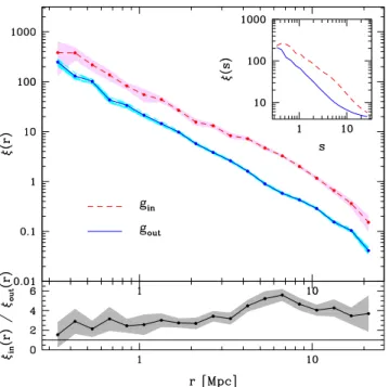
(4) 4. Yaryura et al. galaxies −23.0 < −23.0 < −23.0 < −23.0 < −23.0 < −23.0 <. Mr Mr Mr Mr Mr Mr. < −21.0 < −21.0 < −21.0, same luminosity dist. < −21.0, same mass dist. < −21.0, same mass and luminosity dists. < −21.0, same mass and luminosity dists., in mock. > 8 members and same mass distribution > 8 members and same mass dist., in mock. galaxies in Groups. Groups. g gG gL gG M gG ML gG ML − mock G8M G8M − mock. Nin. Nout. 5563 2013 5102 1765 1765 5550. 33306 4603 30526 3900 3316 8711. 509 708. 1829 2145. Table 1. Description of samples of galaxies or groups used as centres in the computation of ξ(r). Each name indicates objects (galaxies or groups) inside and outside FVS by the ”in” and ”out” sufixes, respectively. When indicated, subsamples are selected so that the distributions of galaxy luminosities or group masses inside and outside FVS are comparable. The last two columns indidate the number of objects in each centre sample.. Ross et al. 2011). There is also evidence of the dependence of clustering with dark matter host mass (Zehavi et al. 2012). Then, in order to disentangle and quantify the contribution of luminosity and mass to the total correlation amplitude, we will analyse the effect of equating luminosity and mass distributions on the correlation signal in Sections 4.2 and 4.5. In order to perform this analysis, we will use different samples of centre galaxies selected according to different properties. In Table 1 we give a brief summary of the samples (galaxies or groups) which are used as centres in the computation of correlation functions. Each sample name is used for two samples: one for galaxies located in a FVS, which we denote with the ”in” subindex, and the other for galaxies which are not part of any FVS, identified with the ”out” subindex. The number of objects in each sample is also given in Table 1. In Section 4.1 we will analyse samples gin and gout , which contain bright galaxies (−23.0 < Mr < −21.0) of the SDSS catalogue. In Section 4.2 we will analyse samples gL which are defined from the g samples, but with the additional restriction that their luminosity distributions are comparable. In Section 4.3 we introduce the SDSS–DR7 galaxy groups in the analysis and we separate the groups located inside and outside FVS. Then, we define the samples gG selecting bright galaxies contained in these groups. To analyse effects on the galaxy selection, in Section 4.4 we define new samples from the group catalogue. We redefine the group samples of Section 4.3 in order to have the same group virial mass distributions. The samples denoted by gG M are obtained by selecting the bright galaxies contained in these groups. To further constrain our samples, in Section 4.5 we redefine the samples gG ML by adding the condition that the bright galaxies located in groups with the same mass distributions also have the same luminosity distributions, i.e, the gG ML samples contain bright galaxies with the same luminosity distributions located in groups with the same mass distributions. In Section 4.6 we select galaxy groups with at least 8 members, and then divide them according to whether they are located in FVS or not, and we make their mass distributions similar by selectively limiting the sample. In this case, to define the G8M samples we select geometrical centres of groups instead of the bright galaxies, so that we can use virial mass estimated for groups to uncover mass effects. In Section 4.7 we define the same samples as gG ML and G8M but taken from a mock catalogue. We name these samples as gG ML−mock and G8M −mock respectively, and use them to test the reproducibility of our results by current models for structure formation.. Figure 1. Cross–correlation functions of SDSS–DR7 galaxies for the g samples. The dashed lines correspond to galaxies in sample gin and the solid lines correspond to galaxies in sample gout .. 4.1 Clustering of faint galaxies around bright galaxies Fig. 1 shows the cross–correlation functions for samples gin and gout , i.e., all galaxies in the luminosity range −23.0 < Mr < −21.0. The dashed curves show the results obtained for the sample of galaxies in FVS, gin , while the solid lines show the correlation function obtained for the sample of galaxies not contained in FVS. The shadowed regions indicate cosmic variance estimates computed using Jackknife statistics over the FVS catalogue. The number of Jackknife realizations is equal to the number of FVS in each case. As can be seen from this plot, the probability excess of finding a centre–tracer pair of galaxies is higher for the sample of galaxies contained in FVS than that corresponding to the sample of galaxies outside FVS, i.e. the clustering of galaxies is greater when they are contained in superstructures. A difference in clustering on large scales (two–halo term) is expected given the selection criteria applied to the samples. Galaxies in the same range of brightness are.
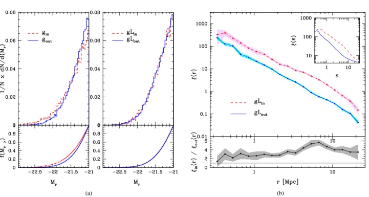
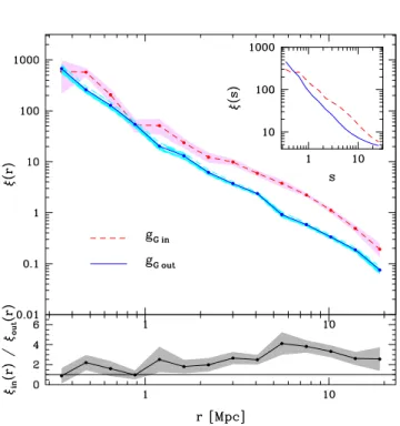
(5) Galaxy clustering. (a). 5. (b). Figure 2. (a) Luminosity distributions. The left panel corresponds to the g samples and the right panel shows the luminosity distributions of the new samples (gL), defined to have the same luminosity distributions. In both cases, the dashed curves correspond to the centres galaxies belonging to FVS while the solid curves correspond to the centre galaxies outside FVS. The bottom panels show the empirical cumulative luminosity distributions for each case. (b) Cross– correlation functions of SDSS–DR7 galaxies for gL samples. The dashed lines correspond to galaxies in FVS and the solid lines correspond to galaxies outside FVS. Both samples have the same luminosity distributions.. more clustered if they are in FVS, on small and large scales (one– halo term and two-halo term). From Fig. 1 it is evident that the clustering of galaxies is greater for galaxies located within the FVS, which suggests the possibility that the formation histories of galaxies and their collapse, are strongly influenced by the large-scale environment. However, this signal should be taken as an upper limit for this effect. Indeed, other correlations caused by differences in the galaxy selection of the two samples could diminish the clustering difference. In order to quantify how this selection affects the results, we will consider a number of restrictions on galaxy properties, using other samples of Table 1.. 4.2 Clustering of faint galaxies around bright galaxies: uncovering galaxy luminosity effects The clustering of galaxies is known to depend on the luminosity of galaxies (Alimi et al. 1988; Zehavi et al. 2005; Swanson et al. 2008; Wang et al. 2011; Zehavi et al. 2011; Ross et al. 2011). Therefore we will analyse how this dependence affects the previous results. The median luminosity of gout galaxies is fainter than that of gin galaxies. This means that centres outside FVS are typically less luminous, and therefore their clustering amplitude would be lower than that of galaxies which are located in FVS due to this. To rule this out, we define samples gLin and gLout from the original g samples, trimming objects so that the final luminosity distributions are similar. This proccess is made by comparing the original luminosity distributions and then randomly removing objects from either of these two samples. This removal is proportional to the differences between the distributions at a given luminosity. We progressively discard objects until the two distributions are reasonably similar.. The left panel of Fig. 2(a) shows the luminosity distributions of the original g samples, where dashed curves correspond to sample gin and solid curves correspond to the sample gout . In the right panel we show the luminosity distributions of the new samples gL, trimmed to have the same luminosity distributions, where dashed curves correspond to gLin and solid curves correspond to gLout . The bottom panels show the empirical cumulative luminosity distributions for each case. We estimate the cross–correlation functions for both gL samples, shown in Fig.2(b). Here we use the same line style coding of Figure 1. As can be seen there is a statistically significant difference between the clustering amplitudes of both samples, being greater for galaxies contained within FVS. This signal is observed at all scales including small scales (one–halo term), suggesting an effect of the surrounding FVS on the galaxy environment. This signal is, by construction of the samples gL, independent of the luminosity of centre galaxies but it still may depend on the mass of haloes they inhabit.. 4.3 Clustering of faint galaxies around bright galaxies: Galaxies in groups In this section we study the origin of the previous signal of different clustering amplitude for galaxies of equal luminosity inside and outside FVS, focusing on the virial mass of the host groups of galaxies, which can be interpreted as probing larger, but still intermediate scale structures. We select galaxy groups for which we have estimates of their mass. As a first step, we compare the cross– correlation function of galaxies in groups, distinguishing between groups that are located inside and outside FVS. To this end we use the SDSS–DR7 galaxy group catalogue described in Section 2.3..
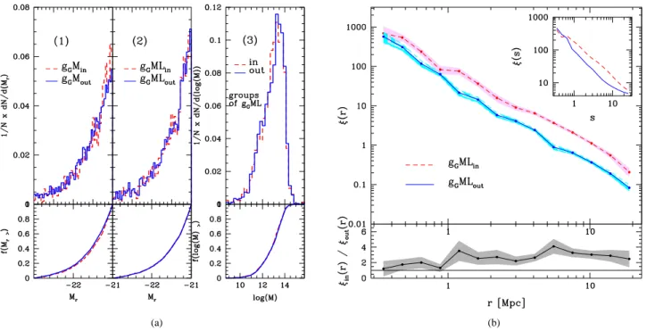
(6) 6. Yaryura et al. From the latter two samples of groups, we define two samples of centre galaxies contained in these groups: one with galaxies in groups belonging to FVS (gG Min ) and the other one with galaxies in groups outside FVS (gG Mout ). Fig. 4(b) shows the cross–correlation functions of these samples. The dashed lines correspond to the sample gG Min while the solid lines correspond to the sample gG Mout . As can be seen from this figure, the correlation function amplitudes differ only slightly in the inner regions (r . 1 Mpc). This is a similar behaviour to that observed in the case of centre galaxies in groups (−23.0 < Mr < −21.0), selected without restrictions in group mass.. 4.5 Clustering of faint galaxies around bright galaxies: combined effects from luminosity and mass. Figure 3. Cross–correlation functions of galaxies in groups (gG samples). The dashed lines correspond to galaxies in gGin sample and the solid lines correspond to galaxies in gGout sample.. We define two new samples of centre galaxies contained in these groups, one with groups belonging to the FVS (gGin ) and the other one with groups that do not belong to any FVS (gGout ). Galaxies are again restricted to luminosities within −23.0 < Mr < −21.0, as in the previous analyses. For a more direct comparison, we use the same tracer sample as in previous sections. The cross–correlation functions of the centre–tracer pairs for both samples are shown in Fig. 3. The dashed curves correspond to sample gGin , while the solid curves correspond to galaxies in sample gGout . 4.4 Clustering of faint galaxies around bright galaxies: uncovering dark matter mass effects In this section, we analyse the possible effects coming from differences in the mass of the groups where the centre galaxies reside. Therefore, we repeat the analysis performed for the luminosity dependence (Section 4.2), redefining instead samples with the same mass distributions. To determine the mass distributions we use the SDSS–DR7 galaxy groups catalogue described in Zapata et al. (2009) as in the previous section. We define two samples of galaxy groups, one with groups belonging to FVS and other one with groups outside FVS. The median of the mass distribution of the galaxy groups that do not belong to FVS corresponds to a lower value than the median of the mass distribution of groups inside FVS. We adjust these samples and redefine two new samples of groups, trimmed so that their mass distributions are similar. The left panel of Fig. 4(a) shows the mass distributions for the original samples, where dashed lines correspond to groups located in FVS and solid lines correspond to groups outside FVS. With the same line style coding, the right panel shows the mass distributions of the new samples, redefined to have the same mass distributions. The bottom panels show the empirical cumulative mass distributions for each case.. In this section we analyse how the luminosity and mass dependence of clustering affect the previous results. To do this, we repeat the previous process restricting samples to have comparable galaxy luminosity and host group mass distributions simultaneously. The left panel of Fig.5(a) shows the luminosity distributions of the centre galaxies of the samples gG M described in previous section, which are defined to have similar mass distributions. The dashed curves correspond to galaxies in the sample gG Min while the solid curves correspond to galaxies in the sample gG Mout . The middle panel of Fig. 5(a) shows the luminosity distributions of the new samples (gG MLin and gG MLout ) defined by equating the luminosity distributions of the previous samples (same line coding). The bottom panels show the empirical cumulative distributions for each case. It is important to ensure that the mass distributions of the hosts of centre galaxies remain similar once the luminosity distributions are trimmed to be comparable. The right panel of Fig.5(a) shows the mass distributions of the groups of the samples gG ML. The line coding is the same as in the previous plots. From this plot we can corroborate that the mass distributions of both samples remain comparable. The bottom panel shows the empirical cumulative mass distributions for each case. Thus, we obtain two samples of centre galaxies with similar luminosity distributions, populating groups with comparable mass distributions. One of these samples contains galaxies in groups which are members of FVS (gG MLin ), and the other comprises galaxies in groups away from FVS (gG MLout ). The cross–correlation functions of the centre– tracer pairs for both samples are shown in Fig.5(b). The dashed curves correspond to galaxies in sample gG MLin , while the solid curves correspond to the galaxies in sample gG MLout . From this figure we conclude that at small scales, the amplitudes of the clustering of both samples are slightly different, but within a 1-σ uncertainty.. 4.6 Clustering of faint galaxies around centres of groups: G8M samples. In this section we analyse the group–galaxy cross–correlation function, considering faint galaxies as tracers, as in the previous cases, but in this case selecting geometrical centres of groups instead of the brightest group galaxies, i.e, we study the dependence of the clustering of faint galaxies around centres of groups, using the same faint galaxy tracers as previous sections. To this aim, we define two samples of groups with at least 8 galaxy members, one with groups located inside FVS and another with groups outside FVS. To make a direct comparison, we define two new samples equating the mass distributions of the above.
(7) Galaxy clustering. (a). 7. (b). Figure 4. (a) Mass distributions of galaxy groups. The left panel corresponds to the original samples of galaxy groups, where the dashed lines are the groups located inside FVS and the solid lines are the groups located outside FVS. The right panel corresponds to the new samples of groups redefined to have the same mass distributions. The bottom panels show the empirical cumulative mass distributions for each case. (b) Cross–correlation functions of galaxies in groups for gG M samples. The dashed lines correspond to galaxies in groups of gG Min sample and the solid lines correspond to galaxies in groups of gG Mout sample. Both samples have the same mass distributions.. (a). (b). Figure 5. (a) The left panel shows the luminosity functions of the centre galaxies in groups, where these groups have the same mass distributions (i.e., luminosity distribution of samples gG M). The middle panel shows the luminosity distributions of the centre galaxies of the new samples redefined to have the same mass and luminosity distributions (gG ML). The right panel shows the mass distributions for groups composing samples gG ML. This plot is to be sure that the mass distributions do not change when we adjusted the samples to have the same luminosity distributions. The bottom panels show the cumulative functions for each case. As the previous cases, in all panels the dashed lines indicate groups located in FVS, while the solid lines indicate groups located outside FVS. (b) Cross–correlation functions of galaxies in groups for gG ML samples. The dashed lines correspond to galaxies in sample gG MLin and the solid lines correspond to galaxies in sample gG MLout . Both samples have the same luminosity and mass distributions..
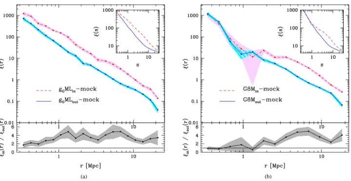
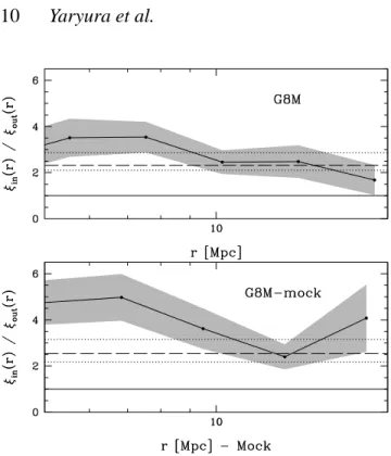
(8) 8. Yaryura et al.. mentioned samples. The left panel of the Fig.6(a) shows the mass distributions of groups with at least 8 members, where the dashed lines correspond to groups that are members of FVS and the solid lines correspond to groups that are not members of FVS. The right panel shows the mass distributions of the new samples, redefined to have the same mass distributions. The line coding is the same as in the previous sections. The bottom panels show the empirical cumulative mass distributions for each case. To determine the cross–correlation functions we use faint galaxies as tracers (defined in Section 4.1) and the geometrical centres of groups as centres (G8M). Fig.6(b) shows the cross– correlation functions for samples G8M. As in previous cases, the dashed lines correspond to centres of groups in sample G8Min , while the solid lines correspond to centres of groups in sample G8Mout . As can be seen, there is no differences between the two correlation functions at scales of up to 2 h−1 Mpc when virial masses are considered.. 4.7 Mock: gG ML − Mock and G8M − Mock samples. In order to assess the reproducibility of our previous results by current models for structure formation, we perform a similar analysis on a mock galaxy catalogue. We use the mock catalogue described in Section 2.4, which implements a semi–analytic model of galaxy formation in a ΛCDM cosmological framework. We have identified both FVS and groups in this mock galaxy catalogue using the same procedures than that used in the SDSS–DR7. We estimate the cross–correlation functions for the corresponding samples to Section 4.5 and 4.6. The samples gG ML − mock are selected from the mock catalogue following the same steps and taking into account the same restrictions implemented on the observational data (Section 4.5). Fig. 7(a) shows the corresponding cross–correlation functions, using the same line coding as in previous plots. Similarly, the samples G8M − mock are defined from the mock catalogue under the same conditions mentioned in Section 4.6. Fig. 7(b) shows the cross–correlation functions obtained from these samples. As can be seen in these figures, the correlation functions estimated in mock catalogues are consistent with the results from observational data.. 4.8 Discussion The mass contained in the FVS is likely to form part of a virialized structure in the future, but can also be considered to be part of the original overdensity when it started its collapse in the past. Therefore, this mass can be used as a proxy for the equivalent peak height of the FVS. We will test this by comparing the amplitude of the correlation function at large separations, r > 10 h−1 Mpc, with that expected for peaks corresponding to the FVS masses. Fig. 8 shows the ratios between the correlation functions around objects inside and outside FVS, for G8M and G8M − mock samples. These ratios can be compared with the ratio between the corresponding bias factors expected for objects of the mass of the FVS and that of the centres outside superstructures. In order to do this, we need to obtain an estimate of the groups outside superstructures, and also of the FVSs. For the former, we use their virial masses, and for the latter, we measure their total luminosities and adopt the average mass–to–light ratio for large–scale structures, < M/L >= 577 M⊙ /L⊙ , given by Tinker et al. (2010). The bias factors for the groups and FVSs are then obtained using the fitting formula given by Tinker et al. (2010), based on Sheth et al. (2001). The resulting ratio, ∼ 2.4 ±0.3, is shown as a solid horizontal long-. dashed line. As can be seen, in both real and mock data, these estimates are consistent with the ratios between the measured correlation functions. Errors are represented by the horizontal dotted lines, located at the 16th and 84th percentils of the distribution of bias values for the set of haloes considered. The amplitude of the correlation function at large separations for objects lying inside FVS, is consistent with that expected for a structure of the mass of the FVS, and not with that expected for their virial mass. The interpretation for this result is that the positions of the centres used for the measurement of the correlation function trace, on average, the location of the overdensity of the FVS. We test this hipothesis by measuring the centre of mass of the FVS using low and high mass groups living in them (we define low mass groups as M < 1013 M⊙ , and high mass groups as M > 1014 M⊙ ). We find that the centres of mass are similar to within 1.1 h−1 Mpc, which explains the small effect of the centres on the amplitude of the correlation function at large separations. We also measure the ratio between the correlation functions of these low and high mass groups living inside FVS. If they only traced the overdensity of the FVS, this ratio should be consistent with 1. Figure 9 shows this ratio in the top panel, confirming our hypothesis. The lower panel shows the same ratio taking as centres all the low and high mass groups in the SDSS, and as can be seen, the ratio is significantly lower than 1, on average, as expected for this ratio in the case that the groups trace their own lower or higher overdensity corresponding to their lower or higher masses (respectively), rather than that of an FVS. As a final test, we also divided the sample of FVS in two, one for low and another for high FVS mass samples, and calculated the cross-correlation function between groups populating these samples and tracer galaxies. As before, we ensure that the mass distributions of the groups are similar, to avoid the possible influence of the group mass on the amplitude of the correlation sample (even though we already showed that this is negligible when groups reside in an FVS). We find indications that the clustering for groups in higher mass FVSs is higher, also lending more support to the results shown previously. Regarding smaller scales, those corresponding to the one–halo term, our analysis indicates that the differences in the clustering amplitude, taking into account whether galaxies reside in FVS or not, are the sum of several contributions. We identified at least two sources that may be responsible for these differences, i.e., the different clustering amplitude due to galaxy luminosity and galaxy host mass selection effects. We acknowledge that there may be other sources that contribute to this deviation related to the selection of distinct large–scale environments. However, our analysis indicates that deviations originated on those sources are not statistically significant, pointing at a scenario where the FVS environnment has no measurable effect on the 1-halo clustering.. 5 CONCLUSIONS In this work we present a detailed analysis of cross–correlation of faint and bright galaxies and its dependence on large–scale structures. To this end, we use the properties of galaxy groups to characterize local environments (Zapata et al. 2009), and the properties of future virialized structures (Luparello et al. 2011) as proxies of large scale environments. We distinguish between galaxies belonging to FVS and galaxies outside FVS in a volume limited sample up to z = 0.12. At large scales, the amplitude of the two.
(9) Galaxy clustering. (a). 9. (b). Figure 6. (a): The left panel shows the mass distributions of groups with at least 8 members. The right panel shows the mass distributions of the new samples of groups with at least 8 members, adjusted to have the same mass distributions (G8M). The bottom panels show the empirical cumulative mass distributions for each case. In all panels, the dashed lines correspond to groups inside FVS and the solid lines correspond to groups outside FVS. (b): Group–galaxy cross–correlation functions for samples G8M, where the groups have at least 8 members and have the same mass distributions. The dashed lines correspond to groups in sample G8Min and the solid lines correspond to groups in sample G8Mout .. (a). (b). Figure 7. (a): Mock: Cross–correlation functions of galaxies in groups. The dashed lines correspond to galaxies in sample gG MLin − mock and the solid lines correspond to galaxies in sample gG MLout − mock. Both samples have the same luminosity and mass distributions. (b): Mock: Group–galaxy cross–correlation functions, where the groups have at least 8 members and have the same mass distributions. The dashed lines correspond to groups in sample G8Min − mock and the solid lines correspond to groups in sample G8Mout − mock..
(10) 10. Yaryura et al.. Figure 8. Ratio of the real–space correlation functions of galaxies inside and outside FVS, for samples G8M (upper panel) and G8M − mock (bottom panel), in solid lines, with uncertainties given by the shaded regions. The long-dashed horizontal lines shows the expected value for this ratio using the estimated FVS mass as that of the original overdensity that will eventually give rise to a virialized structure, and that of the centres outside FVS. The dotted lines enclose the 1 − σ confidence values for this theoretical ratio.. point cross–correlation function of bright and faint galaxies is significantly larger when the bright galaxies reside in FVS. At small scales, where the clustering cross–correlation signal is dominated by the local environment, the results inside and outside FVS are slightly different. In order to disentangle local and large scale contributions to the observed clustering, we have considered subsamples where the galaxy luminosity, and host group mass distributions are forced to be similar. Once these restrictions have been implemented, the resulting correlation functions show statistically negligible differences. In order to asses the reproducibility of these results within current models for structure formation, we have performed a similar analysis using a semi–analytic implementation in a ΛCDM cosmological model. We have determined bright–faint galaxy cross– correlations taking into account the local and global environment using groups and FVS in a similar fashion as performed in the observations. By considering subsamples with similar galaxy luminosity and host group mass distributions we determine that the cross–correlations dependence on large-scale structures is consistent with the dependence found in the observations. This analysis suggests that the resulting behaviour of the cross–correlation clustering of bright and faint galaxies on large scale structures is a generic feature of galaxy clustering in hierarchical scenarios and our current understanding of galaxy formation scenario. We studied the amplitude of the correlation function at large separation for centres inside and outside FVS, comparing them to that expected from the theory. We find that objects in FVS show a large–scale clustering consistent with that of an overdensity of the mass of the FVS in which they reside. These objects trace, on average, the centre of mass of the FVS, explaining this effect. Furthermore, for groups inside FVS, the amplitude of the correlation function at two–halo term separations does not seem to depend on group mass. This dependence is more clear when considering all the groups in the SDSS. In a forthcoming paper we will assess the properties of galaxies in systems residing inside and outside FVS.. ACKNOWLEDGEMENTS. Figure 9. Upper panel: cross-correlation function ratio, ξin−low−mass (r)/ξin−high−mass (r), for groups living inside FVS. Low mass corresponds to groups with M < 1013 M⊙ while high mass corresponds to groups with M > 1014 M⊙ . Bottom panel: same as top panel, but for all the groups in SDSS separated in low and high mass samples.. This work was partially supported by the Consejo Nacional de Investigaciones Cientı́ficas y Técnicas (CONICET), and the Secretarı́a de Ciencia y Tecnologı́a, Universidad Nacional de Córdoba, Argentina. NP was supproted by Fondecyt Regular #1110328. Funding for the SDSS and SDSS–II has been provided by the Alfred P. Sloan Foundation, the Participating Institutions, the National Science Foundation, the U.S. Department of Energy, the National Aeronautics and Space Administration, the Japanese Monbukagakusho, the Max Planck Society, and the Higher Education Funding Council for England. The SDSS Web Site is http://www.sdss.org/. The SDSS is managed by the Astrophysical Research Consortium for the Participating Institutions. The Participating Institutions are the American Museum of Natural History, Astrophysical Institute Potsdam, University of Basel, University of Cambridge, Case Western Reserve University, University of Chicago, Drexel University, Fermilab, the Institute for Advanced Study, the Japan Participation Group, Johns Hopkins University, the Joint Institute for Nuclear Astrophysics, the Kavli Institute for Particle Astrophysics and Cosmology, the Korean Scientist Group, the Chinese Academy of Sciences (LAMOST), Los Alamos National Laboratory, the Max-Planck-Institute for Astron-.
(11) Galaxy clustering omy (MPIA), the Max-Planck-Institute for Astrophysics (MPA), New Mexico State University, Ohio State University, University of Pittsburgh, University of Portsmouth, Princeton University, the United States Naval Observatory, and the University of Washington. The mock catalogue and related simulations were performed using the Geryon cluster at the Centro de Astro-Ingenierı́a UC. The Millenium Run simulation used in this paper was carried out by the Virgo Supercomputing Consortium at the Computer Centre of the Max–Planck Society in Garching.. REFERENCES Abazajian K. N., Adelman-McCarthy J. K., Agüeros M. A., Allam S. S., Allende Prieto C., An D., Anderson K. S. J., Anderson S. F., Annis J., Bahcall N. A., et al. 2009, ApJS, 182, 543 Alimi J.-M., Valls-Gabaud D., Blanchard A., 1988, A&A, 206, L11 Araya-Melo P. A., Reisenegger A., Meza A., van de Weygaert R., Dünner R., Quintana H., 2009, MNRAS, 399, 97 Baugh C. M., 2006, Reports on Progress in Physics, 69, 3101 Berlind A. A., Weinberg D. H., Benson A. J., Baugh C. M., Cole S., Davé R., Frenk C. S., Jenkins A., Katz N., Lacey C. G., 2003, ApJ, 593, 1 Bildfell C., Hoekstra H., Babul A., Mahdavi A., 2011, in American Astronomical Society Meeting Abstracts #217 Vol. 43 of Bulletin of the American Astronomical Society, Resurrecting The Red From The Dead: Optical Properties Of BCGs In X-ray Luminous Clusters. p. 109.06 Binggeli B., 1982, A&A, 107, 338 Blanton M. R., Eisenstein D., Hogg D. W., Schlegel D. J., Brinkmann J., 2005, ApJ, 629, 143 Bond J. R., Kofman L., Pogosyan D., 1996, Nature, 380, 603 Bond N. A., Strauss M. A., Cen R., 2010, MNRAS, 409, 156 Bower R. G., McCarthy I. G., Benson A. J., 2008, MNRAS, 390, 1399 Busha M. T., Evrard A. E., Adams F. C., Wechsler R. H., 2005, MNRAS, 363, L11 Colless M., Dalton G., Maddox S., Sutherland W., Norberg P., Cole S., Bland-Hawthorn J., Bridges T., et al. 2001, MNRAS, 328, 1039 Costa-Duarte M. V., Sodré Jr. L., Durret F., 2011, MNRAS, 411, 1716 Crain R. A., Theuns T., Dalla Vecchia C., Eke V. R., Frenk C. S., Jenkins A., Kay S. T., Peacock J. A., Pearce F. R., Schaye J., Springel V., Thomas P. A., White S. D. M., Wiersma R. P. C., 2009, MNRAS, 399, 1773 Davis M., Peebles P. J. E., 1983, ApJ, 267, 465 de Lapparent V., Geller M. J., Huchra J. P., 1986, ApJL, 302, L1 Donoso E., O’Mill A., Lambas D. G., 2006, MNRAS, 369, 479 Dünner R., Araya P. A., Meza A., Reisenegger A., 2006, MNRAS, 366, 803 Einasto J., 2006, Commmunications of the Konkoly Observatory Hungary, 104, 163 Einasto J., Einasto M., Tago E., Saar E., Hutsi G., Joeveer M., Liivamagi L., Suhhonenko I., Jaaniste J., Heinamaki P., Muller V., Knebe A., Tucker D., 2007, A&A, 462, 811 Einasto M., Einasto J., Tago E., Saar E., Liivamägi L. J., Jõeveer M., Hütsi G., Heinämäki P., Müller V., Tucker D., 2007, A&A, 464, 815 Einasto M., Jaaniste J., Einasto J., Heinämäki P., Müller V., Tucker D. L., 2003, A&A, 405, 821. 11. Einasto M., Liivamägi L. J., Tempel E., Saar E., Tago E., Einasto P., Enkvist I., Einasto J., Martı́nez V. J., Heinämäki P., Nurmi P., 2011, ApJ, 736, 51 Einasto M., Saar E., Liivamagi L. J., Einasto J., Tago E., Martinez V. J., Starck J., Muller V., Heinamaki P., Nurmi P., Gramann M., Hutsi G., 2007, A&A, 476, 697 Einasto M., Tago E., Jaaniste J., Einasto J., Andernach H., 1996, VizieR Online Data Catalog, 412, 30119 Einasto M., Tago E., Jaaniste J., Einasto J., Andernach H., 1997, A&AS, 123, 119 Fleenor M. C., Johnston-Hollitt M., 2010, in B. Smith, J. Higdon, S. Higdon, & N. Bastian ed., Galaxy Wars: Stellar Populations and Star Formation in Interacting Galaxies Vol. 423 of Astronomical Society of the Pacific Conference Series, MegaparsecScale Triggers for Star Formation: Clusters and Filaments of Galaxies in the Horologium-Reticulum Supercluster. p. 81 Fontanot F., De Lucia G., Monaco P., Somerville R. S., Santini P., 2009, MNRAS, 397, 1776 Frisch P., Einasto J., Einasto M., Freudling W., Fricke K. J., Gramann M., Saar V., Toomet O., 1995, A&A, 296, 611 Gonzalez R. E., Padilla N. D., 2010, MNRAS, 407, 1449 Gregory S. A., Thompson L. A., 1978, ApJ, 222, 784 Grützbauch R., Conselice C. J., Varela J., Bundy K., Cooper M. C., Skibba R., Willmer C. N. A., 2011, MNRAS, 411, 929 Haines C. P., Merluzzi P., Mercurio A., Gargiulo A., Krusanova N., Busarello G., La Barbera F., Capaccioli M., 2006, MNRAS, 371, 55 Hoffman Y., Lahav O., Yepes G., Dover Y., 2007, JCAP, 10, 16 Jaaniste J., Einasto M., Einasto J., 2004, Ap&SS, 290, 187 Joeveer M., Einasto J., Tago E., 1978, MNRAS, 185, 357 Kauffmann G., Nusser A., Steinmetz M., 1997, MNRAS, 286, 795 Kerscher M., Szapudi I., Szalay A. S., 2000, ApJL, 535, L13 Kimm T., Somerville R. S., Yi S. K., van den Bosch F. C., Salim S., Fontanot F., Monaco P., Mo H., Pasquali A., Rich R. M., Yang X., 2009, MNRAS, 394, 1131 Kolokotronis V., Basilakos S., Plionis M., 2002, MNRAS, 331, 1020 Landy S. D., Szalay A. S., 1993, ApJ, 412, 64 Liivamägi L. J., Tempel E., Saar E., 2012, A&A, 539, A80 Luparello H., Lares M., Lambas D. G., Padilla N., 2011, MNRAS, 415, 964 Merchan M. E., Zandivarez A., 2005, ApJ, 630, 759 Murphy D. N. A., Eke V. R., Frenk C. S., 2011, MNRAS, 413, 2288 Park C., Choi Y.-Y., 2009, ApJ, 691, 1828 Park C., Choi Y.-Y., Vogeley M. S., Gott III J. R., Blanton M. R., SDSS Collaboration 2007, ApJ, 658, 898 Paz D. J., Sgró M. A., Merchán M., Padilla N., 2011, MNRAS, 414, 2029 Peebles P. J. E., 1980, The large-scale structure of the universe Porter S. C., Raychaudhury S., Pimbblet K. A., Drinkwater M. J., 2008, MNRAS, 388, 1152 Ross A. J., Tojeiro R., Percival W. J., 2011, MNRAS, 413, 2078 Saunders W., Rowan-Robinson M., Lawrence A., 1992, MNRAS, 258, 134 Shandarin S. F., Sheth J. V., Sahni V., 2004, MNRAS, 353, 162 Shectman S. A., Landy S. D., Oemler A., Tucker D. L., Lin H., Kirshner R. P., Schechter P. L., 1996, ApJ, 470, 172 Sheth J. V., Sahni V., Shandarin S. F., Sathyaprakash B. S., 2003, MNRAS, 343, 22 Sheth R. K., Diaferio A., 2011, MNRAS, 417, 2938 Sheth R. K., Mo H. J., Tormen G., 2001, MNRAS, 323, 1.
(12) 12. Yaryura et al.. Springel V., White S. D. M., Jenkins A., Frenk C. S., Yoshida N., Gao L., Navarro J., Thacker R., Croton D., Helly J., Peacock J. A., Cole S. e. a., 2005, Nature, 435, 629 Stoughton C., Lupton R. H., Bernardi M., Blanton M. R., Burles S., Castander F. J., Connolly A. J., Eisenstein D. J., Frieman J. A., Hennessy G. S., Hindsley R. B., Ivezic Ž., Kent S., et al. 2002, AJ, 123, 485 Strauss M. A., Weinberg D. H., Lupton R. H., Narayanan V. K., Annis J., Bernardi M., Blanton M., Burles S., Connolly A. J., Dalcanton J., Doi M., Eisenstein D., et al. 2002, AJ, 124, 1810 Swanson M. E. C., Tegmark M., Blanton M., Zehavi I., 2008, MNRAS, 385, 1635 Tempel E., Einasto J., Einasto M., Saar E., Tago E., 2009, A&A, 495, 37 Tempel E., Saar E., Liivamägi L. J., Tamm A., Einasto J., Einasto M., Müller V., 2011, A&A, 529, A53 Tinker J. L., Robertson B. E., Kravtsov A. V., Klypin A., Warren M. S., Yepes G., Gottlöber S., 2010, ApJ, 724, 878 Wang W., Jing Y. P., Li C., Okumura T., Han J., 2011, ApJ, 734, 88 White M., Cohn J. D., Smit R., 2010, MNRAS, 408, 1818 Wolf C., Gray M. E., Meisenheimer K., 2005, A&A, 443, 435 Yang X., Mo H. J., van den Bosch F. C., 2003, MNRAS, 339, 1057 York D. G., Adelman J., Anderson Jr. J. E., Yanny B., Yasuda N., 2000, AJ, 120, 1579 Zapata T., Perez J., Padilla N., Tissera P., 2009, MNRAS, 394, 2229 Zehavi I., Patiri S., Zheng Z., 2012, ApJ, 746, 145 Zehavi I., Zheng Z., Weinberg D. H., Blanton M. R., Bahcall N. A., Berlind A. A., Brinkmann J., Frieman J. A., Gunn J. E., Lupton R. H., Nichol R. C., 2011, ApJ, 736, 59 Zehavi I., Zheng Z., Weinberg D. H., Frieman J. A., Berlind A. A., Blanton M. R., Scoccimarro R., York D. G., 2005, ApJ, 630, 1 Zeldovich I. B., Einasto J., Shandarin S. F., 1982, Nature, 300, 407 Zucca E., Zamorani G., Scaramella R., Vettolani G., 1993, ApJ, 407, 470.
(13)
Figure
+3
Documento similar