Measurement of k(T) splitting scales in W > l nu events at root s=7 TeV with the ATLAS detector

Texto completo

(1)EUROPEAN ORGANISATION FOR NUCLEAR RESEARCH (CERN). CERN-PH-EP-2013-003. arXiv:1302.1415v2 [hep-ex] 28 May 2013. Submitted to: EPJC. Measurement √ of kT splitting scales in W → `ν events at s = 7 TeV with the ATLAS detector. The ATLAS Collaboration. Abstract A measurement of splitting scales, as defined by the kT clustering algorithm, is presented for final states containing a W boson produced in proton–proton collisions at a centre-of-mass energy of 7 TeV. The measurement is based on the full 2010 data sample corresponding to an integrated luminosity of 36 pb−1 which was collected using the ATLAS detector at the CERN Large Hadron Collider. Cluster splitting scales are measured in events containing W bosons decaying to electrons or muons. The measurement comprises the four hardest splitting scales in a kT cluster sequence of the hadronic activity accompanying the W boson, and ratios of these splitting scales. Backgrounds such as multi-jet and top-quark-pair production are subtracted and the results are corrected for detector effects. Predictions from various Monte Carlo event generators at particle level are compared to the data. Overall, reasonable agreement is found with all generators, but larger deviations between the predictions and the data are evident in the soft regions of the splitting scales..

(2) EPJ manuscript No. (will be inserted by the editor). Measurement √ of kT splitting scales in W → `ν events at s = 7 TeV with the ATLAS detector The ATLAS Collaboration Received: date / Revised version: date Abstract. A measurement of splitting scales, as defined by the kT clustering algorithm, is presented for final states containing a W boson produced in proton–proton collisions at a centre-of-mass energy of 7 TeV. The measurement is based on the full 2010 data sample corresponding to an integrated luminosity of 36 pb−1 which was collected using the ATLAS detector at the CERN Large Hadron Collider. Cluster splitting scales are measured in events containing W bosons decaying to electrons or muons. The measurement comprises the four hardest splitting scales in a kT cluster sequence of the hadronic activity accompanying the W boson, and ratios of these splitting scales. Backgrounds such as multi-jet and top-quark-pair production are subtracted and the results are corrected for detector effects. Predictions from various Monte Carlo event generators at particle level are compared to the data. Overall, reasonable agreement is found with all generators, but larger deviations between the predictions and the data are evident in the soft regions of the splitting scales.. 1 Introduction The CERN Large Hadron Collider (LHC), in addition to being a discovery machine, produces a wealth of data suitable for studies of the strong interaction. Due to the strongly interacting partons in the initial state and the large phase space available, final states often include hard jets arising from QCD bremsstrahlung. Discovery signals, on the other hand, often contain jets from quarks produced in electroweak interactions. A robust understanding of QCD-initiated processes in measurement and theory is necessary in order to distinguish such signals from backgrounds. One critical background for searches is the W +jets process in the leptonic decay mode, which provides a large amount of missing transverse momentum together with jets and a lepton. This process is a testing ground for recent progress in QCD calculations, e.g. at fixed order [1,2] or in combination with resummation [3–5], and it has been measured using many observables at both the Tevatron [6, 7] and the LHC [8–14]. In this paper the kT jet finding algorithm [15, 16] is employed for a measurement of differential distributions of the kT splitting scales in W +jets events. These measurements aim to provide results which can be interpreted particularly well in a theoretical context and improve the theoretical modelling of QCD effects. The measurement was performed independently in the electron (W → eν) and muon (W → µν) final states. Backgrounds such as multi-jet and top-quark pair production were subtracted and results were corrected for detector effects. The resulting data distributions are compared to predictions from various Monte Carlo event generators at particle level.. After an outline of the measurement in this section, the data analysis and event selection are summarised in Sect. 2. The Monte Carlo (MC) simulations used for theory comparisons are described in Sect. 3. Distributions at the detector level are displayed in Sect. 4. The procedure used to correct these to the particle level before any detector effects is outlined in Sect. 5 together with a weighting technique used to maximise the statistical power available, whilst minimising the systematic uncertainty arising from pileup. The evaluation of the systematic uncertainties is summarised in Sect. 6, and the results are shown in Sect. 7, followed by the conclusions in Sect. 8. 1.1 Definition of kT splitting scales The kT jet algorithm is a sequential recombination algorithm. Its splitting scales are determined by clustering objects together according to their distance from each other. The inclusive kT algorithm uses the following distance definition [15, 16]: dij = min(p2Ti , p2Tj ) diB = p2Ti ,. 2 ∆Rij 2 , ∆Rij = (yi − yj )2 + (φi − φj )2 , R2 (1). where the transverse momentum pT , rapidity y and azimuthal angle φ of the input objects are labelled with an index corresponding to the i-th and j-th momentum in the input configuration, and B denotes a beam. These momenta can be determined using energy deposits in the calorimeter at the detector level, or hadrons at the particle level in Monte Carlo simulation. The R parameter was.

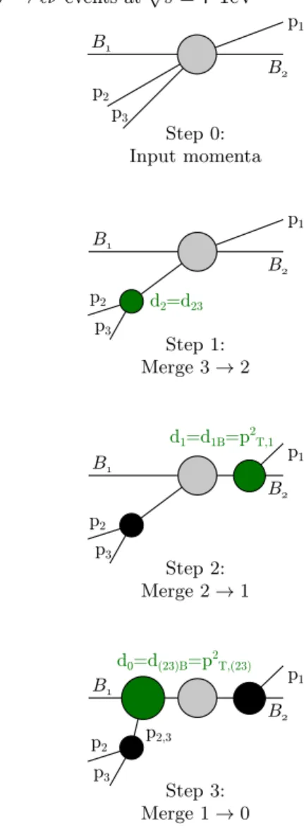
(3) 2. ATLAS: Measurement of kT splitting scales in W → `ν events at. chosen to be R = 0.6 in this paper, which is an intermediate choice between small values R ≈ 0.2, whose narrow width minimizes the impact of pileup and the underlying event, and R ≈ 1.0, whose large width efficiently collects radiation. The clustering from the set of input momenta proceeds along the following lines: 1. Calculate dij and diB for all i and j from the input momenta according to Eq. (1). 2. Find their minimum. (a) If the minimum is a dij , combine i and j into a single momentum in the list of input momenta: pij = pi + pj (b) If the minimum is a diB , remove i from the input momenta and declare it to be a jet. 3. Return to step 1 or stop when no particle remains. The observables measured are defined as the smallest p of the square roots of the dij and diB variables ( dij , √ diB ) found at each step in the clustering sequence. To simplify the notation √ they are commonly referred to as the splitting scales dk , which stand for the minima that occur when the input list proceeds from k+1 to k momenta √ by clustering and removing in each step. For example, d0 is found from the last step in the clustering sequence and reduces to the transverse momentum of the highest-pT jet. Figure 1 schematically displays the clustering sequence derived from an original input configuration of three objects labelled p1 , p2 , p3 in the presence of beams B1 and B2 . In the first clustering step, where three objects are grouped into two (denoted 3 → 2), the minimal splitting scale is found between momenta p2 and p3 , leading to d2 = d23 . In the second step (2 → 1), the momentum p1 is closest to the beam, and thus is removed and declared a jet at the scale d1 = d1B = p2T1 . Ultimately, the third clustering (1 → 0) has only the beam distance of the combined input p2,3 remaining, leading to a scale of d0 = d(23)B = p2T,(23) . 1.2 Features of the observables An important feature of these observables √ is their separation into two regions: a “hard” one with dk & 20 GeV which is dominated by perturbative QCD effects, and a “soft” one in which more phenomenological modelling aspects such as hadronisation and multiple partonic interactions may exert substantial influence on theory predictions. The number of events in the hard region for high k is naturally low in the data sample analysed for this measurement. Thus for statistical reasons values of 0 ≤ k ≤ 3 are considered in this publication. No explicit jet requirement is imposed in the event selection. In addition to the observables mentioned above, it is also interesting to study ratios of consecutive clustering p values, dk+1 /dk , where some experimental uncertainty cancellations occur, as discussed p in Sect. 6. Of particular interest is the region where dk+1 /dk → 1, as it probes events with subsequent emissions at similar scales. Those. √ s = 7 TeV. Step 0: Input momenta. Step 1: Merge 3 → 2. Step 2: Merge 2 → 1. Step 3: Merge 1 → 0 Fig. 1. Illustration of the kT clustering sequence starting from the original input configuration (three objects p1 , p2 , p3 , and beams B1 , B2 ). At each step, k + 1 objects are merged to k.. events could be challenging to describe correctly for parton shower generators without matrix element corrections. The splitting scale ratio amounts to a normalisation of the splitting scale to the scale of the QCD activity in the “underlying process”, i.e. after the clustering. To reduce the influence of non-perturbative effects, each ratio p observable d /d k+1 k is measured with events satisfying √ dk > 20 GeV. The central idea underlying this measurement is that the measure of the kT algorithm corresponds relatively well to the singularity structure of QCD. To illustrate this, the small-angle limit of the squared kT measure is given in terms of the angle θij between two momenta i and j, and the energy corresponding to the softer momentum, Ei , by [15]: 2 2 p2Ti ∆Rij ' Ei2 θij. p2Ti. '. 2 Ei2 θiB. (2) ,. (3).

(4) ATLAS: Measurement of kT splitting scales in W → `ν events at. while the splitting probability for a final-state branching into partons i and j evaluates to dPij→i,j 1 ∼ dEi dθij min(Ei , Ej )θij. (4). in the collinear limit [17]. From a comparison of Eqs. (2) and (4) it can be seen that each step of the kT algorithm identifies the parton pair which would be the most likely to have been produced by QCD interactions. In that sense, this clustering sequence mimicks the reversal of the QCD evolution. In contrast the anti-kt [18] algorithm cannot be used in the same way: its distance measure replaces all p2T by p−2 T . So even though collinear branchings are still clustered first, the same is not true for soft emissions anymore. Thus the splitting structure within the anti-kt algorithm must be constructed via the kT splitting algorithm [19]. Just like QCD matrix elements, the kT splitting scales provide a unified view of initial- and final-state radiation. Through the combination of the distance to the beams √ and the relative distance of objects to each other, the dk distributions contain information about both the pT spectra and the substructure of jets. 1.3 Existing predictions and measurements The kT splittings and related distributions have attracted the attention of theorists, in W → `ν and similar final states. They can be resummed analytically at next-toleading-logarithm accuracy as demonstrated for the example of jet production by QCD processes in hadron collisions in Refs. [20, 21]. The ratio observable y23 defined by p the authors is closely related to the ratio observables dk+1 /dk in this analysis. Other theoretical studies may be found in Refs. [22, 23]. Experimentally, these kinds of observables were measured at LEP [24–26] using the e+ e− (Durham) kT algorithm. Their theoretical features (resummability) were used in Refs. [27, 28] to determine αs with high precision. Related observables were also measured at HERA [29–32].. 2 Data analysis. √ s = 7 TeV. 3. detector covers the vertex region and typically provides three measurements per track. It is followed by the silicon microstrip tracker which usually provides four twodimensional measurement points per track. These silicon detectors are complemented by the transition radiation tracker, which contributes to track reconstruction up to |η| = 2.0. The transition radiation tracker also provides electron identification information based on the fraction of hits (typically 30 in total) above a higher energy-deposit threshold corresponding to transition radiation. The calorimeter system covers the pseudorapidity range |η| < 4.9. Within the region |η| < 3.2, electromagnetic calorimetry is provided by barrel and endcap high-granularity lead/liquid-argon (LAr) calorimeters, with an additional thin LAr presampler covering |η| < 1.8 to correct for energy loss in material upstream of the calorimeter. Hadronic calorimetry is provided by a steel/scintillatortile calorimeter, segmented radially into three barrel structures within |η| < 1.7, and two copper/LAr hadronic endcap calorimeters. The solid angle coverage is completed with forward copper/LAr and tungsten/LAr calorimeter modules optimised for electromagnetic and hadronic measurements respectively. The muon spectrometer comprises separate trigger and high-precision tracking chambers measuring the deflection of muons in a magnetic field generated by superconducting air-core toroids. The precision chamber system covers the region |η| < 2.7 with three layers of monitored drift tubes, complemented by cathode strip chambers in the forward region, where the background is highest. The muon trigger system covers the range |η| < 2.4 with resistive plate chambers in the barrel, and thin gap chambers in the endcap regions. A three-level trigger system is used to select interesting events [34]. The Level-1 trigger is implemented in hardware and uses a subset of detector information to reduce the event rate to a design value of at most 75 kHz. This is followed by two software-based trigger levels which together reduce the event rate to about 200 Hz.. 2.2 Event selection The selection of W events is based on the criteria described in Refs. [13, 35] and summarised briefly below.. 2.1 The ATLAS detector 2.2.1 Data sample and trigger The ATLAS detector [33] at the LHC covers nearly the entire solid angle around the collision point. It consists of an inner tracking detector surrounded by a thin superconducting solenoid, electromagnetic and hadronic calorimeters, and a muon spectrometer incorporating three large superconducting toroid magnets. The inner-detector system is immersed in a 2 T axial magnetic field and provides charged particle tracking in the range |η| < 2.5 1 . The high-granularity silicon pixel 1 ATLAS uses a right-handed coordinate system with its origin at the nominal interaction point (IP) in the centre of the. √ The entire 2010 data sample at s = 7 TeV was used, corresponding to an integrated luminosity of approximately 36 pb−1 . The 2010 data sample was chosen due to the low pileup conditions during data taking, where the mean detector and the z-axis along the beam pipe. The x-axis points from the IP to the centre of the LHC ring, and the y-axis points upward. Cylindrical coordinates (r, φ) are used in the transverse plane, φ being the azimuthal angle around the beam pipe. The pseudorapidity is defined in terms of the angle θ as η = − ln tan(θ/2)..

(5) 4. ATLAS: Measurement of kT splitting scales in W → `ν events at. number of interactions per bunch crossing was at most 2.3 during that period. In the W → µν analysis, the first few pb−1 were excluded to restrict to a data sample of events recorded with a uniform trigger configuration and optimal detector performance. Single-lepton triggers were used to retain W → `ν candidate events. For the electron channel a trigger threshold of 14 GeV for early data-taking periods and 15 GeV for later data-taking periods was applied. For the muon channel a trigger threshold of 13 GeV was applied. All relevant detector components were required to be fully operational during the data taking. Events with at least one reconstructed interaction vertex within 200 mm of the interaction point in the z direction and having at least three associated tracks were considered. The number of reconstructed vertices reflects the pileup conditions and, in both channels, was used to reweight the MC simulation to improve its modelling of the pileup conditions observed in data. The number of reconstructed vertices was also used to estimate the uncertainty due to possible mismodelling of the pileup. 2.2.2 Electron selection Clusters formed from energy depositions in the electromagnetic calorimeter were required to have matched tracks, with the further requirement that the cluster shapes are consistent with electromagnetic showers initiated by electrons. On top of the tight identification criteria, a calorimeter-based isolation requirement for the electron was applied to further reduce the multi-jet background. Additional requirements were applied to remove electrons falling into calorimeter regions with non-operational LAr readout. The kinematic requirements on the electron candidates included a transverse momentum requirement p`T > 20 GeV and pseudorapidity |η ` | < 2.47 with removal of the transition region 1.37 < |η ` | < 1.52 between the calorimeter modules. Exactly one of these selected electrons was required for the W → eν selection. In constructing the kT cluster sequence, clusters of calorimeter cells included in a reconstructed jet within ∆R = 0.3 of the electron candidate were removed from the input configuration. 2.2.3 Muon selection Muon candidates were required to have tracks reconstructed in both the muon spectrometer and inner detector, with p`T above 20 GeV and pseudorapidity |η ` | < 2.4. Requirements on the number of hits used to reconstruct the track in the inner detector were applied, and the muon’s point of closest approach to the primary vertex was required to be displaced in z by less than 10 mm. Trackbased isolation requirements were also imposed on the reconstructed muon. At least one muon was required for the W → µν selection. To retain consistency with the acceptance in the electron channel, when constructing the kT cluster sequence, clusters of calorimeter cells falling close to the muon candidate were removed from the input configuration as in the electron selection.. √ s = 7 TeV. 2.2.4 Selection of W candidate events and construction of observables The W → `ν event selection required that the magnimiss tude of the missing transverse momentum, ET [36], be greater than 25 GeV. The reconstructed transverse mass obtained from the lepton transverse momentum p~T` and ~ miss vectors was required to fulfil E T q ~ miss ) > 40 GeV. No requiremW = 2(p` E miss − p~ ` · E T. T. T. T. T. ments were made with respect to the number of reconstructed jets in the event. The observables defined in Sect. 1.1 were constructed using calorimeter energy clusters within a pseudorapidity range of |η cl | < 4.9. The clusters were seeded by calorimeter cells with energies at least 4σ above the noise level. The seeds were then iteratively extended by including all neighbouring cells with energies at least 2σ above the noise level. The cell clustering was finalised by the inclusion of the outer perimeter cells around the cluster. The so-called topological clusters that resulted were calibrated to the hadronic energy scale [37, 38], by applying weights to account for calorimeter non-compensation, energy lost upstream of the calorimeters and noise threshold effects. 2.3 Background treatment The contributions of electroweak backgrounds (Z → ``, W → τ ν and diboson production), as well as tt and singletop-quark production, to both channels were estimated using the MC simulation. The absolute normalisation was derived using the total theoretical cross sections and corrected using the acceptance and efficiency losses of the event selection. The shape and normalisation of the distributions of various observables for the multi-jet background were determined using data-driven methods in both analysis channels. For the W → eν selection, the background shape was obtained from data by reversing certain calorimeter-based electron identification criteria to produce a multi-jet-enriched sample. Similarly, to estimate the multi-jet contribution to W → µν, the background shape was obtained from data by inverting the requirements on the muon transverse impact parameter and its significance. These multi-jet enriched samples provided the shapes of the distributions of multi-jet background observables. The normalisation of the multi-jet background was determined by fitting a linear combinamiss tion of the multi-jet and leptonic ET shapes to the miss observed ET distribution, following the procedures described in Refs. [13, 35]. The total background was thus estimated to be 5% of the signal for the W → eν analysis, with the largest contribution arising from multi-jet production. For the W → µν analysis, the total background is 9% of the signal and is dominated by the Z → `` process. At large splitting scales, top quark pair production becomes the dominant contribution in both channels.. 3 Monte Carlo simulations All detector-level studies and the extraction of particlelevel distributions involved two signal MC generators, Alp-.

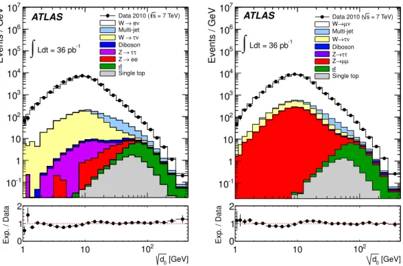
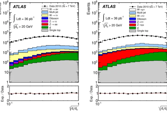
(6) ATLAS: Measurement of kT splitting scales in W → `ν events at. gen+Herwig and Sherpa. Alpgen v2.13 [39], a matrixelement (ME) generator, was interfaced to Herwig v6.510 [40] for parton showering (PS) and hadronisation, and to Jimmy v4.31 [41] for multiple parton interactions. The MLM [22] matching scheme was used to combine W boson production samples having up to five partons with the parton shower, with the matching scale set at 20 GeV. Sherpa v1.3.1 [42] was used to generate an alternative signal sample of events with W + jets, using a ME+PS merging approach [23] to prevent double counting from the parton shower, and extending the original CKKW method [43] by taking into account truncated shower emissions. Up to five partons were generated in the ME and the matching scale was set to 30 GeV. The single-top-quark background events were generated at next-to-leading-order (NLO) accuracy using the Mc@Nlo v3.3.1 [44] generator. Mc@Nlo was interfaced to Herwig and Jimmy. The Powheg v1.01 [45] generator, interfaced to Pythia6 v6.421 [46], was used to simulate the tt̄ background. The background from diboson production was generated using Herwig. Backgrounds from inclusive Z production were simulated using Pythia6. Three sets of parton density functions (PDFs) were used in these MC samples: CTEQ6L1 [47] for the Alpgen samples and the parton showering and underlying event in the Powheg samples interfaced to Pythia6; MRST 2007 LO∗ [48] for Pythia6 and Herwig; and CTEQ6.6M [49] for Mc@Nlo, Sherpa, and the NLO matrix element calculations in Powheg. The underlying event tunes were AUET1 [50] for the Herwig, Alpgen, and Mc@Nlo samples, and AMBT1 [51] for the Pythia6 and Powheg samples. The samples generated with Sherpa used the default underlying event tune. Each generated event was passed through the standard ATLAS detector simulation [52], based on Geant4 [53]. The MC events were reconstructed and analysed using the same software chain as applied to the data. The resulting MC predictions for the samples were normalised to their respective theoretical cross sections calculated at NLO [13], with the exception of the W and Z samples which were normalised to NNLO [54], and the multi-jet background which was normalised to a value extracted from the data as is described in Sect. 2. At the particle level, some additional W +jets NLO MC generators were compared to the final results. The Powheg [45,55] samples were matched to Pythia6 v6.425 or Pythia8 v8.165 [56] for parton showering and hadronisation, while another sample was generated with Mc@Nlo v4.06 [44] using Herwig v6.520.2. The Sherpa Menlops sample used Sherpa v1.4.1 with its built-in Menlops method [4], allowing an NLO+PS matched sample for inclusive W production [57] to be merged with LO matrix elements for a W boson and up to five partons using a matching scale at 20 GeV. All these NLO samples were generated with the CT10 PDF set [58]. The Mc@Nlo, Powheg and Alpgen+Herwig samples were supplemented with a simulation of QED finalstate radiation using Photos v2.15.4 [59] and tau decays using Tauola v27feb06 [60]. The Sherpa samples. √ s = 7 TeV. 5. included QED final-state radiation in a different resummation approach [61] and a built-in tau decay algorithm.. 4 Detector-level comparisons of Monte Carlo to data The √ observed and expected detector-level distributions for d0 in the electron and muon channels are shown in Fig. 2, where the MC signal predictions are provided by Alpgen+Herwig normalised to NNLO predictions [54]. The W -boson kinematic distributions are shown detail in √ in √ Refs. [13, 35]. The corresponding plots for d , d2 and 1 √ d3 can be found in Appendix A.1. Figure 3 shows the ratio of the second-hardest to the hardest splitting scale in each event. Again, the sub-leading ratio distributions at detector level are displayed √ in Appendix A.1. For the hardest clustering in the event, d0 , generally good agreement between the Alpgen+Herwig MC predictions and the data is observed. The agreement is similar for both the electron and the muon channels.. 5 Particle-level extraction 5.1 Corrections for detector effects After subtraction of backgrounds, the detector level distributions were corrected (“unfolded”) to the final-state particle level separately for the two channels, taking into account the effects of pileup and detector response. The unfolding was performed with the RooUnfold [62] package, using a Bayesian algorithm [63], in which Bayes theorem was used to derive the particle-level distributions from the detector-level distributions, over three iterations. The input for the algorithm at particle and detector level was taken from the Alpgen+Herwig sample as a default. Both the MC simulation and data-driven methods were used to demonstrate that this iterative Bayesian method was able to recover the corresponding particle-level distributions. The selection requirements applied to the event at the particle level are: • • • • •. p`T > 20 GeV (` = electron e or muon µ) |η e | < 2.47 excluding 1.37 < |η e | < 1.52 |η µ | < 2.4 pνT,lead > 25 GeV (νlead = highest-pT neutrino in event) mW T > 40 GeV. Only events with exactly one lepton passing the requirements were taken into account. Leptons were defined to include all photon radiation within a cone of ∆R = 0.1 around the final-state lepton as suggested in Ref. [64]. All lepton requirements were calculated from these combined objects. The observables defined in Sect. 1.1 were constructed using all stable particles within a pseudorapidity range of |η cl | < 4.9 with lifetime greater than 10 ps, excluding the lepton and neutrino originating from the W boson decay..

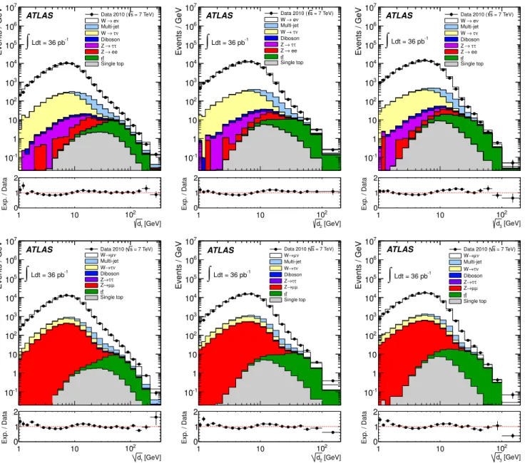
(7) Events / GeV. 107. ATLAS. 6. 10. 105. ∫ Ldt = 36 pb. -1. 104. Events / GeV. ATLAS: Measurement of kT splitting scales in W → `ν events at. 6. Data 2010 ( s = 7 TeV) W → eν Multi-jet W → τν Diboson Z → ττ Z → ee tt Single top. 107 10. 104. 102. 10. 10. 1. 1. 10-1. 10-1. 2. 2. Exp. / Data. 102. Exp. / Data. 103. 1 10. ∫ Ldt = 36 pb. -1. 105. 103. 0 1. ATLAS. 6. 102. √ s = 7 TeV Data 2010 ( s = 7 TeV) W→µν Multi-jet W→τ ν Diboson Z→τ τ Z→µµ tt Single top. 1 0. 1. 10. d0 [GeV]. 102 d0 [GeV]. √ Fig. 2. Uncorrected splitting scale d0 for events passing the W → eν (left) and W → µν (right) selection requirements. The distributions from the data (markers) are compared with the predicted signal from the MC simulation, provided by Alpgen+Herwig and normalised to the NNLO prediction. In addition, physics backgrounds, also shown, have been added in proportion to the predictions from the MC simulation. The ratio between the expectation and the data is shown in the lower plot. The error bars shown on the data are statistical only.. 5.2 Weighted combination To reduce the impact of imperfect MC modelling of pileup effects, whilst optimising the statistical power available, two different event samples were defined and utilised as follows. – “Low-pileup sample”: exactly one reconstructed vertex was required in data. The response matrices used to unfold the data and the background templates were also constructed from events where exactly one reconstructed vertex was required. – “High-pileup sample”: as above, with the difference that the number of reconstructed vertices was required to be greater than one. √ At large dk , the statistical uncertainty of the highpileup sample is smaller√than that in the low-pileup sample. However, at small dk , the systematic pileup uncertainty of the low-pileup sample is smaller than that in the high-pileup sample. To minimise the overall uncertainty on the measurement, the distributions were combined as follows. For each bin of the final distribution, the best estimate N was calculated from the bin contents N1 , N2 of the distributions in the low-pileup and high-pileup samples respectively, as N=. N1 · W1 + N2 · W2 . W1 + W2. (5). The weights Wi for each sample were constructed from the inverse of the sum in quadrature of the statistical and pileup uncertainties on the low-pileup and the high-pileup samples. The evaluation of the pileup uncertainty on each sample is described in detail in Sect. 6. The statistical uncertainty of the final distribution was calculated assuming no correlation between the two samples.. 6 Systematic uncertainties To evaluate the impact of a particular source of systematic uncertainty at the particle level, the observable considered was varied within its uncertainty, the response matrix was recalculated taking this variation into account, and the new response matrix was used to unfold the data. The fractional shift in the resulting unfolded data from nominal was interpreted as the systematic uncertainty due to that particular effect. The separate sources of uncertainty are described in the following. The relative systematic uncertainty on the energy scale of the topological clusters was evaluated from a combination of MC studies and single-pion response measurecl ments [36] to be 1 ± a × (1 + b/pcl T ) where pT represents the transverse momentum of each cluster. The constants a and b were determined to be a = 3 (10)% when |η cl | < 3.2 (|η cl | > 3.2), and b = 1.2 GeV. A shift of the cluster energy results in a shift of the distributions to higher or.

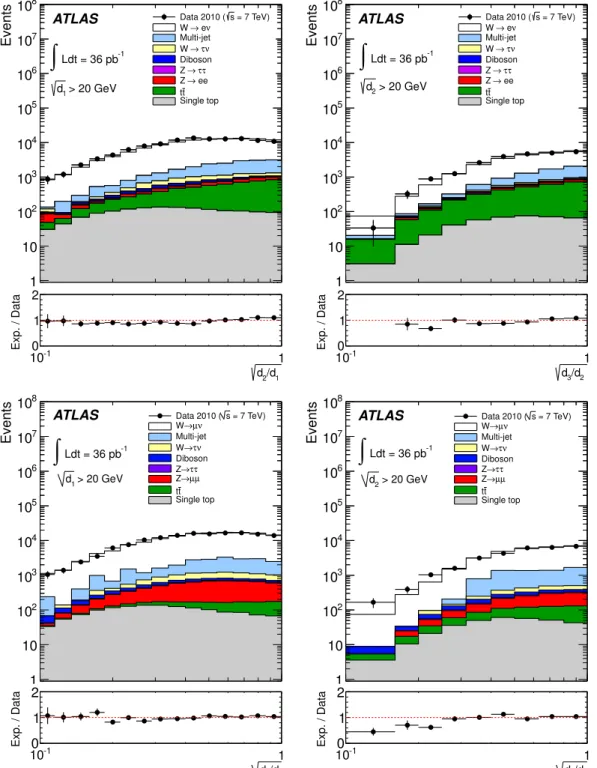
(8) ATLAS. 7. 10. 6. 10. ∫. -1. Ldt = 36 pb. d0 > 20 GeV 5. 10. Events. 108. Data 2010 ( s = 7 TeV) W → eν Multi-jet W → τν Diboson Z → ττ Z → ee tt Single top. 108 10 10. d0 > 20 GeV. 105 104. 103. 103. 102. 102. 10. 10. 1. 1 2. Exp. / Data. ∫ Ldt = 36 pb. -1. 6. 104. 2 1 0 10-1. ATLAS. 7. Exp. / Data. Events. ATLAS: Measurement of kT splitting scales in W → `ν events at. 1 d1/d0. √ s = 7 TeV. 7. Data 2010 ( s = 7 TeV) W→µν Multi-jet W→τ ν Diboson Z→τ τ Z→µµ tt Single top. 1 0. 10-1. 1 d1/d0. p Fig. 3. Uncorrected ratio d1 /d0 for events passing the W → eν (left) and W → µν (right) selection requirements. The distributions from the data (markers) are compared with the predicted signal from the MC simulation, provided by Alpgen+Herwig and normalised to the NNLO prediction. In addition, physics backgrounds, also shown, have been added in proportion to the predictions from the MC simulation. The ratio between the expectation and the data is shown in the lower plot. The error bars shown on the data are statistical only.. √ lower values. The uncertainty due to the cluster energy ting p scales dk and is largest for small splitting scales. For scale was thus evaluated separately for the low-pileup and the dk+1 /dk ratio distributions the uncertainty ranges high-pileup distributions and combined in a weighted lin- from 1% to 15%. ear sum. The uncertainty ranges from 5% to 55% p for the √ The uncertainty inherent in the unfolding procedure itsplitting scales dk and from 2% to 85% for the dk+1 /dk self was estimated by reweighting the response matrix in ratio distributions. the unfolding such that Alpgen+Herwig would accuThe lepton trigger, identification and reconstruction rately model the distribution under consideration as meaefficiencies as well as the lepton energy scale and resolution sured from data at reconstruction level. A second variawere measured in data using Z → `` events via the tagtion was performed by creating a response matrix from and-probe method, as described in Refs. [13, 35, 65]. √ The Sherpa. The larger effect, per bin, obtained from these uncertainty is less than 3% p for the splitting scales dk two estimates of the systematic uncertainty was taken as and less than 1% for the dk+1 /dk ratio distributions. the systematic uncertainty due to unfolding. The uncerThe systematic uncertainty due to possible MC mis- tainty ranges between 5% and 55% for the splitting scales √ √ modelling of pileup was evaluated separately on the lowdk , being√largest for small valuespof dk and in the pileup and high-pileup distributions. The impact of pileup vicinity of dk ≈ 15 GeV. For the dk+1 /dk ratio dismismodelling on the low-pileup sample was evaluated by tributions the uncertainty ranges between 1% and 35%. varying the requirements on the z-displacement of the The systematic uncertainties on the electroweak and interaction vertex and the number of associated tracks. An additional uncertainty accounts for the possible mis- top-quark background normalisations were assigned usmodelling of contributions from adjacent bunch-crossings. ing the theoretical uncertainty on the cross section of It was evaluated by comparing two different data-taking each process under consideration. The uncertainty on the periods: one in which proton bunches were arranged in multi-jet background normalisation was obtained by varytrains, and the other without bunch trains. The impact of ing the methods used for extracting this value from data, pileup mismodelling on the high-pileup sample was eval- as described in Refs. [13, 35]. An additional uncertainty uated as the fractional difference between the particle- was included on the shape of the multi-jet contribution, level measurements for the low-pileup and the high-pileup which was derived by comparing data-driven and simulaevents, with the statistical uncertainty subtracted in quadra- tion estimates of this background contribution. The unture. The uncertainty ranges from 1% to 30% for the split- certainty ranges from 0.5% to 15% for the splitting scales.

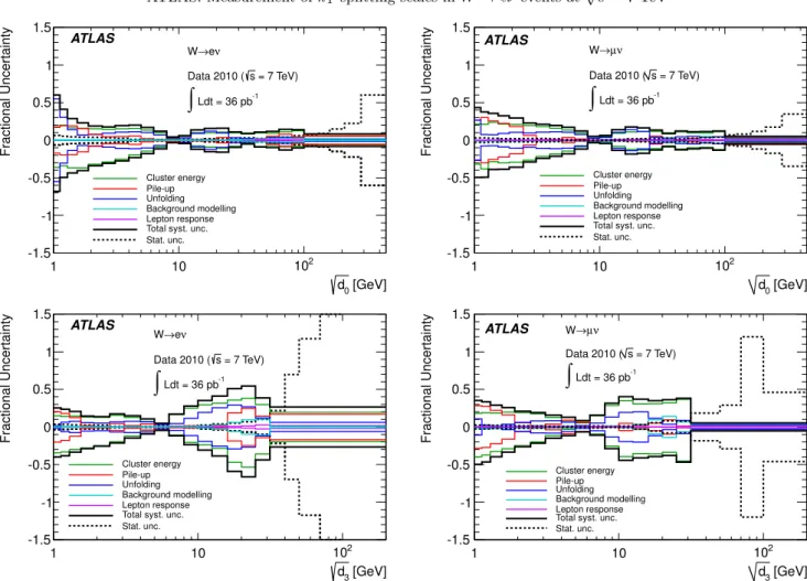
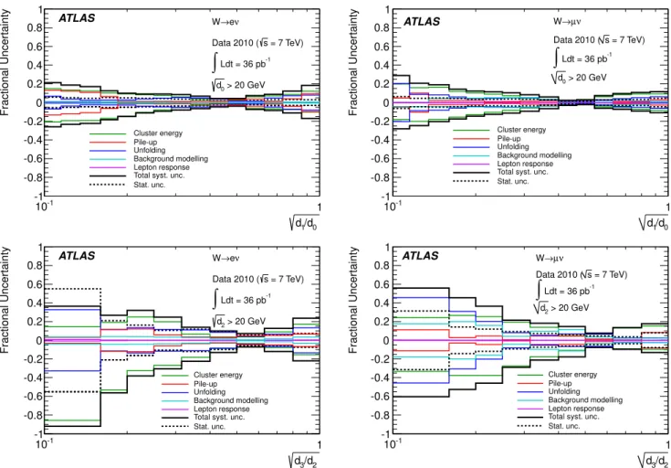
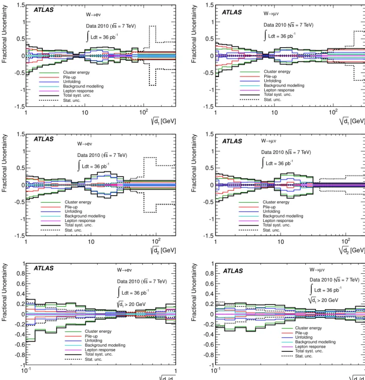
(9) Fractional Uncertainty. 1.5. Fractional Uncertainty. ATLAS: Measurement of kT splitting scales in W → `ν events at. 8 ATLAS. W→eν. 1. Data 2010 ( s = 7 TeV). ∫ Ldt = 36 pb. -1. 0.5 0 -0.5. -1.5 1. W→ µ ν Data 2010 ( s = 7 TeV). ∫ Ldt = 36 pb. -1. 0.5 0. Cluster energy Pile-up Unfolding Background modelling Lepton response Total syst. unc. Stat. unc.. -1 -1.5. 102. 10. ATLAS. 1. -0.5. Cluster energy Pile-up Unfolding Background modelling Lepton response Total syst. unc. Stat. unc.. -1. 1.5. √ s = 7 TeV. 1. 102. 10. 1.5 1. ATLAS. W→eν Data 2010 ( s = 7 TeV). ∫ Ldt = 36 pb. -1. 0.5 0 -0.5 -1 -1.5 1. 1.5 ATLAS 1. Data 2010 ( s = 7 TeV) -1. 0. -1. 102 d3 [GeV]. W→ µ ν. ∫ Ldt = 36 pb. 0.5. -0.5. Cluster energy Pile-up Unfolding Background modelling Lepton response Total syst. unc. Stat. unc.. 10. d0 [GeV] Fractional Uncertainty. Fractional Uncertainty. d0 [GeV]. Cluster energy Pile-up Unfolding Background modelling Lepton response Total syst. unc. Stat. unc.. -1.5 1. Fig. 4. Summary of the systematic uncertainties on the measured particle-level distributions for in the W → eν (left) and W → µν (right) channels.. p dk and from 1% to 20% for the dk+1 /dk ratio distributions. The magnitudes of the separate uncertainties for the hardest and fourth-hardest splittings are summarised in Figs. 4 and 5, where the statistical errors are also shown. Other cases are available in Appendix A.2. The cluster energy scale, pileup, and the unfolding procedure are the dominant sources of uncertainty in both the electron and muon channels. For each uncertainty an error band was calculated, where the upper limit is defined as the variation leading to larger values compared to the nominal distribution and the lower limit as the variation leading to lower values. To avoid underestimating the uncertainty in bins where statistical fluctuations were large, if both variations led to a shift in the same direction the larger difference with respect to the nominal distribution was taken as a symmetric uncertainty. Correlations between separate sources of systematic uncertainties and between different bins of the distributions were not considered. The quadratic sum of all systematic uncertainties considered above was taken to be the overall systematic uncertainty on the distributions. The overall systematic uncertainty ranges between 10% √ and 60% for the dk distributions, being largest for small √. 102 d3 [GeV]. 10. √. d0 (top) and. √ d3 (bottom). √ splitting scales and in the vicinity of d√ k ≈ 15 GeV. The uncertainty is smallest in the vicinity of dk ≈ 10 GeV as this corresponds to the peak of the distribution p and is thus less sensitive to scale uncertainties. For the dk+1 /dk ratio distributions the overall systematic uncertainty ranges between 5% and 95%, being largest for small values of the ratios. The statistical uncertainty on the unfolded measurement was combined in quadrature with the systematic uncertainty to obtain the total uncertainty.. 7 Results The different MC simulations in Sect. 3 were compared to the data using Rivet [66]. The FastJet library [19] was used to construct √ the kT cluster sequence. Figures 6 and 7 display the dk distributions, which have been individually normalised to unity to allow for shape comparisons. The Alpgen+Herwig MC simulation generally agrees very well with the data, as already seen in the detectorlevel distributions. The discrepancies between the MC and data distributions are covered by the systematic and statistical uncertainties. The Sherpa predictions are almost.

(10) 1. ATLAS. Fractional Uncertainty. Fractional Uncertainty. ATLAS: Measurement of kT splitting scales in W → `ν events at W→eν. 0.8. Data 2010 ( s = 7 TeV). 0.6. ∫. 0.4 0.2. -1. Ldt = 36 pb. d0 > 20 GeV. 0 -0.2 Cluster energy Pile-up Unfolding Background modelling Lepton response Total syst. unc. Stat. unc.. -0.6 -0.8. W→ µ ν. ATLAS. Data 2010 ( s = 7 TeV). 0.6. ∫ Ldt = 36 pb. -1. 0.4. d0 > 20 GeV. 0.2 0. Cluster energy Pile-up Unfolding Background modelling Lepton response Total syst. unc. Stat. unc.. -0.4 -0.6 -0.8. -1 -1 10. 9. 1 0.8. -0.2. -0.4. √ s = 7 TeV. -1 -1 10. 1. 1 d1/d0. 1 0.8 0.6. ATLAS. Fractional Uncertainty. Fractional Uncertainty. d1/d0 W→eν Data 2010 ( s = 7 TeV). 0.4. ∫ Ldt = 36 pb. 0.2. d2 > 20 GeV. -1. 0 -0.2 -0.4 -0.6 -0.8 -1 -1 10. 1. ATLAS. W→ µ ν. 0.8. Data 2010 ( s = 7 TeV). ∫ Ldt = 36 pb. 0.6. -1. 0.4. d2 > 20 GeV. 0.2 0 -0.2. Cluster energy Pile-up Unfolding Background modelling Lepton response Total syst. unc. Stat. unc.. Cluster energy Pile-up Unfolding Background modelling Lepton response Total syst. unc. Stat. unc.. -0.4 -0.6 -0.8 1. -1 -1 10. 1 d3/d2. d3/d2. Fig. 5. Summary of the systematic uncertainties on the measured particle-level ratios for in the W → eν (left) and W → µν (right) channels.. identical to those from Alpgen+Herwig in the hard re√ gion of the distributions, dk > 20 GeV, where tree-level matrix elements are applied. All three generators based on NLO+PS methods, i.e. Mc@Nlo, Powheg+Pythia6 and Powheg+Pythia8, predict significantly less hard activity than that found in data. As expected, this effect is strongest for higher multiplicities k ≥ 1, where in NLO+PS generators no matrix elements are used for the description of the QCD emission. It is interesting that they also do not √describe well the hard tail of the hardest splitting scale d0 , even though they are nominally at the same leading-order accuracy as Alpgen+Herwig and Sherpa in this distribution. This may be due to differences in higher-multiplicity parton processes becoming relevant in that region or different scale choices in the real-emission matrix element or a combination of both. In the intermediate region of 10–20 GeV, both Sherpa √ and Mc@Nlo show a similar excess over data in all dk . For Sherpa it is compensated by an undershoot in the very soft region, while for Mc@Nlo the soft region is described well. Powheg+Pythia6 and Powheg+Pythia8 also agree with data in the soft region, and their deviations from each other due to the differences in parton showering. p. d1 /d0 (top) and. p d3 /d2 (bottom). and hadronisation lie within the experimental uncertainties. √ They give identical predictions for the hard region of d0 , where both of them should be dominated by an identical real-emission matrix element. This confirms the expectation that the hard region is dominated by perturbative effects while resummation and non-perturbative effects have a large influence in the softer regions. p The distributions of the ratios dk+1 /dk are displayed in Fig. 8. These p probe the probability for a QCD emission of hardness dk+1 given a previous emission of scale √ dk . The Herwig parton shower used with both Alpgen and Mc@Nlo gives the best description of these observables. None of the ratio observables are expected to be dominated by perturbative effects, since the bulk of the events are collected near the lower threshold p √ at √ dk = 20 GeV, and dk+1 is always softer than dk . The Powheg predictions, particularly for the case where Powheg is matched to Pythia6, deviate from the data in the p ratio of the hardest and second-hardest clustering, d1 /d0 . This is the only ratio observable that directly probes the NLO+PS matching in Powheg and Mc@Nlo..

(11) ATLAS: Measurement of kT splitting scales in W → `ν events at p 1/σ dσ/d d0 [1/GeV]. 10–1 b. 10–2. b b. 10–1. b b. ATLAS. b b b. b. Data 2010 √ R s = 7 TeV –1 Ldt = 36 pb. b b b. 10–3. b. W → eν Data (Syst + stat unc.) A LPGEN +H ERWIG S HERPA (M ENLOPS ) M C @N LO P OWHEG +P YTHIA 6 P OWHEG +P YTHIA 8. b. 10–5 10–6. MC/Data 10 1. 1 p 1/σ dσ/d d1 [1/GeV]. 10–1 b. b. b. b. b b. b. b. b b. b. 10 2. b. ATLAS b. 10–2 b. b b. 10–3. b. W → eν Data (Syst + stat unc.) A LPGEN +H ERWIG S HERPA (M ENLOPS ) M C @N LO P OWHEG +P YTHIA 6 P OWHEG +P YTHIA 8. 10–4. b. 10–5 10–6 10–7. p d0 [GeV]. b b b. b b. b. b. 0.5 10 1. 1 10–1 b. b. b. b. b b. b. b. b b. b. 10 2. b. b b b b. W → µν Data (Syst + stat unc.) A LPGEN +H ERWIG S HERPA (M ENLOPS ) M C @N LO P OWHEG +P YTHIA 6 P OWHEG +P YTHIA 8 b. b. 10–7. p d0 [GeV]. ATLAS b b. 10–6 b. b b. Data 2010 √ R s = 7 TeV –1 Ldt = 36 pb b. b b b. b. 10–8. 10–8 1.5. MC/Data. MC/Data. b. 1. 10–5. b. b. 1.5. 10–4. b. b. b. 10–3. b. b. W → µν Data (Syst + stat unc.) A LPGEN +H ERWIG S HERPA (M ENLOPS ) M C @N LO P OWHEG +P YTHIA 6 P OWHEG +P YTHIA 8. 10–2. Data 2010 √ R s = 7 TeV –1 Ldt = 36 pb. Data 2010 √ R s = 7 TeV –1 Ldt = 36 pb. b. p 1/σ dσ/d d1 [1/GeV]. 0.5. b. 10–6 b. 1. ATLAS. b. b. 10–5. 1.5. b. b. b. b. b. b. 10–4. b. √ s = 7 TeV. b. 10–3. b. b b. b b. b b. b b. b. 10–2. b. b. 10–4. MC/Data. b b. b b. b b. p 1/σ dσ/d d0 [1/GeV]. 10. 1 0.5 1. 10 1. 10 2 p d1 [GeV]. 1.5 1 0.5 1. 10 1. 10 2 p d1 [GeV]. √ √ Fig. 6. Distributions of d0 (top) and d1 (bottom) in the W → eν (left) and W → µν (right) channels, shown at particle level. The data (markers) are compared to the predictions from various MC generators, and the shaded bands represent the quadrature sum of systematic and statistical uncertainties on each bin. The histograms have been normalised to unity.. 8 Conclusions. The degree of agreement between various Monte Carlo simulations with the data varies strongly for different reA first measurement of the kT cluster splitting scales in gions of the observables. The hard tails of the distributions W boson production at a hadron–hadron collider has been are significantly better described by the multi-leg generapresented. The measurement was performed using the 2010 tors Alpgen+Herwig and Sherpa, which include exact √ data sample from pp collisions at s = 7 TeV collected tree-level matrix elements, than by the NLO+PS generawith the ATLAS detector at the LHC. The data corre- tors Mc@Nlo and Powheg. This also holds true for the √ spond to approximately 36 pb−1 in both the electron and hardest clustering, d0 , even though it is formally premuon W -decay channels. dicted at the same QCD leading-order accuracy by all of Results are presented for the four hardest splitting these generators. scales in a kT cluster sequence, and ratios of these splitting scales. Backgrounds were subtracted and the results were corrected for detector effects to allow a comparison to difIn the soft regions of the splitting scales, larger variaferent generator predictions at particle level. A weighted tions between all generators become evident. The generacombination was performed to optimise the precision of tors based on the Herwig parton shower provide a good the measurement. The dominant systematic uncertainties description of the data, while the Sherpa and Powheg+ on the measurements originate from the cluster energy Pythia predictions do not reproduce the soft regions of scale, pileup and the unfolding procedure. the measurement well..

(12) 10–1. b b. b b. b. b b. b. b b. b. Data 2010 √ R s = 7 TeV –1 Ldt = 36 pb. b b b. 10–3. b. W → eν Data (Syst + stat unc.) A LPGEN +H ERWIG S HERPA (M ENLOPS ) M C @N LO P OWHEG +P YTHIA 6 P OWHEG +P YTHIA 8. 10–4. b. b. 10–5 10–6 10–7. 10–1. ATLAS b. 10–2. b. p 1/σ dσ/d d2 [1/GeV]. p 1/σ dσ/d d2 [1/GeV]. ATLAS: Measurement of kT splitting scales in W → `ν events at. b. b. ATLAS b b b. W → µν Data (Syst + stat unc.) A LPGEN +H ERWIG S HERPA (M ENLOPS ) M C @N LO P OWHEG +P YTHIA 6 P OWHEG +P YTHIA 8. b. b. 10–4 10–5. b. Data 2010 √ R s = 7 TeV –1 Ldt = 36 pb. b. 10–3. b. 11. b. 10–6 10–7. b b b. b. 10–8 MC/Data. 1.5 1 0.5 10 1. p 1/σ dσ/d d3 [1/GeV]. 1 10–1 b. b. b. b b. b. b b. b b. 10 2 p d2 [GeV]. b. ATLAS b. 10–2. Data 2010 √ R s = 7 TeV –1 Ldt = 36 pb. b b. 10–3. b. W → eν Data (Syst + stat unc.) A LPGEN +H ERWIG S HERPA (M ENLOPS ) M C @N LO P OWHEG +P YTHIA 6 P OWHEG +P YTHIA 8. 10–4. b. 10–5 10–6 10–7 10–8. b b b. b. 1.5 1 0.5. 10–1. b b. b b. ATLAS Data 2010 √ R s = 7 TeV –1 Ldt = 36 pb. b. b. W → µν Data (Syst + stat unc.) A LPGEN +H ERWIG S HERPA (M ENLOPS ) M C @N LO P OWHEG +P YTHIA 6 P OWHEG +P YTHIA 8 b. 10–6 10–7. 1.5. 1.5. MC/Data. b. b. 10–4. b. 10 2 p d3 [GeV]. b b. b. 10–8. 10 1. b. 10 2 p d2 [GeV]. b. 10–3. b. 0.5. b. 10–2. 10–9. 1. b. 10–5. 1. 10 1. 1 p 1/σ dσ/d d3 [1/GeV]. MC/Data. b. b. 10–2. 10–8. MC/Data. b. b. b b. b b. b. b. √ s = 7 TeV. b b b. b. b b. 1 0.5 1. 10 1. 10 2 p d3 [GeV]. √ √ Fig. 7. Distributions of d2 (top) and d3 (bottom) in the W → eν (left) and W → µν (right) channels, shown at particle level. The data (markers) are compared to the predictions from various MC generators, and the shaded bands represent the quadrature sum of systematic and statistical uncertainties on each bin. The histograms have been normalised to unity.. With this discriminating power the data thus test the resummation shape generated by parton showers and the extent to which the shower accuracy is preserved by the different merging and matching methods used in these Monte Carlo simulations.. 9 Acknowledgements We thank CERN for the very successful operation of the LHC, as well as the support staff from our institutions without whom ATLAS could not be operated efficiently. We acknowledge the support of ANPCyT, Argentina; YerPhI, Armenia; ARC, Australia; BMWF and FWF, Austria; ANAS, Azerbaijan; SSTC, Belarus; CNPq and FAPESP, Brazil; NSERC, NRC and CFI, Canada; CERN; CONICYT, Chile; CAS, MOST and NSFC, China; COLCIENCIAS, Colombia; MSMT CR, MPO CR and VSC. CR, Czech Republic; DNRF, DNSRC and Lundbeck Foundation, Denmark; EPLANET, ERC and NSRF, European Union; IN2P3-CNRS, CEA-DSM/IRFU, France; GNSF, Georgia; BMBF, DFG, HGF, MPG and AvH Foundation, Germany; GSRT and NSRF, Greece; ISF, MINERVA, GIF, DIP and Benoziyo Center, Israel; INFN, Italy; MEXT and JSPS, Japan; CNRST, Morocco; FOM and NWO, Netherlands; BRF and RCN, Norway; MNiSW, Poland; GRICES and FCT, Portugal; MERYS (MECTS), Romania; MES of Russia and ROSATOM, Russian Federation; JINR; MSTD, Serbia; MSSR, Slovakia; ARRS and MVZT, Slovenia; DST/NRF, South Africa; MICINN, Spain; SRC and Wallenberg Foundation, Sweden; SER, SNSF and Cantons of Bern and Geneva, Switzerland; NSC, Taiwan; TAEK, Turkey; STFC, the Royal Society and Leverhulme Trust, United Kingdom; DOE and NSF, United States of America. The crucial computing support from all WLCG partners is acknowledged gratefully, in particular from CERN.

(13) √ s = 7 TeV. p 1/σ dσ/d d1 /d0. 4. 3.5. ATLAS. Data (Syst + stat unc.) A LPGEN +H ERWIG S HERPA (M ENLOPS ) M C @N LO P OWHEG +P YTHIA 6 P OWHEG +P YTHIA 8 b. 3. 2.5 2 1.5. √ s = 7 TeV) RData 2010 ( –1 pLdt = 36 pb d0 > 20 GeV W → eν. b. b. 1.5 b b. 1. b b. b. 0. 1.5. 1.5. MC/Data. 0. 1 0.5. p 1/σ dσ/d d2 /d1. 10–1. 1 p d1 /d0. 3. 2.5 2. 1.5. ATLAS. √ s = 7 TeV) RData 2010 ( –1 pLdt = 36 pb d1 > 20 GeV W → eν b. b b b. 1 0.5 1 p d1 /d0. 3. 2. b. 1.5. MC/Data. 1.5 1 0.5 10–1. 1 p d2 /d1. 3. ATLAS. Data (Syst + stat unc.) A LPGEN +H ERWIG S HERPA (M ENLOPS ) M C @N LO P OWHEG +P YTHIA 6 P OWHEG +P YTHIA 8. √ s = 7 TeV) RData 2010 ( –1 pLdt = 36 pb d2 > 20 GeV W → eν. 1 0.5 10–1. p 1/σ dσ/d d3 /d2. MC/Data. 0. p 1/σ dσ/d d3 /d2. b b b b. 0. 1.5. b b. 0.5 b. 2. b. b. b. 2.5. b. b. 1 b. b. b. b b. b b. b. b. b. ATLAS √ s = 7 TeV) RData 2010 ( –1 pLdt = 36 pb d1 > 20 GeV W → µν. Data (Syst + stat unc.) A LPGEN +H ERWIG S HERPA (M ENLOPS ) M C @N LO P OWHEG +P YTHIA 6 P OWHEG +P YTHIA 8 b. 2.5. b. b. 0.5. b. b. 1.5 b. b. 1. b. 10–1. b. b b. b. b. 0.5. p 1/σ dσ/d d2 /d1. MC/Data. b. Data (Syst + stat unc.) A LPGEN +H ERWIG S HERPA (M ENLOPS ) M C @N LO P OWHEG +P YTHIA 6 P OWHEG +P YTHIA 8. b. b b. b. b. b b. b b. b. 0.5. 3. 2.5. b. ATLAS √ s = 7 TeV) RData 2010 ( –1 pLdt = 36 pb d0 > 20 GeV W → µν. Data (Syst + stat unc.) A LPGEN +H ERWIG S HERPA (M ENLOPS ) M C @N LO P OWHEG +P YTHIA 6 P OWHEG +P YTHIA 8 b. 3.5. b. b. 4. 2. b. b. 1. p 1/σ dσ/d d1 /d0. ATLAS: Measurement of kT splitting scales in W → `ν events at. 12. 1 p d2 /d1. 3. b. 2. 1.5 b. ATLAS √ s = 7 TeV) RData 2010 ( –1 pLdt = 36 pb d2 > 20 GeV W → µν. Data (Syst + stat unc.) A LPGEN +H ERWIG S HERPA (M ENLOPS ) M C @N LO P OWHEG +P YTHIA 6 P OWHEG +P YTHIA 8 b. 2.5. b b. b. b b. b. 1. b b. 1 b. b. b. 0.5. 0.5. b b. b b. 0. 1.5. MC/Data. MC/Data. 0 b. 1 0.5 10–1. 1 p d3 /d2. 1.5 1 0.5 10–1. 1 p d3 /d2. p Fig. 8. Distributions of the dk+1 /dk ratio distributions for W → eν (left) and W → µν (right) in the data after correcting to particle level (marker) in comparison with various MC generators as described in the text. The shaded bands represent the quadrature sum of systematic and statistical uncertainties on each bin. The histograms have been normalised to unity..

(14) ATLAS: Measurement of kT splitting scales in W → `ν events at. and the ATLAS Tier-1 facilities at TRIUMF (Canada), NDGF (Denmark, Norway, Sweden), CC-IN2P3 (France), KIT/GridKA (Germany), INFN-CNAF (Italy), NL-T1 (Netherlands), PIC (Spain), ASGC (Taiwan), RAL (UK) and BNL (USA) and in the Tier-2 facilities worldwide.. √ s = 7 TeV. 13.

(15) 14. ATLAS: Measurement of kT splitting scales in W → `ν events at. References 1. C. Berger et al., Phys. Rev. Lett. 106, 092001 (2011), arXiv:1009.2338 [hep-ph]. 2. R. K. Ellis et al., J. High Energy Phys. 0901, 012 (2009), arXiv:0810.2762 [hep-ph]. 3. R. Frederix et al., J. High Energy Phys. 1202, 048 (2012), arXiv:1110.5502 [hep-ph]. 4. S. Höche et al., J. High Energy Phys. 1108, 123 (2011), arXiv:1009.1127 [hep-ph]. 5. S. Höche et al., Phys. Rev. Lett. 110, 052001 (2013), arXiv:1201.5882 [hep-ph]. 6. CDF Collaboration, T. Aaltonen et al., Phys. Rev. D 77, 011108 (2008), arXiv:0711.4044 [hep-ex]. 7. D0 Collaboration, V. M. Abazov et al., Phys. Lett. B 705, 200–207(2011), arXiv:1106.1457 [hep-ex]. 8. CMS Collaboration, Phys. Rev. Lett. 107, 021802 (2011), arXiv:1104.3829 [hep-ex]. 9. CMS Collaboration, J. High Energy Phys. 1201, 010 (2012), arXiv:1110.3226 [hep-ex]. 10. CMS Collaboration, Phys. Rev. Lett. 109, 251801 (2012), arXiv:1208.3477 [hep-ex]. 11. ATLAS Collaboration, Phys. Lett. B 708, 221–240(2012), arXiv:1108.4908 [hep-ex]. 12. ATLAS Collaboration, Phys. Lett. B 707, 418–437(2012), arXiv:1109.1470 [hep-ex]. 13. ATLAS Collaboration, Phys. Rev. D 85, 092002 (2012), arXiv:1201.1276 [hep-ex]. 14. ATLAS Collaboration, Eur. Phys. J. C 72, 2001 (2012), arXiv:1203.2165 [hep-ex]. 15. S. Catani et al., Nucl. Phys. B 406, 187 (1993). 16. S. D. Ellis and D. E. Soper, Phys. Rev. D 48, 3160–3166(1993), arXiv:hep-ph/9305266. 17. G. P. Salam, Eur. Phys. J. C 67, 637 (2010), arXiv:0906.1833 [hep-ph]. 18. M. Cacciari et al., J. High Energy Phys. 0804, 063 (2008), arXiv:0802.1189 [hep-ph]. 19. M. Cacciari et al., Eur. Phys. J. C 72, 1896 (2012), arXiv:1111.6097 [hep-ph]. 20. A. Banfi et al., J. High Energy Phys. 0408, 062 (2004), arXiv:hep-ph/0407287. 21. A. Banfi et al., J. High Energy Phys. 1006, 038 (2010), arXiv:1001.4082 [hep-ph]. 22. J. Alwall et al., Eur. Phys. J. C 53, 473 (2008), arXiv:0706.2569 [hep-ph]. 23. S. Höche et al., J. High Energy Phys. 0905, 053 (2009), arXiv:0903.1219 [hep-ph]. 24. DELPHI Collaboration, P. Abreu et al., Z. Phys. C 73, 11 (1996). 25. JADE collaboration, OPAL Collaboration, P. Pfeifenschneider et al., Eur. Phys. J. C 17, 19 (2000), arXiv:hep-ex/0001055 [hep-ex]. 26. ALEPH Collaboration, A. Heister et al., Eur. Phys. J. C 35, 457 (2004). 27. G. Dissertori et al., J. High Energy Phys. 0908, 036 (2009), arXiv:0906.3436 [hep-ph]. 28. R. Frederix et al., J. High Energy Phys. 1011, 050 (2010), arXiv:1008.5313 [hep-ph]. 29. H1 Collaboration, C. Adloff et al., Nucl. Phys. B 545, 3 (1999), arXiv:hep-ex/9901010. 30. H1 Collaboration, N. Tobien, Nucl. Phys. Proc. Suppl. 79, 469 (1999).. √ s = 7 TeV. 31. ZEUS Collaboration, S. Chekanov et al., Phys. Lett. B 558, 41 (2003), arXiv:hep-ex/0212030. 32. ZEUS Collaboration, S. Chekanov et al., Nucl. Phys. B 700, 3 (2004), arXiv:hep-ex/0405065. 33. ATLAS Collaboration, J. Instrum. 3, S08003 (2008). 34. ATLAS Collaboration, Eur. Phys. J. C 72, 1849 (2012), arXiv:1110.1530 [hep-ex]. 35. ATLAS Collaboration, Phys. Rev. D 85, 072004 (2012), arXiv:1109.5141 [hep-ex]. 36. ATLAS Collaboration, Eur. Phys. J. C 72, 1844 (2012), arXiv:1108.5602 [hep-ex]. 37. C. Issever et al., Nucl. Instrum. Methods A 545, 803 (2005), arXiv:physics/0408129 [physics]. 38. T. Barillari et al., ATL-LARG-PUB-2009-001-2 (2008). https://cds.cern.ch/record/1112035. 39. M. L. Mangano et al., J. High Energy Phys. 0307, 001 (2003), arXiv:hep-ph/0206293. 40. G. Corcella et al., J. High Energy Phys. 0101, 010 (2001), arXiv:hep-ph/0011363. 41. J. Butterworth et al., Z. Phys. C 72, 637 (1996), arXiv:hep-ph/9601371. 42. T. Gleisberg et al., J. High Energy Phys. 0902, 007 (2009), arXiv:0811.4622 [hep-ph]. 43. S. Catani et al., J. High Energy Phys. 0111, 063 (2001), arXiv:hep-ph/0109231. 44. S. Frixione and B. R. Webber, J. High Energy Phys. 0206, 029 (2002), arXiv:hep-ph/0204244. 45. S. Frixione et al., J. High Energy Phys. 0711, 070 (2007), arXiv:0709.2092 [hep-ph]. 46. T. Sjostrand et al., J. High Energy Phys. 0605, 026 (2006), arXiv:hep-ph/0603175. 47. J. Pumplin et al., J. High Energy Phys. 0207, 012 (2002), arXiv:hep-ph/0201195. 48. A. Sherstnev and R. Thorne, Eur. Phys. J. C 55, 553 (2008), arXiv:0711.2473 [hep-ph]. 49. P. M. Nadolsky et al., Phys. Rev. D 78, 013004 (2008), arXiv:0802.0007 [hep-ph]. 50. ATLAS Collaboration, ATL-PHYS-PUB-2010-014 (2010). http://cds.cern.ch/record/1303025. 51. ATLAS Collaboration, ATLAS-CONF-2010-031 (2010). http://cds.cern.ch/record/1277665. 52. ATLAS Collaboration, Eur. Phys. J. C 70, 823 (2010), arXiv:1005.4568 [physics.ins-det]. 53. GEANT4 Collaboration, S. Agostinelli et al., Nucl. Instrum. Methods A 506, 250 (2003). 54. K. Melnikov and F. Petriello, Phys. Rev. D 74, 114017 (2006), arXiv:hep-ph/0609070. 55. S. Alioli et al., J. High Energy Phys. 0807, 060 (2008), arXiv:0805.4802 [hep-ph]. 56. T. Sjostrand et al., Comput. Phys. Commun. 178, 852–867(2008), arXiv:0710.3820 [hep-ph]. 57. S. Höche et al., JHEP 1209, 049 (2011), arXiv:1111.1220 [hep-ph]. 58. H.-L. Lai et al., Phys. Rev. D 82, 074024 (2010), arXiv:1007.2241 [hep-ph]. 59. P. Golonka and Z. Was, Eur. Phys. J. C 45, 97 (2006), arXiv:hep-ph/0506026. 60. S. Jadach et al., Comput. Phys. Commun. 64, 275 (1990). 61. M. Schönherr and F. Krauss, J. High Energy Phys. 0812, 018 (2008), arXiv:0810.5071 [hep-ph]. 62. T. Adye, arXiv:1105.1160 [physics.data-an]. 63. G. D’Agostini, Nucl. Instrum. Methods A 362, 487 (1995)..

(16) ATLAS: Measurement of kT splitting scales in W → `ν events at 64. J. Butterworth et al., arXiv:1003.1643 [hep-ph]. 65. ATLAS Collaboration, Eur. Phys. J. C 72, 1909 (2012), arXiv:1110.3174 [hep-ex]. 66. A. Buckley et al., arXiv:1003.0694 [hep-ph].. √ s = 7 TeV. 15.

(17) ATLAS: Measurement of kT splitting scales in W → `ν events at. 16. √ s = 7 TeV. A Appendices. ATLAS. Data 2010 ( s = 7 TeV) W → eν Multi-jet W → τν Diboson Z → ττ Z → ee tt Single top. 106 105. ∫ Ldt = 36 pb. -1. 104. 107. Data 2010 ( s = 7 TeV) W → eν Multi-jet W → τν Diboson Z → ττ Z → ee tt Single top. ATLAS. 106 105. ∫ Ldt = 36 pb. -1. 104. 107. 105. 103. 102. 102. 102. 10. 10. 10. 1. 1. 1. -1. -1. 10-1. 2. 2. Exp. / Data. 10. 102. 0 1. 102. 10. 107 ATLAS. Data 2010 ( s = 7 TeV) W→µν Multi-jet W→τ ν Diboson Z→τ τ Z→µµ tt Single top. 106. ∫ Ldt = 36 pb. -1. 105 104. 0 1. 107 ATLAS. Data 2010 ( s = 7 TeV) W→µ ν Multi-jet W→τν Diboson Z→ττ Z→µ µ. 106. ∫ Ldt = 36 pb. -1. 105. tt Single top. 104. 107. 105. 102. 102. 10. 10. 10. 1. 1. 1. -1. -1. 10-1. 2. 2. 1. 10. 102. 1 0. 1. d1 [GeV]. Exp. / Data. Exp. / Data. Exp. / Data. 10. 10. 102 d2 [GeV]. 102. Data 2010 ( s = 7 TeV) W→µν Multi-jet W→τ ν Diboson Z→τ τ Z→µµ tt Single top. ∫ Ldt = 36 pb. -1. 104. 102. 0. ATLAS. 106. 103. 1. 10. d3 [GeV]. 103. 2. -1. 1. 103. 10. ∫ Ldt = 36 pb. d2 [GeV]. Events / GeV. d1 [GeV]. Events / GeV. Exp. / Data. 0 1. 1. Exp. / Data. 10. 1. Data 2010 ( s = 7 TeV) W → eν Multi-jet W → τν Diboson Z → ττ Z → ee tt Single top. 104. 103. 2. ATLAS. 106. 103. 10. Events / GeV. Events / GeV. 107. Events / GeV. Events / GeV. A.1 Additional detector-level comparisons. 1 0. 1. 10. 102 d3 [GeV]. √ √ √ Fig. 9. Uncorrected splitting scales d1 (left), d2 (middle) and d3 (right) for events passing the W → eν (top) and W → µν (bottom) selection requirements. The distributions from the data (markers) are compared with the predicted signal from the MC simulation, provided by Alpgen+Herwig and normalised to the NNLO prediction. In addition, physics backgrounds, also shown, have been added in proportion to the predictions from the MC simulation. The ratio between the expectation and the data is shown in the lower plot. The error bars shown on the data are statistical only..

(18) 108. ATLAS. 7. 10. 6. 10. ∫. -1. Ldt = 36 pb. d1 > 20 GeV 5. 10. Events. Events. ATLAS: Measurement of kT splitting scales in W → `ν events at Data 2010 ( s = 7 TeV) W → eν Multi-jet W → τν Diboson Z → ττ Z → ee tt Single top. 108 10 10. d2 > 20 GeV. 5. 10. 103. 103. 102. 102. 10. 10. 1. 1. 2. 2. Exp. / Data. 104. Exp. / Data. ∫ Ldt = 36 pb. -1. 6. 104. 1 0 10-1. ATLAS. 7. 1. 6. 10. ∫. -1. Ldt = 36 pb. d1 > 20 GeV. 105. Events. 10. ATLAS. 0 10-1. 108 7. 10. 1. 10. 105. 103. 103. 102. 102. 10. 10. 1 2. 1 2. Exp. / Data. 104. 0. 1 d2/d1. ∫ Ldt = 36 pb. d2 > 20 GeV. 104. 10-1. ATLAS -1. 6. 1. Data 2010 ( s = 7 TeV) W → eν Multi-jet W → τν Diboson Z → ττ Z → ee tt Single top. d3/d2. Exp. / Data. Events. 7. Data 2010 ( s = 7 TeV) W→µν Multi-jet W→τ ν Diboson Z→τ τ Z→µµ tt Single top. 17. 1. d2/d1. 108. √ s = 7 TeV. Data 2010 ( s = 7 TeV) W→µν Multi-jet W→τ ν Diboson Z→τ τ Z→µµ tt Single top. 1 0. 10-1. 1 d3/d2. p p Fig. 10. Uncorrected ratios d2 /d1 (left) and d3 /d2 (right) for events passing the W → eν (top) and W → µν (bottom) selection requirements. The distributions from the data (markers) are compared with the predicted signal from the MC simulation, provided by Alpgen+Herwig and normalised to the NNLO prediction. In addition, physics backgrounds, also shown, have been added in proportion to the predictions from the MC simulation. The ratio between the expectation and the data is shown in the lower plot. The error bars shown on the data are statistical only..

(19) ATLAS: Measurement of kT splitting scales in W → `ν events at. 18. √ s = 7 TeV. 1.5. ATLAS. 1. Fractional Uncertainty. Fractional Uncertainty. A.2 Additional summaries of systematic uncertainties. W→eν Data 2010 ( s = 7 TeV). ∫ Ldt = 36 pb. -1. 0.5 0 -0.5. -1.5 1. ATLAS 1. ∫ Ldt = 36 pb. -1. 0.5 0. Cluster energy Pile-up Unfolding Background modelling Lepton response Total syst. unc. Stat. unc.. -1 -1.5. 102. 10. W→ µ ν Data 2010 ( s = 7 TeV). -0.5. Cluster energy Pile-up Unfolding Background modelling Lepton response Total syst. unc. Stat. unc.. -1. 1.5. 1. 102. 10. ATLAS. 1. W→eν Data 2010 ( s = 7 TeV). ∫ Ldt = 36 pb. -1. 0.5 0 -0.5. -1.5 1. 1 0.8 0.6. W→eν Data 2010 ( s = 7 TeV). ∫ Ldt = 36 pb. 0.2. d1 > 20 GeV. -1. 0 -0.2 -0.6 -0.8 -1 -1 10. 1. W→ µ ν Data 2010 ( s = 7 TeV). ∫ Ldt = 36 pb. -1. 0.5 0. Cluster energy Pile-up Unfolding Background modelling Lepton response Total syst. unc. Stat. unc.. -1.5. 102 d2 [GeV]. 0.4. -0.4. ATLAS. -1. 10. ATLAS. 1.5. -0.5. Cluster energy Pile-up Unfolding Background modelling Lepton response Total syst. unc. Stat. unc.. -1. Fractional Uncertainty. Fractional Uncertainty. 1.5. d1 [GeV]. 1. Fractional Uncertainty. Fractional Uncertainty. d1 [GeV]. 1 0.8. Data 2010 ( s = 7 TeV). 0.6. ∫ Ldt = 36 pb. -1. 0.4. d1 > 20 GeV. 0.2 0 -0.4 -0.6 -0.8. 1. W→ µ ν. ATLAS. -0.2 Cluster energy Pile-up Unfolding Background modelling Lepton response Total syst. unc. Stat. unc.. 102 d2 [GeV]. 10. Cluster energy Pile-up Unfolding Background modelling Lepton response Total syst. unc. Stat. unc.. -1 -1 10. 1 d2/d1. d2/d1. Fig. 11. Summary of the systematic uncertainties on the measured particle-level distributions for p and the ratio d2 /d1 (bottom) in the W → eν (left) and W → µν (right) channels.. √. d1 (top) and. √ d2 (middle).

(20) ATLAS: Measurement of kT splitting scales in W → `ν events at. √ s = 7 TeV. 19. The ATLAS Collaboration G. Aad48 , T. Abajyan21 , B. Abbott111 , J. Abdallah12 , S. Abdel Khalek115 , A.A. Abdelalim49 , O. Abdinov11 , R. Aben105 , B. Abi112 , M. Abolins88 , O.S. AbouZeid158 , H. Abramowicz153 , H. Abreu136 , B.S. Acharya164a,164b,a , L. Adamczyk38 , D.L. Adams25 , T.N. Addy56 , J. Adelman176 , S. Adomeit98 , P. Adragna75 , T. Adye129 , S. Aefsky23 , J.A. Aguilar-Saavedra124b,b , M. Agustoni17 , S.P. Ahlen22 , F. Ahles48 , A. Ahmad148 , M. Ahsan41 , G. Aielli133a,133b , T.P.A. Åkesson79 , G. Akimoto155 , A.V. Akimov94 , M.A. Alam76 , J. Albert169 , S. Albrand55 , M. Aleksa30 , I.N. Aleksandrov64 , F. Alessandria89a , C. Alexa26a , G. Alexander153 , G. Alexandre49 , T. Alexopoulos10 , M. Alhroob164a,164c , M. Aliev16 , G. Alimonti89a , J. Alison120 , B.M.M. Allbrooke18 , L.J. Allison71 , P.P. Allport73 , S.E. Allwood-Spiers53 , J. Almond82 , A. Aloisio102a,102b , R. Alon172 , A. Alonso36 , F. Alonso70 , A. Altheimer35 , B. Alvarez Gonzalez88 , M.G. Alviggi102a,102b , K. Amako65 , C. Amelung23 , V.V. Ammosov128,∗ , S.P. Amor Dos Santos124a , A. Amorim124a,c , S. Amoroso48 , N. Amram153 , C. Anastopoulos30 , L.S. Ancu17 , N. Andari115 , T. Andeen35 , C.F. Anders58b , G. Anders58a , K.J. Anderson31 , A. Andreazza89a,89b , V. Andrei58a , X.S. Anduaga70 , S. Angelidakis9 , P. Anger44 , A. Angerami35 , F. Anghinolfi30 , A. Anisenkov107 , N. Anjos124a , A. Annovi47 , A. Antonaki9 , M. Antonelli47 , A. Antonov96 , J. Antos144b , F. Anulli132a , M. Aoki101 , L. Aperio Bella5 , R. Apolle118,d , G. Arabidze88 , I. Aracena143 , Y. Arai65 , A.T.H. Arce45 , S. Arfaoui148 , J-F. Arguin93 , S. Argyropoulos42 , E. Arik19a,∗ , M. Arik19a , A.J. Armbruster87 , O. Arnaez81 , V. Arnal80 , A. Artamonov95 , G. Artoni132a,132b , D. Arutinov21 , S. Asai155 , S. Ask28 , B. Åsman146a,146b , L. Asquith6 , K. Assamagan25,e , R. Astalos144a , A. Astbury169 , M. Atkinson165 , B. Auerbach6 , E. Auge115 , K. Augsten126 , M. Aurousseau145a , G. Avolio30 , D. Axen168 , G. Azuelos93,f , Y. Azuma155 , M.A. Baak30 , G. Baccaglioni89a , C. Bacci134a,134b , A.M. Bach15 , H. Bachacou136 , K. Bachas154 , M. Backes49 , M. Backhaus21 , J. Backus Mayes143 , E. Badescu26a , P. Bagnaia132a,132b , Y. Bai33a , D.C. Bailey158 , T. Bain35 , J.T. Baines129 , O.K. Baker176 , S. Baker77 , P. Balek127 , F. Balli136 , E. Banas39 , P. Banerjee93 , Sw. Banerjee173 , D. Banfi30 , A. Bangert150 , V. Bansal169 , H.S. Bansil18 , L. Barak172 , S.P. Baranov94 , T. Barber48 , E.L. Barberio86 , D. Barberis50a,50b , M. Barbero83 , D.Y. Bardin64 , T. Barillari99 , M. Barisonzi175 , T. Barklow143 , N. Barlow28 , B.M. Barnett129 , R.M. Barnett15 , A. Baroncelli134a , G. Barone49 , A.J. Barr118 , F. Barreiro80 , J. Barreiro Guimarães da Costa57 , R. Bartoldus143 , A.E. Barton71 , V. Bartsch149 , A. Basye165 , R.L. Bates53 , L. Batkova144a , J.R. Batley28 , A. Battaglia17 , M. Battistin30 , F. Bauer136 , H.S. Bawa143,g , S. Beale98 , T. Beau78 , P.H. Beauchemin161 , R. Beccherle50a , P. Bechtle21 , H.P. Beck17 , K. Becker175 , S. Becker98 , M. Beckingham138 , K.H. Becks175 , A.J. Beddall19c , A. Beddall19c , S. Bedikian176 , V.A. Bednyakov64 , C.P. Bee83 , L.J. Beemster105 , T.A. Beermann175 , M. Begel25 , S. Behar Harpaz152 , C. Belanger-Champagne85 , P.J. Bell49 , W.H. Bell49 , G. Bella153 , L. Bellagamba20a , M. Bellomo30 , A. Belloni57 , O. Beloborodova107,h , K. Belotskiy96 , O. Beltramello30 , O. Benary153 , D. Benchekroun135a , K. Bendtz146a,146b , N. Benekos165 , Y. Benhammou153 , E. Benhar Noccioli49 , J.A. Benitez Garcia159b , D.P. Benjamin45 , M. Benoit115 , J.R. Bensinger23 , K. Benslama130 , S. Bentvelsen105 , D. Berge30 , E. Bergeaas Kuutmann42 , N. Berger5 , F. Berghaus169 , E. Berglund105 , J. Beringer15 , P. Bernat77 , R. Bernhard48 , C. Bernius25 , F.U. Bernlochner169 , T. Berry76 , C. Bertella83 , A. Bertin20a,20b , F. Bertolucci122a,122b , M.I. Besana89a,89b , G.J. Besjes104 , N. Besson136 , S. Bethke99 , W. Bhimji46 , R.M. Bianchi30 , L. Bianchini23 , M. Bianco72a,72b , O. Biebel98 , S.P. Bieniek77 , K. Bierwagen54 , J. Biesiada15 , M. Biglietti134a , H. Bilokon47 , M. Bindi20a,20b , S. Binet115 , A. Bingul19c , C. Bini132a,132b , C. Biscarat178 , B. Bittner99 , C.W. Black150 , J.E. Black143 , K.M. Black22 , R.E. Blair6 , J.-B. Blanchard136 , T. Blazek144a , I. Bloch42 , C. Blocker23 , J. Blocki39 , W. Blum81 , U. Blumenschein54 , G.J. Bobbink105 , V.S. Bobrovnikov107 , S.S. Bocchetta79 , A. Bocci45 , C.R. Boddy118 , M. Boehler48 , J. Boek175 , T.T. Boek175 , N. Boelaert36 , J.A. Bogaerts30 , A. Bogdanchikov107 , A. Bogouch90,∗ , C. Bohm146a , J. Bohm125 , V. Boisvert76 , T. Bold38 , V. Boldea26a , N.M. Bolnet136 , M. Bomben78 , M. Bona75 , M. Boonekamp136 , S. Bordoni78 , C. Borer17 , A. Borisov128 , G. Borissov71 , I. Borjanovic13a , M. Borri82 , S. Borroni42 , J. Bortfeldt98 , V. Bortolotto134a,134b , K. Bos105 , D. Boscherini20a , M. Bosman12 , H. Boterenbrood105 , J. Bouchami93 , J. Boudreau123 , E.V. Bouhova-Thacker71 , D. Boumediene34 , C. Bourdarios115 , N. Bousson83 , S. Boutouil135d , A. Boveia31 , J. Boyd30 , I.R. Boyko64 , I. Bozovic-Jelisavcic13b , J. Bracinik18 , P. Branchini134a , A. Brandt8 , G. Brandt118 , O. Brandt54 , U. Bratzler156 , B. Brau84 , J.E. Brau114 , H.M. Braun175,∗ , S.F. Brazzale164a,164c , B. Brelier158 , J. Bremer30 , K. Brendlinger120 , R. Brenner166 , S. Bressler172 , T.M. Bristow145b , D. Britton53 , F.M. Brochu28 , I. Brock21 , R. Brock88 , F. Broggi89a , C. Bromberg88 , J. Bronner99 , G. Brooijmans35 , T. Brooks76 , W.K. Brooks32b , G. Brown82 , P.A. Bruckman de Renstrom39 , D. Bruncko144b , R. Bruneliere48 , S. Brunet60 , A. Bruni20a , G. Bruni20a , M. Bruschi20a , L. Bryngemark79 , T. Buanes14 , Q. Buat55 , F. Bucci49 , J. Buchanan118 , P. Buchholz141 , R.M. Buckingham118 , A.G. Buckley46 , S.I. Buda26a , I.A. Budagov64 , B. Budick108 , L. Bugge117 , O. Bulekov96 , A.C. Bundock73 , M. Bunse43 , T. Buran117 , H. Burckhart30 , S. Burdin73 , T. Burgess14 , S. Burke129 , E. Busato34 , V. Büscher81 , P. Bussey53 , C.P. Buszello166 , B. Butler143 , J.M. Butler22 , C.M. Buttar53 , J.M. Butterworth77 , W. Buttinger28 , M. Byszewski30 , S. Cabrera Urbán167 , D. Caforio20a,20b , O. Cakir4a , P. Calafiura15 , G. Calderini78 , P. Calfayan98 , R. Calkins106 , L.P. Caloba24a , R. Caloi132a,132b , D. Calvet34 , S. Calvet34 , R. Camacho Toro34 , P. Camarri133a,133b , D. Cameron117 , L.M. Caminada15 , R. Caminal Armadans12 , S. Campana30 , M. Campanelli77 , V. Canale102a,102b , F. Canelli31 , A. Canepa159a , J. Cantero80 , R. Cantrill76 , T. Cao40 , M.D.M. Capeans Garrido30 , I. Caprini26a , M. Caprini26a , D. Capriotti99 , M. Capua37a,37b , R. Caputo81 , R. Cardarelli133a , T. Carli30 , G. Carlino102a , L. Carminati89a,89b , S. Caron104 ,.