Impact of water in the degradability and hemocompatibility of polymers for medical applications

Texto completo

(1)PONTIFICIA UNIVERSIDAD CATOLICA DE CHILE ESCUELA DE INGENIERIA. IMPACT OF WATER IN THE DEGRADABILITY AND HEMOCOMPATIBILITY OF POLYMERS FOR MEDICAL APPLICATIONS. MIN A BAG. Thesis submitted to the Office of Research and Graduate Studies in partial fulfillment of the requirements for the Degree of Master of Science in Engineering Advisor: LORETO M. VALENZUELA. Santiago de Chile, (July, 2017)  2017, Min A Bag.

(2) PONTIFICIA UNIVERSIDAD CATOLICA DE CHILE ESCUELA DE INGENIERIA. IMPACT OF WATER IN THE DEGRADABILITY AND HEMOCOMPATIBILITY OF POLYMERS FOR MEDICAL APPLICATIONS. MIN A BAG. Members of the Committee: LORETO M. VALENZUELA DIEGO CELENTANO JAVIER ENRIONE ALFONSO CRUZ. Thesis submitted to the Office of Research and Graduate Studies in partial fulfillment of the requirements for the Degree of Master of Science in Engineering Santiago de Chile, July, 2017.

(3) “Only those who will risk going too far can possibly find out how far one can go.” – T.S. Elliot. ii.

(4) ACKNOWLEDGMENTS Foremost, I would like to express my deepest appreciation to my advisor Dr. Loreto Valenzuela, for her great patience, constant support and motivation throughout the development of this thesis. Without her guidance, this thesis would not have been possible.. I want to thank Dr. Sanjeeva Murthy from the New Jersey Center for Biomaterials for kindly providing polymer data, which was crucial for the development of this thesis.. I would like to thank Daniela Soto, who provided me with relevant information and guidance in the initial stage of this thesis. I also want to thank all the members of the Biomaterials and Biopolymers Laboratory for their support, especially to Phammela Abarzua, Valentina Frenkel, Tamara Akentjew and Raimundo Gillet, whose feedback and encouragement were deeply valued.. Finally, I must express my very profound gratitude to my parents and my sister for providing me with unfailing support and continuous encouragement throughout my entire education and the development of this thesis. Nothing of what I have accomplished would have been possible without them.. iii.

(5) GENERAL INDEX Pág. ACKNOWLEDGMENTS .......................................................................................... iii TABLE INDEX .......................................................................................................... vi FIGURE INDEX ........................................................................................................ vii NOMENCLATURE ..................................................................................................... x RESUMEN................................................................................................................ xiv ABSTRACT ............................................................................................................... xv 1.. INTRODUCTION .............................................................................................. 1 1.1. General aspects of water ............................................................................ 1 1.2. Water in biological systems ....................................................................... 3. 1.3.. 1.4. 1.5. 1.6. 2.. 1.2.1. Biochemical reactions and body function........................................ 3 1.2.2. Swelling of Medical devices ............................................................ 3 1.2.3. Polymer degradation ........................................................................ 4 Surface water .............................................................................................. 5 1.3.1. States of water................................................................................. 6 1.3.2. Water measurement techniques ...................................................... 9 Biocompatibility....................................................................................... 16 Hypothesis and Objectives ....................................................................... 18 Organization of the Document ................................................................. 19. MATHEMATICAL MODEL OF POLYMER DEGRADATION AND WATER UPTAKE........................................................................................................... 20 2.3. Model Formulation................................................................................... 21 2.3.1. Initial conditions ............................................................................ 23 2.3.2. Boundary conditions ...................................................................... 23 2.4. Simulation ................................................................................................ 24 2.4.2. Parameter estimation ..................................................................... 24 2.4.3. Species distribution evolution in polymer matrix .......................... 27 2.5. Conclusions .............................................................................................. 30.

(6) 3.. EFFECT OF WATER ON HEMOCOMPATIBILITY OF POLYMERS ....... 31 3.1. Study Selection and Data Analysis .......................................................... 31 3.2. Results on the effect of the states of water on hemocompatibility .......... 31 3.2.1. Degradable polymers .................................................................... 32 3.2.2. Non-degradable polymers .............................................................. 49 3.3. Discussion ................................................................................................ 55 3.3.1. Water states in polymers ................................................................ 55 3.3.2. Platelet adhesion on polymers ....................................................... 56 3.3.3. Effect of water states on hemocompatibility ................................. 56. 4.. GENERAL CONCLUSIONS........................................................................... 62 4.1. Future Challenges..................................................................................... 63. REFERENCES........................................................................................................... 65 Annex: ARTICLE MANUSCRIPT ........................................................................... 75.

(7) TABLE INDEX. Pág. Table 1-1. Denominations of the types of surface water based on different criteria. ........ 7 Table 2-1. Estimated parameters of the Water model and Wang’s model for polymer degradation. ...................................................................................................................... 24 Table 3-1. Data of each polyarylate measured and calculated from (Loreto M. Valenzuela et al., 2012; Loreto M Valenzuela, Knight, & Kohn, 2016). Fg adsorption data extracted from (Weber et al., 2004).......................................................................... 35 Table 3-2. Water content of total, non-freezable and freezable water in PANcNVP. Extracted from (L. S. Wan et al., 2005). .......................................................................... 53 Table 3-3. Summary of principal observations and conclusions in each polymer........... 59. vi.

(8) FIGURE INDEX Pág. Figure 1-1. Structure of a 4-coordinated water molecule. Hydrogen atoms are positively charged (δ+) and oxygen atoms are negatively charged (δ-), which also presents a lone pair of electrons. Solid lines indicate covalent bonds and dashed lines, hydrogen bonds. 2 Figure 1-2. Types of water on surfaces with the denominations, their structure and interactions on surfaces. ..................................................................................................... 9 Figure 1-3. Scheme of a DSC thermogram of a hydrated surface with three states of water. Non-freezable water not visible in thermograms. Modified from (Tanaka, Hayashi, & Morita, 2013). ............................................................................................... 11 Figure 1-4. 2H-NMR spectra of water on a surface at different temperatures. The narrower peaks correspond to temperatures above 0°C, while broad lines correspond to temperatures below 0°C. Modified from (Miwa et al., 2010).......................................... 13 Figure 2-1. Comparison between the experimental (blue asterisks) and predicted (dashed lines) degradation as functions of time. Red lines: Water model, R2=0.98; blue lines: Wang’s model, R2=0.98. Experimental data obtained from (Grizzi et al., 1995). ........... 26 Figure 2-2. Comparison between the experimental (blue asterisks) and predicted (red dashed lines) water content as functions of time. R2=0.81. Experimental data obtained from (Grizzi et al., 1995).................................................................................................. 27 Figure 2-3. Three-dimensional surface plot of monomer relative concentration with respect to time and relative distance. ............................................................................... 28 Figure 2-4. Three-dimensional surface plot of ester bond relative concentration with respect to time and relative distance. ............................................................................... 28. vii.

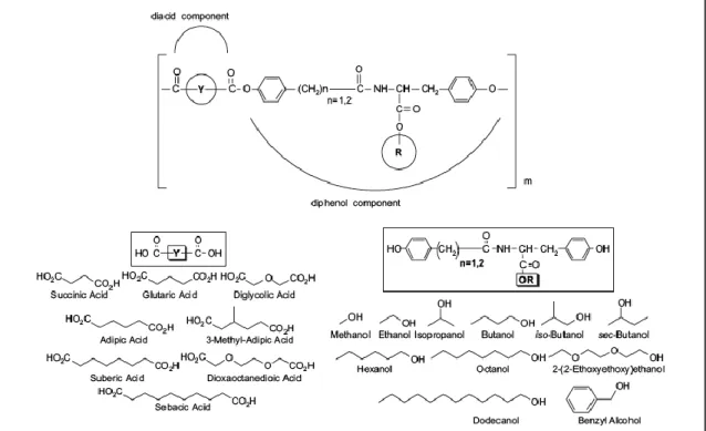
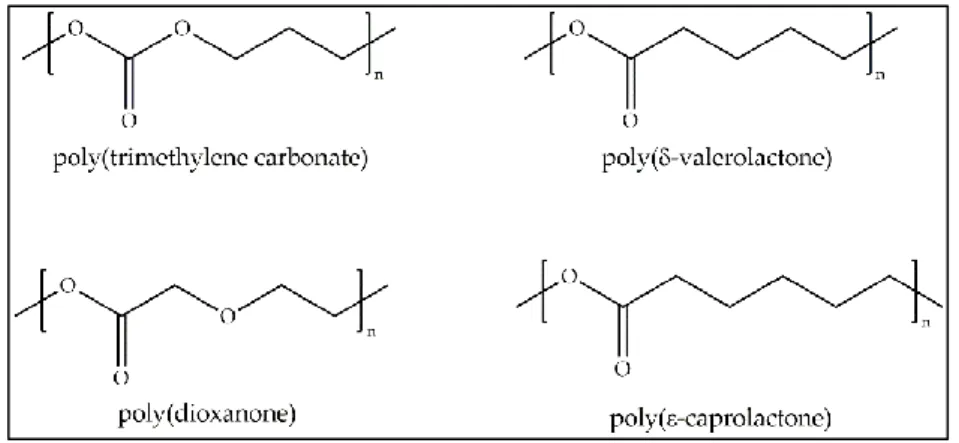
(9) Figure 2-5. Three-dimensional surface plot of water relative concentration with respect to time and relative distance. Note that the maximum value of relative concentration axis is 0.5. ................................................................................................................................ 29 Figure 3-1. Structure of L-tyrosine derived polyarylates. Symbol Y represents diacids (left) and symbol R represents tyrosine-derived diphenols (right). The number of methyl groups in the diphenol is variable (n = 1 for HTR, n = 2 for DTR) (L M Valenzuela, Michniak, & Kohn, 2011). ............................................................................................... 33 Figure 3-2. Example behavior of non-freezable water (𝑁𝑤𝑛𝑓, o), and freezable water (𝑁𝑤𝑓, •) in relation to 𝑊𝐶 of poly(DTH adipate). .......................................................... 34 Figure 3-3. Fg adsorption vs 𝑁𝑤 in polyarylates (a): non-freezable water. (b): freezable water. (•) high 𝑊𝐶, (o) low 𝑊𝐶. X-axes are not in same scale. ...................................... 36 Figure 3-4. Molecular structure of PEG. .......................................................................... 37 Figure 3-5. Water states distribution in PEG at different Mw. (•) Non-freezable water; (o) intermediate water. Modified from (Yamauchi & Tamai, 2003). .................................... 38 Figure 3-6. Proposed structure of water on hydrated PEG as shown in (H Kitano et al., 2001). Intermediate water showed in blue; non-freezable water showed in yellow. ....... 39 Figure 3-7. Proposed structure of water at the end of an hydrated PEG chain (peak X) as shown in (H Kitano et al., 2001). ..................................................................................... 40 Figure 3-8. Effect of PEG chain length, immobilized to PMMA, on platelet adhesion (•) and plasma protein adsorption (o). Modified from (Bergstrom et al., 1992). .................. 41 Figure 3-9. Molecular structure of aliphatic carbonyl polymers...................................... 42 Figure 3-10. Relation of intermediate water content and platelet adhesion in aliphatic carbonyl polymers. Data extracted from (Fukushima et al., 2015). ................................. 43 viii.

(10) Figure 3-11. Proposed structure of non-freezable (yellow) and intermediate (blue) water sorbed on PDO. Based on (Fukushima et al., 2015). ....................................................... 44 Figure 3-12. Molecular structure of PLGA and its monomers. ....................................... 45 Figure 3-13. Proposed structure of non-freezable water sorbed on PLGA. ..................... 46 Figure 3-14. Proposed structure of intermediate water sorbed on silk fibroin................. 47 Figure 3-15. Molecular structure of PVA. ....................................................................... 47 Figure 3-16. Water states distribution in PVA at different 𝑊𝐶. (•) Intermediate water; (o) non-freezable water; (▪) free water. Modified from (Hodge et al., 1996). ................. 48 Figure 3-17. Molecular structure of poly(meth)acrylates. ............................................... 50 Figure 3-18. Relation of intermediate water content and platelet adhesion in poly(meth)acrylates. Data extracted from (Tanaka, 2004). ............................................. 51 Figure 3-19. Molecular structure of PANcNVP and its monomers. ................................ 52 Figure 3-20. Relation of NVP content with platelet adhesion (•) and PRT time (o) on PANcNVP. Modified from (L. S. Wan et al., 2005). ....................................................... 54 Figure 3-21. Platelet adhesion on different polymers. ..................................................... 56. ix.

(11) NOMENCLATURE. ∆𝐻. Enthalpy change of melting of ice of bulk water. ∆𝐻𝑚. Enthalpy change of melting of ice. ∆𝐻𝑐𝑐. Enthalpy change of the cold-crystallization of ice. %Free. Weight percentage of free water. %Int. Weight percentage of intermediate water. %NF. Weight percentage of non-freezable water. Γ. Relation of permeability and diffusivity of water at interface. π. Non-dimensional permeability of the interface to water molecules. 𝐴. Amount of water that the interface is able to uptake at saturation. 𝐴𝑐. Calculated area of peak of NMR signal. 𝐴𝑚. Measured area of peak of NMR signal. 𝐴𝑤. Area of peak of NMR signal of pure water. ATR. Attenuated total reflection. 𝐶𝑒. Concentration of ester bonds. 𝐶𝑒0. Initial concentration of ester bonds. 𝐶𝑚. Concentration of monomers. 𝐶𝑤. Concentration of water. Cp. Specific heat capacity. 𝐷. Monomer diffusion coefficient. 𝐷𝑜. Monomer intrinsic diffusion coefficient. 𝐷𝑤. Water diffusion coefficient. DSC. Differential scanning calorimetry. 𝐸𝑊𝐶. Equilibrium water content. Fg. Fibrinogen. FT-IR. Fourier transform infrared. GA. Glycolic acid x.

(12) IR. Infrared. 𝑘1. Hydrolysis rate. 𝑘2. Acid-catalyzed hydrolysis rate. L. Thickness of the plate. LA. Lactic acid. 𝑀𝑝. Molecular weight per polymer repeating unit. MTDSC. Modulated differential scanning calorimetry. Mν. Viscosity-average molecular weight. 𝑀𝑤𝑎𝑡𝑒𝑟. Molecular weight of water. 𝑀𝑤. Molecular weight. 𝑀𝑤0. Initial molecular weight. 𝑛. Acid terminal group dissociation. NMR. Nuclear magnetic resonance. NVP. N-vinyl-2-pyrrolidone. 𝑁𝑤. Number of water molecules per polymer repeating unit. 𝑁𝑤𝑓. Number of free water molecules per polymer repeating unit. 𝑁𝑤𝑛𝑓. Number of non-freezable water molecules per polymer repeating unit. 𝑝. Intrinsic porosity. PAN. poly(acrylonitrile). PANcNVP. poly(acrylonitrile)-co-N-2-vinyl-pyrrolidone. PBA. poly(n-butyl acrylate). PCL. poly(ε-caprolactone). PDO. poly(dioxanone). PEA. poly(ethyl acrylate). 𝑃𝑒𝑎𝑘𝐻. Height of peak in NMR signal. 𝑃𝑒𝑎𝑘𝑊. Width of the peak in NMR signal. PEG. poly(ethylene glycol). PEHA. poly(2-ethylhexyl acrylate) xi.

(13) PGA. poly(glycolic acid). PHEMA. poly(2-hydroxyethyl methacrylate). PLA. poly(lactic acid). PLGA. poly(lactic-co-glycolic acid). PMEA. poly(2-methoxyethyl acrylate). PMMA. poly(methyl methacrylate). PPEA. poly(2-phenoxyethyl acrylate). PRT. Plasma recalcification time. PTMC. poly(trimethylene carbonate). PVA. poly(vinyl alcohol). PVL. poly(δ-valerolactone). 𝑄𝑐𝑐. Heat associated to cold-crystallization process. 𝑄𝑚. Heat associated to melting process. SEM. Scanning electron microscope. 𝑇𝑔. Glass transition temperature. TGA. Thermogravimetric analysis. 𝑊𝑈. Water content. 𝑤𝑑𝑟𝑦. Weight of dry sample. 𝑊𝑓. Mass of free water. 𝑤𝑓𝑟𝑒𝑒𝑧𝑎𝑏𝑙𝑒. Weight percentage of freezable water. 𝑊𝑖𝑛𝑡. Mass of intermediate water. 𝑊𝑛𝑓. Mass of non-freezable water. 𝑤𝑛𝑜𝑛𝑓𝑟𝑒𝑒𝑧𝑎𝑏𝑙𝑒 Weight percentage of non-freezable water 𝑤𝑝𝑜𝑙𝑦𝑚𝑒𝑟. Weight percentage of polymer. 𝑊𝑅𝑓𝑟𝑒𝑒𝑧𝑎𝑏𝑙𝑒. Weight ratio of freezable water:polymer. 𝑊𝑅𝑓𝑟𝑒𝑒𝑧𝑎𝑏𝑙𝑒. Weight ratio of non-freezable water:polymer. 𝑊𝑈. Water uptake. 𝑤𝑤𝑎𝑡𝑒𝑟. Weight of sorbed water xii.

(14) 𝑤𝑤𝑒𝑡. Weight of wet sample. XRD-DSC. X-ray diffraction with DSC. xiii.

(15) RESUMEN El agua cumple un rol fundamental en el funcionamiento de varias actividades biológicas en el cuerpo. En implantes poliméricos degradables, el agua forma parte del proceso de degradación a través de la hidrólisis. En superficies, el agua se comporta de manera distinta al analizarlo a niveles moleculares. Existen tres estados del agua en superficie: agua no-congelable, la cual no se congela incluso a -100°C; agua intermedia, la cual se congela a temperaturas bajo 0°C; y agua libre, la cual se congela a 0°C. Cuando un material es implantado en el cuerpo, lo primero que ocurre es la absorción de agua, seguido por el contacto con la sangre. La hemocompatibilidad corresponde al efecto de un material en la sangre o sus componentes, y se presume que el agua es capaz de influenciar la hemocompatibilidad de implantes poliméricos. Sin embargo, se sabe muy poco de esta relación. En este trabajo se estudiaron dos efectos del agua en polímeros: (i) el efecto en la cinética de degradación de polímeros, para lo cual se diseñó un modelo matemático de degradación de poliésteres; y (ii) el efecto en la hemocompatibilidad de polímeros, para lo cual se seleccionaron y analizaron distintos estudios de agua y hemocompatibilidad en polímeros. Se realizó una estimación de parámetros del modelo matemático de degradación a partir de datos experimentales de la literatura. Los valores obtenidos se encontraron dentro del rango esperado de valores según estudios anteriores, mientras que el modelo presentó un buen ajuste a los datos experimentales obtenidos de la literatura. Por otro lado, para estudiar el efecto del agua en la hemocompatibilidad se seleccionaron estudios de la literatura de cinco polímeros degradables y dos polímeros no-degradables. Se concluyó que contenidos de agua intermedia mayores a 3% peso están relacionados con mayor hemocompatibilidad en los casos de cinco de los siete polímeros analizados; en el caso de los otros dos, los datos disponibles no permitieron afirmar ni negar esta conclusión. Estos resultados muestran que: (i) el agua influencia la cinética de degradación y su comportamiento puede describirse mediante un modelo matemático; y (ii) que los estados del agua influencian la hemocompatibilidad de materiales poliméricos. Estos resultados otorgan información relevante para la selección, diseño y desarrollo de materiales poliméricos en la industria médica. xiv.

(16) ABSTRACT Water has a key role in the functioning of many biological activities in the body. In degradable polymeric implants, water takes part of the degradation process through hydrolysis. Water in surfaces presents different behavior at a molecular level and three states of water are recognized: non-freezable water, which does not freeze even at -100°C; intermediate water, which freezes below 0°C; and free water, which freezes at 0°C like bulk water. When a device is implanted in the body, water interacts first by adsorbing at the surface, followed by the contact with blood. Hemocompatibility is the effect of a material on blood or its components and it is presumed that water is capable to mediate hemocompatibility in polymeric devices. However, very little is known about this relation. This work focuses on two effects of water in polymers: (i) the effect on the polymer degradation kinetics, for which a mathematical model of polyester degradation was built; and (ii) the effect on polymer hemocompatibility, for which water and hemocompatibility studies in polymers available in literature were selected and analyzed. The parameters of the mathematical model were estimated from experimental data available in literature. The obtained values were in agreement to prior studies found in literature. On the other hand, to study the effect of water on hemocompatibility, studies available in literature of five degradable polymers and two non-degradable polymers were selected. It was concluded that intermediate water content higher than 3% wt is related to higher hemocompatibility for five of the seven polymer surfaces. For the remaining two polymers, no enough data was available to affirm or deny this conclusion. These results show that: (i) water influences the degradation kinetics and their behavior can be described through a mathematical model; and (ii) that the states of water influence the hemocompatibility of polymeric devices. These findings provide relevant information for polymer selection, design and development of polymeric materials in the medical field. Keywords: Intermediate water, non-freezable water, free water, water structure, platelet adhesion, fibrinogen adsorption.. xv.

(17) 1. 1.. INTRODUCTION. Water is considered the most important compound of life and it is the most abundant on earth. Over 70% of the surface of the planet is covered by water, in the form of solid, liquid and vapor (Robinson, 1996). It is also the main component of biological systems, being essential for many chemical reactions. Water is often regarded as the universal solvent because of its great versatility: it can dissolve proteins, ions, sugars, gases, organic liquids and lipids. What is fascinating about water is its uniqueness. Compared to other common liquids, water is characterized by having high boiling, melting and critical temperatures, large specific heat and high surface tension, among other properties (Ratner, 2012).. 1.1.. General aspects of water. Water is a small molecule composed by two hydrogen atoms covalently bonded to one oxygen atom. These bonds form a V-shaped structure with an angle of 104.6° (Figure 11) due to the two pairs of unused electrons of each oxygen atom, which tend to position as far from each other as they can to minimize the repulsion. The presence of these electrons causes a large dipole moment (i.e., uneven distribution of charges in the molecule), where the oxygen atom is slightly negatively charged, and the hydrogen atoms are slightly positively charged. This large dipole moment leads to a strong intermolecular interaction called hydrogen bonding, which is much weaker than the intramolecular covalent OH bond (23.3 kJ mol-1 vs. 492 kJ mol-1, respectively) (Chaplin, 2010). The most predominant form is the 4-coordinated water molecule which forms hydrogen bonds with four different water molecules, i.e., each hydrogen atom pairs up with an oxygen atom of different water molecules, while the oxygen atoms pairs up with two hydrogen atoms of different water molecules (Bagchi, 2013)..

(18) 2. Figure 1-1. Structure of a 4-coordinated water molecule. Hydrogen atoms are positively charged (δ+) and oxygen atoms are negatively charged (δ-), which also presents a lone pair of electrons. Solid lines indicate covalent bonds and dashed lines, hydrogen bonds. The behavior of pure water can be described by different models, which can be used to explain the peculiarities of water and its properties. In general, these models can be classified into two groups: (i) mixture or multicomponent models, where two or more water groups are present; and, (ii) continuum or uniformist models, in which each water molecule is influenced by the same intermolecular force (Jhon & Andrade, 1973). The flickering cluster model corresponds to a mixture model that suggests that clusters of hydrogen-bonded water are rapidly formed and swim in a medium of monomeric water molecules. However, this model fails to explain many of the water properties, as well as the nature of the clusters. On the other hand, the continuum model is a widely accepted model for water structure and explains water in terms of intact hydrogen bonds unlike the mixture model, where hydrogen bonds are broken between water molecules (Jhon & Andrade, 1973; Ratner, 2012)..

(19) 3. 1.2.. Water in biological systems. Water is very important in all biological systems. It is the major component of the body, with around 57% of the human weight. Without water, biochemical reactions would not be possible, as well as many other biological activities because these use water as their solvent. When medical devices are implanted in the body, the material is in contact with water before any other biological component, such as proteins or cells (Baier, 1978). Some of these devices are expected to degrade to allow cell regrowth in certain areas, such as bones or muscle. In many cases, they are made of polymers which degrade with the aid of water. Thus, it is reasonable to think that water plays a major role in material-body interactions in medical devices, specially mediating the biodegradation and biocompatibility of these materials (Ratner, 2012).. 1.2.1.. Biochemical reactions and body function. Water is fundamental in many biochemical reactions. For example, it is part of the enzymatic activity when a substrate binds to the active site displacing water molecules. The thermodynamics of this displacement contributes to the overall thermodynamics of protein-ligand binding (Nguyen, Cruz, Gilson, & Kurtzman, 2014). The same principle is observed in the association of antibodies with antigens, and hormones with biological receptors in cells (Lindstrom, 2008). Water also stabilizes the native state of protein and the double-helix form of DNA(Bagchi, 2013). At a larger scale, water helps in the mechanical function of the body. In articular cartilage, water helps in the lubrication and transportation of nutrients through the cartilage to chondrocytes, and the great load that the articular cartilage is able to support is due to the frictional resistance and the pressure gradient in the collagen-water matrix of the cartilage (Fox, Bedi, & Rodeo, 2009).. 1.2.2.. Swelling of Medical devices. Hydrophilic non-metallic medical devices implanted in the body swell by absorbing water onto their surface before any protein or cell approaches them. The amount of water.

(20) 4. uptaken by an implanted material is important for the material functioning as it impacts its degradation, interaction with blood and other biological components, its performance in tissue regeneration and the diffusion of molecules through the material. For example, the behavior of water affects the rate of dehydration of hydrogel based contact lenses and thus their performance (Ratner, 2012). In drug delivery systems, the slow release of drugs is due to the slow diffusion of water through the dry hydrogel matrix (J. Chen, Park, & Park, 1998). 1.2.3.. Polymer degradation. In some cases, polymeric medical devices and implants are expected to serve a supporting temporary purpose and then degrade and disappear. These devices are attractive because they are not required to be surgically removed after their objective is accomplished. Polymer degradation refers to the cleavage of covalent bonds which causes the scission in the polymer backbone and lateral chains forming oligomers and finally monomers. There are different degradation mechanisms, such as photo-, thermal-, mechanical and chemical degradation. Hydrolysis is the most common chemical process by which polymer degradation occurs and describes the reaction involving water and the functional group possessing the labile bond, then the rate of hydrolysis is influenced by the concentration of these two reactants (Göpferich, 1996).. The design of degradable devices requires long in vitro and in vivo experiments to ensure its safety until they get fully resorbed. Therefore, computer modelling offers a virtual and helpful alternative for testing, accelerating the design and development processes. Some models have been developed for polymer hydrolytic degradation. The most common are phenomenological models, which are based on diffusion-reaction equations, where the diffusion of the degradation products and the hydrolysis reaction are described. This type of mathematical models have been develop to predict the degradation kinetics of porous scaffolds (Y. Chen, Zhou, & Li, 2011; Heljak, Swieszkowski, & Kurzydlowski, 2014),.

(21) 5. fixation devices (Y. Wang, Pan, Han, Sinka, & Ding, 2008), and drug delivery devices (Y. Chen et al., 2011; Siepmann & Gopferich, 2001; Soares & Zunino, 2010).. 1.3.. Surface water. The water network can be disturbed by external elements such as ions, solutes and surfaces. When these elements get in contact with water, they reorganize its structure in order to minimize the energy of the system. In the case of surfaces, their interaction with water depends on properties such as structure, polarity, hydrophilicity or hydrophobicity, and composition of the surface. Water molecules reorder according to these factors, forming different conformations or layers on the vicinity of the surface. The influence of hydrophilic and hydrophobic surfaces on water structure has been widely studied as seen in the study by Li and collaborators, where the microscopic behavior of water on different surfaces of self-assembled monolayers was studied (Li, Du, & Yuan, 2013). They suggested that water molecules neighboring a hydrophilic surface are more rigid and have better ordering than pure water. In contrast, when faced with a hydrophobic surface, water molecules have almost the same mobility and distribution as of pure water.. The interaction of water molecules has an impact on different surfaces. Foods are often frozen to storage but their quality could be deteriorated after thawing because the change in texture due to the formation of ice. The higher the amount of tightly bound water, the less ice is formed in the food matrix, which contributes to better quality and stability of foods (Seetapan, Limparyoon, Fuongfuchat, Gamonpilas, & Methacanon, 2016). In metals, water is often believed to adsorb to the surface in a bilayer structure similar to ice structure (“ice-like water”). Noble metals, i.e. metals resistant to corrosion and oxidation, exhibit a weaker interaction with water molecules than less noble metals. This stable water bilayer can be regulated by changes in surface charge and influences the electrochemical performance of the metal (Schnur & Gross, 2009). For ceramics, those with higher surface energy interact with water molecules more tightly. The stabilization of this water.

(22) 6. molecules contributes to the overall stability of the hydrated ceramic-water system (Levchenko, Li, Boerio-Goates, Woodfield, & Navrotsky, 2006). In particular, on hydrated polymers, different water “types” or “states” have been observed. These can be classified depending on the mobility of water sorbed to the polymeric surface or its freezing temperature. Generally, there are three states of water, one with very low mobility and no freezing (even at -100°C); one with slightly higher mobility and freezing temperature below 0°C; and one with similar mobility and freezing temperature as bulk water.. 1.3.1.. States of water. The study of water in different surfaces has been driven by the interest in investigating the effects of water on the functionality of these surfaces. It includes hydrophobic/hydrophilic surfaces, metals, polymers, among others. Because of the large number of studies on this matter, a summary of the different denominations that water receives on surfaces is presented.. Generally, water is classified in three states according to mobility or freezing temperature criteria. Early studies using nuclear magnetic resonance (NMR) suggested the possibility of an ordered water structure in the vicinity of different surfaces, called bound or ice-like water due to its low molecular mobility. Later, other types of water were identified: one with higher mobility than the so-called bound water, and another that behaves similarly to bulk or pure water.. In most cases, the naming of the types of water has been based on its thermal behavior (i.e., crystallization), or on the mobility of their molecules (Table 1-1). Water can be classified according to low, intermediate and high mobility at atmospheric conditions, and based on this criterion Hechter and collaborators (Hechter, Wittstruck, McNiven, & Lester, 1960), Sterling and Masuzawa (Sterling & Masuzawa, 1968), and McBrierty and.

(23) 7. collaborators (McBrierty, Martin, & Karasz, 1999) got to the similar classification of the states of water with similar names. These three classifications were based on NMR spectra of water, which is described in the next section.. The other criterion used is the freezing temperature of water and the most common used denominations are the one presented by Higuchi and Iijima (Higuchi & Iijima, 1985), Hatakeyama and Hatakeyama (Hatakeyama & Hatakeyama, 1998), and Tanaka and collaborators (Tanaka et al., 2000). Non-freezing water does not freeze (even at -100°C); freezing bound water freezes at temperatures below 0°C; and free water freezes at 0°C. Hirata and collaborators (Hirata, Miura, & Nakagawa, 1999) described hydration water as the one that freezes below 0°C or does not freeze at all. Therefore, hydration water is equivalent to non-freezing and freezing bound water, while free water is the same in both cases. Additionally, the mobility and the freezing temperature criteria can be considered equivalent, because more thermal energy in molecules translates in faster movement of them and thus molecular mobility increases with temperature. A third criterion was proposed by Aizawa and collaborators (Aizawa & Suzuki, 1971), and Jhon and Andrade (Jhon & Andrade, 1973) that was based on the thermal expansion of water molecules and the transition temperature of this property, i.e., the temperature at which thermal expansion changes. Table 1-1. Denominations of the types of surface water based on different criteria.. Criteria. Rigidity and mobility. Types of water Name. Criteria. Ice-like watera. Very low mobility. Intermediate between icelike and free water b. Intermediate mobility. Free waterc. High mobility. Solid watera (glass-like or ice-like). Very low mobility. Reference. (Hechter et al., 1960). (Sterling & Masuzawa, 1968).

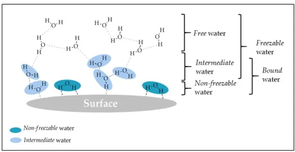
(24) 8. Freezing temperature. Thermal expansion. Bound waterb. Intermediate mobility. Free waterc (very loosely bound or liquid). High mobility. Tightly bound watera. Very low mobility at temperatures <230K. Loosely bound waterb. Low mobility in the range 230-260K. Free or bulk-like waterc. Mobility similar to bulk water at around 273K. Hydration waterd. Freezes sub-zero or does not freeze. Free watere. Freezes at 0°C. Bulk-like water. Normal mobility as normal melting point is approached. Non-freezing water or Nonfreezing bound waterf. No crystallization (no freezing). Freezing-bound water or Intermediate waterg. Crystallization under 0°C. Free watere. Normal crystallization of water. W3. Transition temperature: Non in -30 to 0°C. W2. Transition temperature: -20 to 0°C. W1. Transition temperature: 0°C. (McBrierty et al., 1999). (Hirata et al., 1999). (Hatakeyama & Hatakeyama, 1998; Higuchi & Iijima, 1985; Tanaka et al., 2000). (Aizawa & Suzuki, 1971; Jhon & Andrade, 1973). a. Ice-like water, solid water and tightly bound water are equivalent. Intermediate between ice-like and free water, bound water and loosely bound water are equivalent. c Free water in the three references are equivalent. d Corresponds to f+g. e Same free water by freezing temperature criterion. b. Here, the three types of water are referred as: non-freezable water, intermediate water and free water, according to the freezing temperature criterion. Non-freezable and intermediate water are bound water, while intermediate and free water are freezable water.

(25) 9. (Figure 1-2). In terms of structure and interaction with surfaces, the three water types are characterized by the following (Hatakeyama & Hatakeyama, 1998; Tsuruta, 2010): . Non-freezable water is tightly bound to the surface and the water-surface interactions are very strong, while water-water interactions are very weak.. . Intermediate water interacts moderately with the surface (stronger than free but weaker than non-freezable water), involving both water-surface and waterwater interaction.. . Free water hardly interacts with the surface and there is mainly water-water interaction.. Figure 1-2. Types of water on surfaces with the denominations, their structure and interactions on surfaces. 1.3.2.. Water measurement techniques. Water content and water uptake are two denominations for total water sorbed in a material. These can be can be measured by thermogravimetrical analysis (TGA), and their difference relies on whether they consider the dry or wet sample. Then, water uptake (𝑊𝑈) and water content (𝑊𝐶) can be calculated as follows:.

(26) 10. 𝑊𝑈 = 𝑊𝐶 =. 𝑤𝑤𝑎𝑡𝑒𝑟 𝑤𝑑𝑟𝑦 𝑤𝑤𝑎𝑡𝑒𝑟 𝑤𝑤𝑒𝑡. = =. 𝑤𝑤𝑒𝑡 −𝑤𝑑𝑟𝑦 𝑤𝑑𝑟𝑦 𝑤𝑤𝑒𝑡 −𝑤𝑑𝑟𝑦 𝑤𝑤𝑒𝑡. (1.1) (1.2). where 𝑤𝑤𝑎𝑡𝑒𝑟 , 𝑤𝑤𝑒𝑡 and 𝑤𝑑𝑟𝑦 , correspond to the weight of sorbed water, wet sample and dry sample, respectively.. There are several analytical methods to identify and/or quantify the different types of water on a surface. The three main techniques used are differential scanning calorimetry (DSC), NMR and infrared (IR) spectroscopy. These techniques are further described below.. 1.3.2.1.. Differential Scanning Calorimetry. The identification of the states of water on a surface and their quantities can be analyzed using DSC. It is widely used because the identification of intermediate water is easy due to the clear peaks associated with its phase transition. It has been used by Hatekayama and Hatekayama (Hatakeyama & Hatakeyama, 1998) to study the state of water in several insoluble and soluble polymers, such as cellulose, polyhydroxysterene, hyaluronic acid and poly(vinyl alcohol). Besides polymers, DSC can also be used to identify the states of water on metals (Johari, Hallbrucker, & Mayer, 1996), ceramics (Peng, Qisui, Xi, & Chaocan, 2009), and food (Tylewicz et al., 2016; Xu, Li, & Yu, 2014).. DSC allows the observation of the phase transitions in a thermogram from which various information can be extracted: (i) changes in heat capacity, (ii) magnitude of the heat (exothermic or endothermic), (iii) shape of the exotherms or endotherms, and (iv) the temperature at which these phenomena occur (McBrierty et al., 1999). Figure 1-3 shows a DSC thermogram of a hydrated surface containing the three types of water: nonfreezable, intermediate and free water. The exothermic peak below 0°C corresponds to cold-crystallization of water and indicates the presence of intermediate water. The.

(27) 11. endothermic peak at around 0°C corresponds to the melting of free water and intermediate water when it corresponds.. Figure 1-3. Scheme of a DSC thermogram of a hydrated surface with three states of water. Non-freezable water not visible in thermograms. Modified from (Tanaka, Hayashi, & Morita, 2013). The thermogram hands out useful information to calculate the amount of the types of water. The mass of intermediate (𝑊𝑖𝑛𝑡 ) and free water (𝑊𝑓 ) can be calculated according to the following equations: 𝑊𝑖𝑛𝑡 = 𝑊𝑓 =. 𝑄𝑐𝑐 ⁄∆𝐻 𝑐𝑐. 𝑄𝑚 ⁄∆𝐻 − 𝑊𝑖𝑛𝑡 𝑚. (1.3) (1.4). where ∆𝐻𝑐𝑐 and ∆𝐻𝑚 are enthalpy changes in the cold-crystallization and the melting of ice, respectively; and, 𝑄𝑐𝑐 and 𝑄𝑚 are the heat absorbed during the cold-crystallization process and the melting process, which are obtained from the area of the respective peaks in the thermogram. The enthalpy changes (∆𝐻𝑐𝑐 and ∆𝐻𝑚 ) are assumed to be the same as that of bulk water (334 J g-1) (Ping, Nguyen, Chen, Zhou, & Ding, 2001)..

(28) 12. The mass of non-freezable water (𝑊𝑛𝑓 ) is calculated as follows: 𝑊𝑛𝑓 = 𝐸𝑊𝐶(𝑤𝑡%) − 𝑊𝑖𝑛𝑡 − 𝑊𝑓. (1.5). where 𝐸𝑊𝐶 is the equilibrium water content of the sample.. The number of non-freezable (𝑁𝑤𝑛𝑓 ) and freezable (𝑁𝑤𝑓 ) water molecules per polymer repeating unit can be calculated using the DSC information, as previously described (Ping et al., 2001; Zhao et al., 2013). The weight ratio (𝑊𝑅𝑛𝑜𝑛𝑓𝑟𝑒𝑒𝑧𝑎𝑏𝑙𝑒 ) of non-freezable water/polymer, and the weight ratio (𝑊𝑅𝑓𝑟𝑒𝑒𝑧𝑎𝑏𝑙𝑒 ) of freezable water/polymer are to be calculated using the following equations: 𝑊𝑅𝑛𝑜𝑛𝑓𝑟𝑒𝑒𝑧𝑎𝑏𝑙𝑒 = 𝑊𝑅𝑓𝑟𝑒𝑒𝑧𝑎𝑏𝑙𝑒 =. 𝑤𝑛𝑜𝑛𝑓𝑟𝑒𝑒𝑧𝑎𝑏𝑙𝑒 𝑤𝑝𝑜𝑙𝑦𝑚𝑒𝑟. =. (𝐸𝑊𝐶−𝑤𝑓𝑟𝑒𝑒𝑧𝑎𝑏𝑙𝑒 ) 𝑤𝑝𝑜𝑙𝑦𝑚𝑒𝑟. 𝑤𝑓𝑟𝑒𝑒𝑧𝑎𝑏𝑙𝑒 𝑤𝑝𝑜𝑙𝑦𝑚𝑒𝑟. (1.6) (1.7). where 𝑤𝑛𝑜𝑛𝑓𝑟𝑒𝑒𝑧𝑎𝑏𝑙𝑒 , 𝑤𝑓𝑟𝑒𝑒𝑧𝑎𝑏𝑙𝑒 and 𝑤𝑝𝑜𝑙𝑦𝑚𝑒𝑟 , are the weight percentages of nonfreezable water, freezable water and polymer, respectively. 𝑤𝑓𝑟𝑒𝑒𝑧𝑎𝑏𝑙𝑒 is obtained from the DSC thermograms and calculated as follows: 𝑤𝑓𝑟𝑒𝑒𝑧𝑎𝑏𝑙𝑒 =. 𝑄𝑚 ∆𝐻𝑚. ∙ 100%. (1.8). Finally, 𝑁𝑤𝑛𝑓 and 𝑁𝑤𝑓 are obtained using the equations: 𝑁𝑤𝑛𝑓 = 𝑁𝑤𝑓 =. 𝑀𝑝 𝑀𝑤𝑎𝑡𝑒𝑟 𝑀𝑝 𝑀𝑤𝑎𝑡𝑒𝑟. ∙ 𝑊𝑅𝑛𝑜𝑛𝑓𝑟𝑒𝑒𝑧𝑎𝑏𝑙𝑒. ∙ 𝑊𝑅𝑓𝑟𝑒𝑒𝑧𝑎𝑏𝑙𝑒. (1.9) (1.10). where 𝑀𝑝 is the molecular weight per polymer repeating unit, and 𝑀𝑤𝑎𝑡𝑒𝑟 is the molecular weight of water..

(29) 13. 1.3.2.2.. Nuclear magnetic resonance. NMR is used to measure the dynamic behavior of water, in contrast to the static state of water that DSC measures. Most of the early investigations on water states used NMR for their identification, as in the case of Hechter and collaborators (Hechter et al., 1960) with agar gels. It can also be used for other materials such as muscle tissue (Fung & McGaughy, 1974) and food, including vegetables (Xu et al., 2014), fruits (Tylewicz et al., 2016), and dough (MacRitchie, 1976).. NMR is based on the line broadening observed when molecular mobility is interfered. For free water, the resonance lines result narrow, but when water molecules interact with a solid, the mobility of the molecules may be impeded or nonexistent on the NMR time scale, resulting in broad resonance lines (Schmitt, Flanagan, & Linhardt, 1994) (Figure 14). In general, a decrease in the signal intensity corresponds to an increased amount of bound water on the surface (Miwa, Ishida, Tanaka, & Mochizuki, 2010).. Figure 1-4. 2H-NMR spectra of water on a surface at different temperatures. The narrower peaks correspond to temperatures above 0°C, while broad lines correspond to temperatures below 0°C. Modified from (Miwa et al., 2010). The NMR spectra of the different water states are as follows (Miwa et al., 2010):.

(30) 14. . For non-freezable water the spectra is broad, showing low mobility due to strong interaction with the surface.. . For free water the spectra is narrow, very similar to bulk water, which means it has high mobility.. . For intermediate water the spectra is somewhere in between the spectra of the other two types of water, meaning that the mobility is intermediate.. The weight percentages of the different states of water can be calculated based on NMR data, though not many studies base their calculations on this technique. Sterling & Masuzawa (1968) presented the methodology to determine them. From the NMR signal, height (𝑃𝑒𝑎𝑘𝐻 ) of the peak and width (𝑃𝑒𝑎𝑘𝑊 ) at half the height of the peak are measured. Then, the area of the peak is measured: 𝐴𝑚 = 𝑃𝑒𝑎𝑘𝑊 ∙ 𝑃𝑒𝑎𝑘𝐻. (1.11). The width (𝑊𝑤 ) and the area (𝐴𝑤 ) of the peak of pure water are constant and considered 0.22 and 11.34, respectively. The calculated area (𝐴𝑐 ) of the peak of the sample is based on content of water in the sample: 𝐴𝑐 = 𝑊𝐶 ∙ 𝐴𝑤. (1.12). Then, the percentages of the water types can be calculated as follows: %𝑁𝐹 = 100 ∙ (1 −. 𝐴𝑚 𝐴𝑐. ). (1.13). %𝐼𝑛𝑡 = 100 − (%𝑁𝐹 + %𝐹𝑟𝑒𝑒) 𝑃𝑒𝑎𝑘𝐻 ∙𝑊𝑤. %𝐹𝑟𝑒𝑒 = 100 ∙ (. 𝐴𝑚. ). (1.14) (1.15). where %𝑁𝐹 , %𝐼𝑛𝑡 and %𝐹𝑟𝑒𝑒 correspond to the percentages of non-freezable, intermediate and free water, respectively..

(31) 15. 1.3.2.3.. Fourier transform infrared spectroscopy. Fourier transform infrared (FT-IR) spectroscopy is used to analyze the interaction of water molecules with functional groups of the surface. However, the information obtained cannot be used to calculate the amount of the different states of water. In general, IR analyzes the interaction of an infrared light with a molecule by detecting the energy absorbance or transmittance of the molecule due to its vibration. It is widely used to identify different molecules or molecular structure because functional groups vibrate at different energy levels (Stuart, 2004). The O-H stretching band region at around 38003000 cm-1 is of much interest because the interaction with water occurs through hydrogen bonding. Shifts of the wavenumber are associated to a change of the hydrogen bonding strength: the stronger the hydrogen bond, the lower the wavenumber shift (Morita, Tanaka, & Ozaki, 2007). FT-IR can be used in conjunction to attenuated total reflection (ATR) to analyze thin samples (Tanaka et al., 2013). With ATR-IR the infrared beam passes through a crystal, reflecting with the surface in contact with the sample positioned on top of it. The reflection produces an evanescent wave that goes through the sample. When the sample absorbs energy from the evanescent wave, this is attenuated, and the attenuated beam is analyzed to obtain the IR spectra.. 1.3.2.4.. Other techniques. Other techniques have been used to study the types of water on surfaces. Raman spectroscopy can be used to analyze the structure and hydrogen bonding of sorbed water and it is similar to IR. Raman spectroscopy detects changes in the polarizability of the molecular bonds, whereas IR detects changes in the dipole moment. The analysis extracted from these two are complementary and therefore provide a better insight of the water structure (Hiromi Kitano et al., 2005). Recent research has been developed to clarify the origin of cold-crystallization of water combining wide-angle X-ray diffraction with DSC (XRD-DSC) (Kishi, Tanaka, & Mochizuki, 2009). The XRD determines the atomic and.

(32) 16. molecular structure of a crystal by the diffraction of incident X-rays, which with the combination of DSC allows identification of the origin of phase transition.. 1.4.. Biocompatibility. Biocompatibility is defined as “the ability of a material to perform with an appropriate host response in a specific application” (Williams, 1987). This definition includes the characteristics that is expected for a material to have: (i) the material in the body must have a specified function and therefore it has to perform it; (ii) the host response that the material provokes has to be acceptable; and (iii) the response to a specific material will vary in different situations because the performance of the material depends on a specific application, in a specific tissue (Williams, 1999, 2012). Given that biocompatibility changes according to the situation, it should not be considered as a property of a biomaterial, but a characteristic of a material-tissue interaction (Williams, 2012).. There are several factors that affect biocompatibility. Some of them are composition of the material, production processes, structure (e.g., woven, knitted, polished, film, tube, sponge, sphere), surface characteristics (e.g., smoothness, porosity, rheology), surface treatments/coatings, location of the device, and expected host response on the interface (e.g., macrophage activation, biofilm formation, encapsulation, platelet adhesion) (Williams, 2012). Considering these factors a more detailed definition of biocompatibility was proposed by Williams (Williams, 2012): “Biocompatibility refers to the ability of a biomaterial to perform its desired function with respect to a medical therapy, without eliciting any undesirable local or systemic effects in the recipient or beneficiary of that therapy, but generating the most beneficial cellular or tissue response in that specific situation, and optimizing the clinically relevant performance of that therapy.”. Biocompatibility evaluation can be performed analyzing different biological effects that the material has in the body. The assessment of biocompatibility according to the ISO.

(33) 17. 10993 (U.S. Department of Health and Human Services, Food and Drug Administration, 2016) is based on the material characteristics and its potential risk in the body under the conditions it is used. The biocompatibility test categories presented by the ISO 10993 are: hemocompatibility, cytotoxicity, degradation, implantation, sensitization, irritation or intracutaneous reactivity, acute system toxicity, material-mediated pyrogenicity, subacute or subchronic toxicity, genotoxicity, chronic toxicity, carcinogenicity, and reproductive or developmental toxicity.. Hemocompatibility is the effect of a material on blood or blood components such as breakdown of blood cells, immunologic response and thrombus formation. In this work, hemocompatibility is evaluated by the adsorption of plasma proteins and platelet adhesion. It is known that when an implant takes contact with blood, plasma proteins adsorb to the surface. Fibrinogen (Fg), albumin and immunoglobulins are the most abundant, and along with fibronectin, vitronectin and the von Willebrand factor, these proteins are mediators of the platelet adhesion and thrombosis around the biomaterial (Badugu, Lakowicz, & Geddes, 2004). In particular, fibrinogen, the main protein in blood plasma, is fundamental in blood coagulation and thrombosis induced by biomaterials. Activation of fibrinogen leads to platelet immobilization, activation and aggregation, although the availability of platelet-binding sites is more important than the total amount of adsorbed fibrinogen in mediating platelet adhesion (Badugu et al., 2004). Either way, high fibrinogen adsorption and high platelet adhesion imply that the biomaterial is not inert in blood, hence it has low hemocompatibility.. Before an implant takes contact with blood, water is firstly sorbed onto the surface, thus it is presumed that water plays a fundamental role in material-body interactions. However, only few studies consider water on the surface as a relevant factor on biocompatibility, and even fewer relate its states on the surface with its hemocompatibility. Studying the relation between water states and hemocompatibility of materials will allow to predict the body response against the implanted material..

(34) 18. 1.5.. Hypothesis and Objectives. Water on hydrated polymers influences polymer degradation and hemocompatibility, and the presence of the states of water (i.e. non-freezable, intermediate and free water) plays a key role in blood-material interactions. The two general objectives of this study and their specific aims are: 1. To design a mathematical model that describes polymer degradation including the effect of water that can relate to biological response. 1.1. To construct a mathematical model that includes the effect of water on polymer degradation. 1.2. To estimate the parameters of the models and verify the model with experimental data available in literature. 2. To study the relation between water and its states on polymer surfaces with their hemocompatibility, specifically fibrinogen adsorption and platelet adhesion. 2.1. To select relevant studies of the states of water and hemocompatibility on polymers from literature. 2.2. To assess the cause of the formation of water states on polymers. 2.3. To evaluate the relation between water states and hemocompatibility on selected polymers. This study is expected to describe the effect of water on polymer degradation through mathematical modelling. On the other hand, it is expected to provide a deeper insight on the hydration states of water and their relation with the biocompatibility of polymeric devices by analyzing the effects of the presence or absence of the states of water on fibrinogen adsorption or platelet adhesion in different polymers. These findings will present relevant information that will aid in the process of polymer selection for medical devices and polymeric materials design..

(35) 19. 1.6.. Organization of the Document. The present document is organized as follows. Section 2 describes the construction of the degradation model, its results and discussion. Section 3 presents the effect of water on hemocompatibility found in each polymer which are divided in two groups: degradable and non-degradable polymers. Then, the obtained results are discussed in three separated topics: (i) states of water in polymers, (ii) platelet adhesion on polymers, and (iii) effect of water states in polymers on biological response. Finally, Section 4 highlights the main conclusions of this study and the future challenges on this field. The annex includes the article submitted to the International Journal of Molecular Sciences. It is important to clarify that all experimental data presented in this document was extracted from literature and not obtained directly by the author..

(36) 20. 2.. MATHEMATICAL MODEL OF POLYMER DEGRADATION AND WATER UPTAKE. The degradation of polymeric devices is of special interest in tissue regeneration and drug delivery applications. As the polymer degrades, biological components take over the device and allows regeneration. Once polymeric devices are implanted in the body, their degradation rate are influenced by water uptake, protein adsorption and cellular adhesion (Woo, Chen, & Ma, 2003). Among the most commonly degradable polymers in industry are polyesters, which correspond to a group of polymer containing ester groups in their main chains. Current research applications of synthetic degradable polyesters comprise drug delivery, sutures, orthopedic and dental implants and fixation devices (Ratner, 2012). Poly(glycolic acid) (PGA), poly(lactic acid) (PLA) and their copolymers correspond to the most investigated and used aliphatic polyesters in the biomaterial field. The hydrophobicity of lactic acid reduces the water uptake decreasing the degradation rate as compared to PGA. These polymers degrade by hydrolysis of the ester bond, which can also be catalyzed by acidic or basic groups or enzymes (Dunne, Corrigan, & Ramtoola, 2000). The hydrolysis of PGA, PLA and their copolymers can be catalyzed by their own degradation products or monomers (autocatalysis) because these correspond to acidic groups. In the bulk of the polymeric matrix, the reduction of pH accelerates the degradation process by accumulation of acidic degradation products. Computer modelling of polymer degradation helps the design process of degradable materials and shortens the times of device development. Phenomenological models based on reaction-diffusion equations are the most common among mathematical models. They describe the hydrolysis reaction and the diffusion of degradation products through the polymer matrix. For a drug delivery application, Soares & Zunino (2010) presented a mixture model that describes water-dependent degradation and erosion of polymers, as well as drug release from the polymer. They analyzed the polymer as a polydisperse system, i.e., a system constituted by a collection of molecules of different sizes instead of solely by molecules of a single chain size. By making this consideration they were able to account for different diffusion rates of chains with different sizes through the polymer.

(37) 21. matrix. Y. Wang et al. (2008) presented a phenomenological model for the degradation of PGA, PLA and their copolymers, used in orthopedic fixation with various geometries. They based their model on the existing understanding of biodegradation mechanisms: hydrolysis, autocatalysis and diffusion. In other studies, they included the interaction between crystallization and degradation and the analysis of the mechanical properties of the polymers (Pan, 2014). In this work, a mathematical model based on the two models mentioned (Soares & Zunino, 2010; Y. Wang et al., 2008) was developed, which describes the effect of water content on the degradation mechanisms of aliphatic polyesters, specifically PGA, PLA and their copolymers used for tissue regeneration. The aim of adding water to this model was to mathematically relate polymer degradation to biological response because, as mentioned above, the degradation rate is influenced by protein adsorption and cellular adhesion, where water acts as a mediator of this interaction.. 2.3.. Model Formulation. The mathematical model developed is based on the one proposed by Y. Wang et al. (2008), which involves the reaction and diffusion phenomena of the species in the polymer degradation process. In their study, the species considered were monomers, as product of the degradation, and ester bonds. In this work, water was also considered as it is relevant for hydrolysis and can also be related to biological response. Two main assumptions were made: (i) size distribution of polymer chains and hydrolysis products are ignored, i.e. monomers, and (ii) the degree of crystallinity of the polymers is assumed to be constant.. The model is formed by a system of partial differential equations describing the concentration of monomers, ester bonds and water in time. The governing equation for monomer concentration is as follows: 𝑑𝐶𝑚 𝑑𝑡. 𝑛 = 𝑘1 𝐶𝑒 𝐶𝑤 + 𝑘2 𝐶𝑒 𝐶𝑚 + 𝛻(𝐷𝛻𝐶𝑚 ). (2.1).

(38) 22. where 𝐶𝑚 is the monomer concentration, 𝑡 is time, 𝑘1 is the hydrolysis rate, 𝐶𝑒 is the ester bond concentration, 𝐶𝑤 is the water concentration, 𝑘2 is the acid-catalyzed hydrolysis rate, 𝑛 is the acid terminal group dissociation (equal to 0.5) and 𝐷 is the monomer diffusion. Monomer concentration depends on the production of monomers by uncatalyzed hydrolysis (first term) and by autocatalyzed hydrolysis (second term). The term in the right corresponds the diffusion of monomers through the polymer matrix, assuming Fick’s laws for diffusion. The diffusion coefficient D can be related to the porosity of the matrix by the following equation: 𝐷 = 𝐷𝑜 (1 + 𝛼𝑝). (2.2). where 𝐷𝑜 is the intrinsic diffusion coefficient and 𝑝 is the intrinsic porosity. Here, 𝛼 is an empirical parameter and its value is fixed at 4.5 by Y. Wang et al. (2008). The porosity is generated by the loss of short chains (Pan, 2014) and can be estimated as: 𝑝 = 1−. 𝐶𝑚 +𝐶𝑒. (2.3). 𝐶𝑒0. where 𝐶𝑒0 corresponds to the initial concentration of ester bonds. Then, equation 2.1 can be rewritten as: 𝑑𝐶𝑚 𝑑𝑡. 𝑛 = 𝑘1 𝐶𝑒 𝐶𝑤 + 𝑘2 𝐶𝑒 𝐶𝑚 + 𝛻 {𝐷𝑜 [1 + 𝛼 ( 1 −. 𝐶𝑚 +𝐶𝑒 𝐶𝑒0. )] 𝛻𝐶𝑚 }. (2.4). The reduction of ester bond concentration is given by the un-catalyzed hydrolysis and the acid-catalyzed hydrolysis of polymer chains. Then the governing equation for ester bond concentration is as follows: 𝑑𝐶𝑒 𝑑𝑡. 𝑛 = −(𝑘1 𝐶𝑒 𝐶𝑤 + 𝑘2 𝐶𝑒 𝐶𝑚 ). (2.5). The ester bond concentration relates to the molecular weight of the polymer matrix in the following manner: 𝐶𝑒 𝐶𝑒0. 𝑀. = 𝑀𝑤. 𝑤0. (2.6).

(39) 23. Water concentration depends on the un-catalyzed hydrolysis and the diffusion of water through the polymer matrix, as shown in the next equation: 𝑑𝐶𝑤 𝑑𝑡. = −𝑘1 𝐶𝑒 𝐶𝑤 + 𝛻(𝐷𝑤 𝛻𝐶𝑤 ). (2.7). where 𝐷𝑤 corresponds to water diffusion.. 2.3.1.. Initial conditions. Before any degradation has taken place in the polymeric matrix, no monomer has been produced and its concentration is zero, i.e. 𝐶𝑚 (𝑥, 𝑡)|𝑡=0 = 0 , while ester bond concentration was considered as the initial molecular weight of the polymer matrix, i.e. 𝐶𝑒 (𝑥, 𝑡)|𝑡=0 = 𝑀𝑤0 . As the matrix starts out dry, 𝐶𝑤 (𝑥, 𝑡)|𝑡=0 = 0.. 2.3.2.. Boundary conditions. At the center of the plate (x = 0) no diffusion of any specie (monomers, ester bonds and water) occurs through this boundary. Then: 𝜕𝐶𝑚. |. 𝜕𝑥 𝑥=0. = 0,. 𝜕𝐶𝑒. |. 𝜕𝑥 𝑥=0. = 0,. 𝜕𝐶𝑤. |. 𝜕𝑥 𝑥=0. =0. for t > 0.. (2.8). At the border of the plate (x = L), where L corresponds to the thickness of the plate, monomers diffuse from the center of the matrix to the border due to concentration gradient, and their concentration is close to zero 𝐶𝑚 (𝑥, 𝑡)|𝑥=𝐿 = 0. For ester bonds, i.e. oligomers, the border of the plate is impermeable, then. 𝜕𝐶𝑒. |. 𝜕𝑥 𝑥=𝐿. = 0.. In the case of water, it permeates through the interface according to the following boundary condition (Soares & Zunino, 2010): [𝐷𝑤. 𝜕𝐶𝑒 𝜕𝑥. + Γ π (𝐶𝑤 (𝑥, 𝑡)|𝑥=𝐿 − 𝐴)] = 0. (2.9).

(40) 24. where π corresponds to the non-dimensional permeability of the interface to water molecules and 𝐴 to the amount of water that the interface is able to uptake at saturation, i.e. the equilibrium WC (EWC). Γ corresponds to a non-dimensional number that relates the permeability and diffusivity of water at the boundary: 𝐿π. Γ=𝐷. (2.10). 𝑤. 2.4.. Simulation. The simulation of the model was performed using the software Matlab® and the pdepe function, which solves parabolic-elliptic partial differential equations. A one-dimensional case was considered utilizing experimental data presented by (Grizzi, Garreau, Li, & Vert, 1995) of a 2 mm thick PLA plate.. 2.4.2.. Parameter estimation. From the experimental data obtained from (Grizzi et al., 1995), five parameters of the model (Water model) and the three parameters of the original model (Wang’s model) were estimated (Table 2-1). The input data corresponded to the initial molecular weight, the EWC of the polymer and the thickness of the sample, extracted from the experimental data.. Table 2-1. Estimated parameters and R2 of degradation and water uptake data of the Water model and Wang’s model.. Parameter 𝐷0 𝑘1. Unit 𝑚2 𝑤𝑒𝑒𝑘 3 𝑚 ( ⁄𝑚𝑜𝑙 ) 𝑤𝑒𝑒𝑘. Water Model. Wang’s model. 8.70 x 10-7. 3.90 x 10-8. 1.30 x 10-3. 2.53 x 10-5.

(41) 25. 3 √𝑚 ⁄𝑚𝑜𝑙. 2.50 x 10-3. 2.43 x 10-3. 4.83 x 10-11. --. 2.38 x 10-5. --. R2 degradation. 0.98. 0.99. R2 water. 0.81. --. 𝑘2 𝐷𝑤 π. 𝑤𝑒𝑒𝑘 𝑚2 𝑤𝑒𝑒𝑘 𝑚2 𝑤𝑒𝑒𝑘. Comparing the estimated parameters for both models, shown in Table 2.1., the diffusion rate of monomers (𝐷0 ) of the Water model is one order of magnitude greater than Wang’s model, which means that monomers exit the polymer matrix faster probably because the water in the polymer accelerates diffusion. The auto-catalyzed hydrolysis rate (𝑘2 ) in both cases are similar, while the non-catalyzed hydrolysis rate (𝑘1 ) of the Water model is two orders of magnitude greater than the other. This could be due to the more relevant role that was given to water in the first model causing a greater contribution to the degradation rate than in the second one. Also, as monomer diffuse at slower rate in Wang’s model this could result in a higher concentration of monomers in the polymer matrix causing more auto-catalyzed hydrolysis than non-catalyzed, as opposed in the Water model, where monomers diffuse faster to the outside of the matrix..

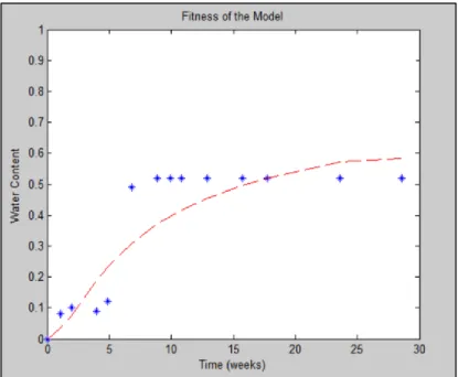
(42) 26. Figure 2-1. Comparison between the experimental (blue asterisks) and predicted (dashed lines) degradation as functions of time. Red lines: Water model, R2 = 0.98; blue lines: Wang’s model, R2=0.99. Experimental data obtained from (Grizzi et al., 1995).. Figure 2-1. shows the fitness of both models according to the estimated parameters. Both models have a good fit with the experimental data (the value of R2 of the Water model and Wang’s model are 0.98 and 0.99, respectively). In figure 2-2. the fitting of the Water model with water concentration data is shown. Here, the value of R2 is 0.81, the fitting accuracy is lower than degradation prediction. Other border conditions describing water behavior at the interface are to be tested to obtain a better fitting of the model..

(43) 27. Figure 2-2. Comparison between the experimental (blue asterisks) and predicted by the Water Model (red dashed lines) water content as functions of time. R2=0.81. Experimental data obtained from (Grizzi et al., 1995). 2.4.3. Species distribution evolution in polymer matrix A three-dimensional surface plot for each three variables (𝐶𝑚 , 𝐶𝑒 and 𝐶𝑤 ) was obtained (Figures 2-3 to 2-5) using the Water Model. In these figures the behavior of monomers, ester bonds and water concentration with respect to time and relative distance from the center of the plate are observed. Analyzing the surface plots, one can observe that the three species behave according to what is expected to physically occur within the polymer matrix. Monomer concentration (Figure 2-3) is zero at the beginning of the degradation and increase until a maximum value coinciding with the depletion of ester bonds. Then, the concentration starts to decrease in time and within the matrix as monomers diffuse to the outside of it. Ester bond concentration (Figure 2-4) decreases rapidly throughout the matrix because the EWC is reached in a short period of time. At the border, ester bonds accumulate because of the impermeable border condition but the plot also shows that ester bonds concentration is undefined, thus the mathematical problem, i.e. border condition, related should be fixed..

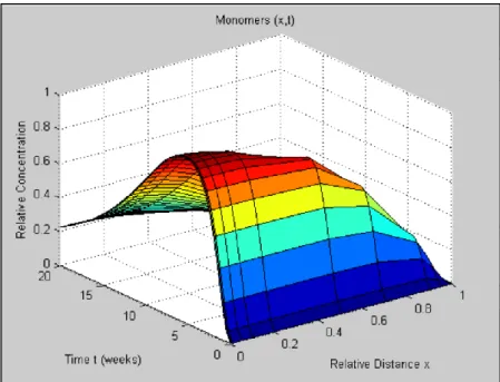
(44) 28. Figure 2-3. Three-dimensional surface plot of monomer relative concentration with respect to time and relative distance.. Figure 2-4. Three-dimensional surface plot of ester bond relative concentration with respect to time and relative distance..

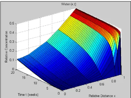
(45) 29. Water (Figure 2-5) reaches its maximum concentration very fast at the border according to the experimental data and then, it slowly diffuses through the matrix to the center. According to the estimated parameters, the permeability rate (π) is higher than the water diffusion rate (Dw ) (2.48 x 10-5 and 4.83 x 10-11, respectively), therefore the rapid water uptake and slow water diffusion to the center are expected. However, because water concentration is low at x = 0 and t = 0, the degradation should be slower than at the outer sections of the matrix, as oppose what is shown in Figure 2-4. There are two possible causes for this misbehavior: (i) water actually diffuses faster through the polymeric matrix being available for hydrolytic degradation in the entire matrix, or (ii) degradation, i.e., ester bond concentration decrease, is not considering local concentration of water but total amount of water in the matrix.. Figure 2-5. Three-dimensional surface plot of water relative concentration with respect to time and relative distance. Note that the maximum value of relative concentration axis is 0.5..

(46) 30. 2.5.. Conclusions. In this section, a mathematical model for polymer degradation was presented. This model included the contribution of water in the degradation process in order to relate it to the biological response. The design of this model was based on a previous degradation model, which was modified adding water in the degradation process. After the construction of the model, experimental data of PLA degradation previously reported was used for parameter estimation of the two models. Both models fit well to the experimental data and the parameter values agreed with the degradation and diffusion kinetics of the polymer matrix. Three-dimensional surface plots of the Water model were analyzed and, in general, monomers, ester bonds and water concentration behaved according to what is expected.. This model was able to describe PLA degradation, however further simulation is needed to verify its accuracy in other polyesters such as PGA and copolymers, which present different degradation and water uptake kinetics. Also, degradation experiments can be carried out to obtain empirical values of the parameters and validate the model.. Polymer degradation is also influenced by biological response, such as protein adsorption and cell adhesion. Since water is the responsible for the interaction of polymeric devices and biological components, the mathematical model presented here can be further modified and improved to describe the effect that these components have on the degradation. From current available data, it is not possible to obtain a mathematical relation between these. In the next section, a thorough analysis of the effect of water on the hemocompatibility of polymers is presented, which will shed the first light on the relation between degradation, water and biological response, for future development of this model..

(47) 31. 3. 3.1.. EFFECT OF WATER ON HEMOCOMPATIBILITY OF POLYMERS Study Selection and Data Analysis. Different water and hemocompatibility studies on polymers were selected from the literature. In the case of water, the selection was restricted to studies with available data on the content of water states or DSC thermograms within a temperature range from about -100°C to above 0°C. For hemocompatibility studies, the selection was based on the polymers which water studies were selected before. The type of sample structure of the polymer (film or hydrogel) was also considered in the selection.. The contents of non-freezable, intermediate and free water were directly extracted from the selected studies, as well as hemocompatibility data. Other relevant information on the sample characteristics, such as molecular weight, sample weight, sample fabrication, were recorded. When water states data was not available, it was obtained by the analysis of DSC curves of the polymer. The content of freezable (intermediate and free) and nonfreezable water were calculated with equations 1.1, 1.2 and 1.6 to 1.10 as described by Ping et al. (2001) and Zhao et al. (2013).. 3.2.. Results on the effect of the states of water on hemocompatibility. From the selected studies, data of water states and hemocompatibility of five degradable polymers (L-tyrosine derived polyarylates, poly(ethylene glycol) (PEG), a group of aliphatic carbonyls, and poly(lactic-co-glycolic acid) (PLGA)) and two non-degradable polymers (poly(meth)acrylates and poly(vinyl alcohol)s (PVAs)) were extracted and calculated. In this section, the analysis and discussion of the impact of water states on the hemocompatibility (i.e. protein adsorption or platelet adhesion) of each polymer is presented. Also, a brief description of the characteristics and current applications of each polymer is included..

(48) 32. 3.2.1. 3.2.1.1.. Degradable polymers L-tyrosine derived polyarylates. L-tyrosine-derived polyarylates are a family of 112 A-B-type copolymers with an alternating sequence of tyrosine-derived diphenol and an aliphatic diacid. These were firstly synthesized by Kohn and collaborators (Brocchini, James, Tangpasuthadol, & Kohn, 1997; Fiordeliso, Bron, & Kohn, 1994) (Figure 3-1). For this library, the number of oxygen or carbon atoms in the polymer backbone and pendent chain affects properties such as the glass transition temperature (Tg) and the water contact angle. These polymers have been used to fabricate bone pins showing no significant inflammatory response in in vivo resorption studies (Hooper, Macon, & Kohn, 1998). Also, drug eluting implants near the eye area have been fabricated (“Lux Biosciences Gains Exclusive Worldwide License for Polyarylate Patent Estate From Rutgers University for Ophthalmic Use,” 2006), as well as FDA approved devices for hernia repair and infection control in 2006 (“FDA approves first medical device using Rutgers biomaterial,” 2006). Recently, potential topical psoriasis therapy using drug loaded nanospheres have been developed which are based on amphiphilic block copolymers of PEG and L-tyrosine-derived polyarylate oligomers (Kilfoyle et al., 2012)..

(49) 33. Figure 3-1. Structure of L-tyrosine derived polyarylates. Symbol Y represents diacids (left) and symbol R represents tyrosine-derived diphenols (right). The number of methyl groups in the diphenol is variable (n = 1 for HTR, n = 2 for DTR) (L M Valenzuela, Michniak, & Kohn, 2011). Previously, the influence of different properties of polymeric films on their 𝑊𝑈 behavior was investigated, due to the high variability of the latter reported in various studies (L M Valenzuela et al., 2011). From this study, the DSC curves for 21 of the used polymers were obtained, along with the 𝑊𝑈 data. From the former, the sample weight and the enthalpy change of the melting process of freezable water (𝑄𝑚 ) were extracted. Then, the 𝑊𝐶 and the number of freezable (𝑁𝑤𝑓 ) and non-freezable (𝑁𝑤𝑛𝑓 ) water molecules per polymer repeating unit were calculated, as described in section 2.2.1. Depending on the 𝑁𝑤𝑓 , polymers were classified into two groups: (i) low 𝑊𝐶, from 0 to 0.31 and 𝑁𝑤𝑓 less than 10, and (ii) high 𝑊𝐶, from 0.45 to 0.6 and 𝑁𝑤𝑓 more than 10..

(50) 34. The analysis of the behavior of 𝑁𝑤𝑛𝑓 and 𝑁𝑤𝑓 related to the 𝑊𝐶 of the polymer shows that the majority of them have similar behavior (Figure 3-2), where 𝑁𝑤𝑛𝑓 rises until a threshold from which it tends to remain constant, while 𝑁𝑤𝑓 keeps rising as the polymer absorbs more water. However, when 𝑊𝐶 is very low (around 0.05) 𝑁𝑤𝑛𝑓 is higher than 𝑁𝑤𝑓 . This probably occurs because at lower 𝑊𝐶 the total amount of water is close to the amount of non-freezable water allowed in the polymer, and freezable water is in smaller or similar amounts. Also, in Figure 3-2, 𝑁𝑤𝑓 does not reach any saturation point like 𝑁𝑤𝑛𝑓 because the calculation were performed considering data until reaching the maximum 𝑊𝐶 of the polymer.. Figure 3-2. Example behavior of non-freezable water (𝑁𝑤𝑛𝑓 , o), and freezable water (𝑁𝑤𝑓 , •) in relation to 𝑊𝐶 of poly(DTH adipate). Fibrinogen adsorption data was obtained from Weber and collaborators (Weber, Bolikal, Bourke, & Kohn, 2004) (Table 3-1). Figure 3-3 shows the relation between 𝑁𝑤 and fibrinogen adsorption of non-freezable and freezable water. In the case of non-freezable water, there is no apparent relationship between the fibrinogen adsorbed to the surface, but for the low 𝑊𝐶 group there is a tendency to increase as the amount of water is increased. On the other hand, when only freezable water is analyzed, the low 𝑊𝐶 group has the same tendency as the previous case, although the correlation is lower in the latter..