Macroecological factors explain large scale spatial population patterns of ancient agriculturalists
10
0
0
Texto completo
(2) Macroecological patterns of ancient agriculturalists INTRODUCTION Understanding the spatial patterns of distribution and abundance of species at regional, continental and global scales is a central goal in biogeography and macroecology. To date, such macroscale patterns have been explained by a variety of mechanisms, ranging from environmental constraints to biotic interactions (Brown et al., 1996; Araújo & Luoto, 2007; Elith & Leathwick, 2009; Reino et al., 2013). Humans also play an important role in shaping the distribution of a wide range of taxa. In contrast to the extensive research efforts that have been devoted to the impacts of humans on other organisms, human beings per se as a unique species (Homo sapiens) are far less understood in terms of macroscale patterns and their driving factors. Indeed, this issue is rarely the focus of ecologists, because the study of humans has long been the preserve of the humanities and social sciences. However, H. sapiens is, in principle, governed by the same physical, chemical and biological laws as any other species. The idea that human–environment relationships at macroscales can be explained by ecological principles gives rise to the emerging field of ‘human macroecology’, which employs large datasets and statistical tools to address issues related to human ecology at large spatial and temporal scales (Burnside et al., 2012). Although still new, this paradigm has already contributed valuable insights into various important aspects of human societies, such as demographic growth, public health, cultural diversity and sustainability (Burger et al., 2012; Burnside et al., 2012; Amano et al., 2014; Brown et al., 2014). One essential question in human macroecology would be how to understand the patterns of distribution and abundance of human populations and their driving mechanisms at macroscales. Previous studies have demonstrated the potential value of using ecological theories and approaches to unravel these patterns at particular social stages. In hunter-gatherer societies, for example, population structure can be explained through the use of well-established ecological principles involving environmental capacity, resource use and intraspecific interactions (Hamilton et al., 2007). Actually, the idea that human populations and sociocultural patterns are constrained by ecological factors is not new in the field of palaeoanthropology. Recent applications of ecological niche modelling have provided useful insights into such important palaeoanthropological topics as the extinction of the Neanderthals (Homo neanderthalensis), the dispersal of prehistoric human populations and the development of cultures (Banks et al., 2008, 2013; Varela et al., 2011). In comparison, for present-day humans one might intuitively think that the role of ecological factors is rather minor, because highly organized social structures and developed technologies can buffer the constraints of the physical environment in particular regions or societies. However, this is not necessarily true if we look at larger scales. For example, in the modern era, the global abundance of the human population and global distribution of human land use are found to be strongly correlated with climate, topography and other environmental factors (Small, 2004; Beck & Sieber, 2010; Samson et al., 2011). This implies the possibility that, at macroscales, the spatial pat-. terns of humans are substantially driven by similar ecological mechanisms to the spatial patterns of other species. Despite probable exceptions in specific situations, this possibility deserves further investigation. It would be particularly interesting to ask whether, and determine the extent to which, ecological mechanisms can act as ‘universal’ explanations for macroscale patterns of distribution and abundance of human as well as those of other species. During the past two millennia, most humans have lived in agrarian societies. Agriculturalists feed primarily on crop foods, and crop yield has always been dependent on environmental conditions such as climate, topography, soil type and the availability of water resources (Lobell & Field, 2007; Licker et al., 2010; Van Wart et al., 2013). Restrictions of these environmental conditions can be mitigated by technological solutions that enhance the efficiency of resource use and resolve problems related to the scarcity of local resources. However, in premodern agrarian societies, with a relatively low level of technology, crop yield would depend strongly on environmental conditions. In this sense, the environmental factors that influence the availability of food resources are, in turn, likely to determine population size at large spatial scales. For example, previous time-series analyses have shown that agrarian societies in China, as well as the whole Northern Hemisphere, primarily experienced a collapse of their populations when the climate in a given region became more unfavourable for agriculture. Therefore, one plausible explanation suggests that population collapse is essentially caused by climatic changes that reduce the carrying capacity of agrarian lands (Lee et al., 2009; Lee & Zhang, 2010; Zhang et al., 2011). Another striking example of such an ‘environment–resource–population’ relationship is illustrated by the collapse of the Mayan civilization in Mesoamerica; an appealing explanation of this collapse is that the feedback between demographic growth and resource depletion eventually led the system to a tipping point triggered by drought (Tainter, 1988; Hodell et al., 1995; Janssen & Scheffer, 2004). Here, we propose the following hypotheses to explain macroscale patterns of agriculturalist population density in relation to climate, topography and resource availability. These three factors have been repeatedly identified as the primary determinants of species distribution and abundance at macroecological scales. 1. Population density typically has a hump-shaped relationship with climate, showing an optimum at ‘moderate’ climatic conditions. This corresponds to the existing abundant-centre hypothesis in ecology (Hengeveld & Haeck, 1982; Brown, 1984), which postulates that the highest species abundance occurs at intermediate niche space positions. This hypothesis also makes intuitive sense, as extremely hot/wet or cold/dry environments are not suitable for crop cultivation, and thus not suitable for denser human settlements. 2. Lowland areas can support higher population densities than mountainous areas, because complex topographic relief increases the cost of agricultural land use, resulting in a lower per unit area yield of crop. In general, such a negative. Global Ecology and Biogeography, 24, 1030–1039, © 2015 John Wiley & Sons Ltd. 1031.
(3) C. Xu et al. topographic effect may also hold for other human activities (e.g. transportation), leading to lower population densities. 3. Population density is positively correlated with local resource availability for food production, particularly in terms of soil and surface water resources. Areas with better soil conditions, which can facilitate crop growth, and surface water resources, which can facilitate agricultural irrigation and the production of foods from aquatic sources, have higher population densities. In addition, the formation of a population centre and the resulting trend of a large-scale concentration of population towards such a centre is a common phenomenon in many societies. This type of population centre is often located at an administrative or economic centre, but not necessarily at the geographic centre, of a population. This spatial structure of population concentration could be driven purely by socioeconomic processes. For instance, it could originate from a central-place foraging mode among sedentary human populations, and could be reinforced by the positive feedbacks of socioeconomic processes such as the production of scale economies. Meanwhile, this population-concentration structure could be a result of environmental effects if the environment also presents such a spatial structure. At a minimum, we aim to test for the spatial trends of population concentration toward a primary monocentre of population at a national level. This trend serves merely as a null model demonstrating the extent to which this simplistic structure can capture the actual patterns of population distribution. Multiple population centres or clusters may be observed in many cases; however, they are not considered in our study in order to avoid extra assumptions related to socioeconomic processes that are required for the identification and explanation of such multiple centres. China fostered one of the oldest civilizations in the world. Situated in the mid-latitudes of East Asia, it spans broad environmental gradients. The earliest agricultural activities in China may date as far back as 8000 to 10,000 bce, and agrarian societies were dominant before China entered the periods of the imperial dynasties, starting in 221 bce. Many of China’s dynasties preserved detailed records, including demographic census data. Such historical data provide us with an opportunity to look at human population patterns at large spatial scales over nearly 2000 years. Here, we test the three above-mentioned hypotheses, together with an analysis of the spatial structure of large-scale concentrations of population, by statistically modelling population density in ancient China in relation to a relevant set of environmental variables. METHODS Ancient population data China became unified as a nation for the first time in 221 bce and was subsequently ruled by multiple imperial dynasties. Agrarian societies dominated the majority of China and no systematic large-scale emigration overseas occurred before the 1840s (Lee et al., 2009), which makes the ancient Chinese population a suitable focus for our study. For the purpose of main1032. taining governance, systematic demographic censuses were conducted during most dynasties, although data are lacking for some short-lived dynasties. The economic historian Fangzhong Liang made an exhaustive compilation of census data by administrative unit (Liang, 1980), which was used as the main data source for reconstructing population patterns in the present study. We restricted our study area to between 20 and 40° N and 96 and 122° E, which roughly separates Chinese agricultural civilization from that of the nomadic tribes/nations. Also, we excluded time periods when the study area (representing the majority of China) was not unified or was ruled by short-lived dynasties (see Appendix S1 in Supporting Information). Finally, we retained the 13 periods when stable agrarian societies were present (i.e. agriculturalists dominated Chinese society, and no large-scale social conflicts occurred either during or shortly before these periods). In this way, we were able to focus on agriculturalists living in relatively stable social settings. By digitizing and georeferencing (using an equal area Lambert projection) the Historical Atlas of China (Tan, 1982), we derived the geographic boundaries of the administrative units and matched them with the census data to map population density between 2 and 1820 ce. The resulting population density maps were then converted to 100 km × 100 km grid cells (Fig. 1). Environmental variables Nine candidate explanatory variables were chosen and quantified for each grid cell (Table 1). Specifically, mean annual temperature and precipitation (Hijmans et al., 2005) were used to represent climatic conditions. Mean topographic slope and standard deviation of elevation were used to quantify topographic relief. Sand fraction, available water storage capacity and the total organic matter content of topsoil (0–30 cm) were selected as easily interpretable indicators of soil properties (FAO/IIASA/ISRIC/ISSCAS/JRC, 2012). The density of hydrological systems, defined as the total shore length of lakes and rivers within a given grid cell, was used to quantify the availability of surface water resources, because the exploitation of surface water for agricultural purposes is largely restricted to the accessible riparian areas. In addition, we used ‘cost distance’ to the administrative centre (i.e. the national capital) to characterize the population-concentration structure at a national scale in each period studied. Cost distance is a measure of the difficulty of moving between two locations: each grid cell is assigned an impedance value and the easiest transportation path from a source site to the destination is represented by the path with the least accumulated impedance, the value of which is defined as cost distance (Adriaensen et al., 2003). Elevation has been frequently used to measure the landscape impedance of animal movement (Zeller et al., 2012). Cost distance is thus a simple proxy of the impedance of human migration, based on the assumption that the difficulty of migration through a given grid cell is positively correlated with its elevation. Because spatial data of the past environments are not available for the historical periods that correspond to our population dataset, we used modern environmental data as surrogates in the. Global Ecology and Biogeography, 24, 1030–1039, © 2015 John Wiley & Sons Ltd.
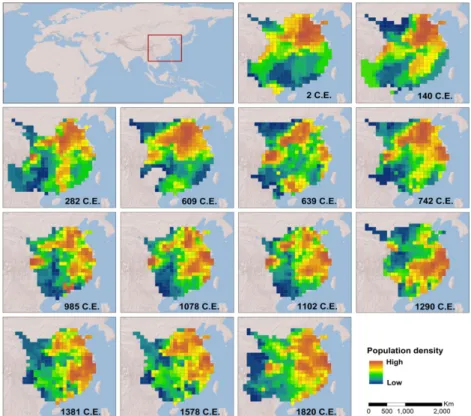
(4) Macroecological patterns of ancient agriculturalists. Figure 1 Location of study area and human population density per 100 km × 100 km grid cell in the 13 studied periods from 2 to 1820 ce. Population densities are derived from historical census data (Liang, 1980) and the Historical Atlas of China (Tan, 1982).. Table 1 Candidate explanatory variables and data sources. Model. Variable. Unit. Data source. Scale/resolution. Climate. Mean annual temperature Mean annual precipitation Mean slope Standard deviation of elevation Sand fraction Available soil water storage capacity Soil organic matter content Density of hydrological systems. °C mm degree – % mm m−1 % km km−2. 1 km × 1 km 1 km × 1 km 1 km × 1 km 1 km × 1 km 30 arcsec 30 arcsec 30 arcsec 1:1,000,000. Cost distance to administrative centre. –. WorldClim WorldClim SRTM elevation data SRTM elevation data Harmonized world soil database v.1.2 Harmonized world soil database v.1.2 Harmonized world soil database v.1.2 China hydrological map from National Geomatics Center of China SRTM elevation data. Topography Resource quality. Concentration. 1 km × 1 km. SRTM, Shuttle Radar Topography Mission.. quantification of explanatory variables. This was based on the consideration that large-scale (at 100 km × 100 km) geographic patterns of these variables should remain relatively stable over the periods studied, despite the possibility of substantial temporal variations in their absolute values. For each studied period we reconstructed the spatial distribution of temperature (Appendix S2), which is probably one of the most sensitive candidate variables. Very similar results were obtained from the reconstructed and modern temperature data (Table S2), which can (partly) justify the use of such a surrogate for the past environment. Statistical analyses We used simultaneous autoregressive (SAR) models to account for the spatial autocorrelation (SAC) that generally occurs in. grid cell-based macroecological datasets. Among the various statistical techniques used to deal with SAC, the simultaneous autoregressive (SAR) model has been shown to generally perform well (Dormann et al., 2007). Of the three types of SAR model (i.e. spatial error model, lagged model and mixed model), the lagged model (SARlag, assuming that the autoregressive process only occurs in the response variable) was selected for our study based on the assumption that the SAC structure is generated, apart from the explanatory variables, by endogenous processes (i.e. domestic population migration). This is the case for similar distance-related biotic processes, such as reproduction, dispersal or geographic range extension (Legendre, 1993; Diniz-Filho et al., 2003). The SAR error model has been suggested to perform better on the basis of tests using an artificial dataset (Kissling & Carl, 2008);. Global Ecology and Biogeography, 24, 1030–1039, © 2015 John Wiley & Sons Ltd. 1033.
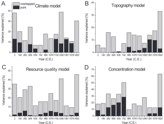
(5) C. Xu et al. however, our case is robust to the selection of SAR models, since very similar results (not shown) can be obtained from different model types. Before the analyses, population density as a response variable was log-transformed to avoid highly skewed distributions. We first examined pairwise relationships between population density and each explanatory variable using a SAR-based univariate regression (Appendix S3). We then constructed SAR models to separately test for the effects of climate, topography, land resource quality and population concentration (namely the climate, topography, resource quality and concentration models, respectively). Quadratic terms of both temperature and precipitation were included in the climate model to test for hump-shaped effects. Temperature and precipitation were also separately modelled to compare their effects. Our hypotheses are complementary to each other, allowing us to combine the climate, topography, resource quality and concentration models into a full model to quantify the total variation explained by all these effects at one time. Overall, we fitted seven classes of SAR models, including the four aforementioned models plus two submodels of climate (i.e. the temperature and precipitation models) and a full model. The model selection procedure was performed based on the Akaike information criterion (AIC) and coefficient of determination (R2). We calculated the variance inflation factors (VIF) of the explanatory variables. All VIFs for the variables in each model had a value of less than five, indicating very weak multicollinearity. With regard to the existing debate on spatial regression (Hawkins, 2012), we also fitted an ordinary least squares (OLS) model to allow for a comparison between spatial and nonspatial models (Appendix S4). We evaluated the model fit by comparing both R2 and the Akaike weight (ωi), considering that the information-theoretic approach can be complemented with conventional statistical testing. To assess the relative importance of the studied effects, variation partitioning was used to quantify the variation that can be purely explained by an individual class of explanatory variables (i.e. the ‘pure’ effect) and also the joint effects between different sets of variables (i.e. the ‘overlapped’ or ‘shared’ effects) (Legendre & Legendre, 2012). To do this we decomposed the SAR models into a spatial signal and a non-spatial trend, and only the nonspatial components were used in variation partitioning because we focused on the effects of the explanatory variables rather than on their effects mixed with space. We quantified the total variation explained by all examined effects using a full model that combined the retained variables of all individual SAR models. In this case, the increasing multicollinearity of variables will not be a problem because we only focused on the explanatory power. The pure and overlapped explanatory power of each individual effect was quantified using the pseudo R2 of non-spatial components of the SAR models, defined as the squared Pearson correlation coefficient between the nonspatial component of the SAR prediction and observed values. The statistical analyses were implemented in R 3.1.1 with the spdep package (Bivand et al., 2014). 1034. R E S U LT S Spatial patterns of ancient Chinese populations manifest clear temporal variations over the studied periods (Fig. 1). In the relatively early periods, the population was primarily aggregated in the North China Plain where Chinese civilization originated. During the following two millennia, several spatial shifts of high-density population clusters occurred that can be visually identified from the population density maps, such as the southward and northward shifts into the Yangtze and North China plains, respectively. All hypothesized human–environment relationships can be well fitted using SAR models, as shown by the high coefficient of determination R2 of 70–90% (Table 2). Such a high explanatory power is largely attributed to the internal SAC of population density. The pseudo-R2 of the non-spatial components of the SAR models reflects the variation captured by individual classes of explanatory variables. In general, climate (temperature + precipitation, R2 c. 5–40%), topography (R2 c. 1–35%), land resource quality (R2 c. 10–45%) and population-concentration structure (R2 c. 10–65%) can all explain a substantial proportion of the variation in population patterns, and together (i.e. the full models) they capture c. 25–65% of the total variation. However, variation partitioning shows that their explanatory powers largely overlap with each other (Fig. 2), indicating that the hypothesized mechanisms can jointly explain the observed patterns in most cases. Closely scrutinizing the pairwise relationships separately reveals the effects of each explanatory variable (Appendix S3). In line with our first hypothesis, population density shows a hump-shaped relationship (indicated by the negative quadratic terms) with both temperature and precipitation. These two climatic variables jointly influence population density, but temperature generally outweighs precipitation in terms of R2 and Akaike weights (ωi) (Table 2). In most studied periods, negative effects are found from the topographic variables, suggesting that increasing topographic relief can restrict population density, which agrees with our second hypothesis. Despite the generally weak explanatory power of topography, occasional exceptions exist in which the topographic model has a fairly high likelihood of being the best model (i.e. 1381 ce and 1578 ce). We also found positive relationships between population density and soil water storage capacity, sand fraction, as well as density of hydrological systems, suggesting that a persistent role exists for soil and surface water in supporting agriculturalist populations. Apart from those environmental effects, the simple spatial structure of the concentration of population also shows a highly consistent effect across time, which can explain considerable variations in population density, presenting the best model with the largest ωi value in five out of the 13 studied periods (Table 2). DISCUSSION Although the idea that biogeographic determinants may underlie human civilizations has been around for decades (Lamb,. Global Ecology and Biogeography, 24, 1030–1039, © 2015 John Wiley & Sons Ltd.
(6) 0.15 0.13 0.01 0.11 0.10 0.06 0.80 0.89 0.01 0.01 0.02 0.04 0.48 0.49 0.29 0.38 0.52 0.33 0.46 0.28 0.30 0.33 0.49 0.38 0.36 0.64 0.89 0.91 0.83 0.88 0.80 0.88 0.81 0.91 0.88 0.87 0.80 0.74 0.90 0.39 0.01 0.41 0.14 0.60 0.91 0.00 0.00 0.00 0.01 0.42 0.33 0.02 0.18 0.19 0.34 0.26 0.33 0.51 0.10 0.18 0.16 0.28 0.13 0.13 0.64 0.89 0.81 0.83 0.88 0.80 0.87 0.81 0.91 0.87 0.87 0.81 0.75 0.90 0.13 0.55 0.18 0.68 0.26 0.00 0.00 0.00 0.00 0.98 0.06 0.18 0.49 0.36 0.21 0.29 0.33 0.12 0.16 0.16 0.25 0.17 0.41 0.11 0.10 0.46 0.89 0.91 0.83 0.88 0.81 0.88 0.80 0.91 0.87 0.87 0.81 0.75 0.90 0.08 0.01 0.21 0.02 0.02 0.01 0.19 0.11 0.99 0.00 0.37 0.40 0.00 0.06 0.04 0.16 0.13 0.01 0.07 0.16 0.14 0.13 0.08 0.14 0.18 0.33 0.89 0.91 0.83 0.88 0.81 0.88 0.81 0.91 0.88 0.87 0.81 0.75 0.90 0.04 0.06 0.07 0.04 0.01 0.01 0.00 0.00 0.00 0.00 0.01 0.01 0.00 0.38 0.20 0.12 0.25 0.07 0.07 0.18 0.14 0.18 0.39 0.14 0.11 0.31 0.89 0.91 0.83 0.88 0.81 0.88 0.80 0.91 0.87 0.87 0.81 0.75 0.90 0.09 0.22 0.02 0.00 0.00 0.00 0.00 0.00 0.00 0.00 0.06 0.02 0.00 0.28 0.14 0.01 0.17 0.07 0.01 0.02 0.02 0.01 0.29 0.07 0.00 0.01 0.89 0.91 0.84 0.88 0.81 0.88 0.81 0.91 0.88 0.87 0.81 0.75 0.91 0.13 0.03 0.10 0.01 0.01 0.01 0.00 0.00 0.00 0.01 0.06 0.04 0.00 0.89 0.91 0.84 0.89 0.81 0.88 0.81 0.91 0.87 0.87 0.81 0.75 0.90 2 140 282 609 639 742 985 1078 1102 1290 1381 1578 1820. 0.31 0.18 0.05 0.13 0.06 0.08 0.07 0.10 0.16 0.28 0.07 0.09 0.32. NS R2 R2 ωi NS R2 R2 ωi NS R2 NS R2. ωi. R2. Concentration model Resource quality model Topography model. R2 ωi NS R2 R2 ωi NS R2 R2 ωi NS R2 R2 Year (ce). Climate model (temperature plus precipitation) Precipitation model Temperature model. Table 2 Model performance shown by the pseudo-R2 of the simultaneous autoregressive models (total R2 and the non-spatial components NS R2) and Akaike weights (ωi).. Full model. ωi. Macroecological patterns of ancient agriculturalists 1982; Diamond, 1997), evidence supporting this concept based on quantitative analysis remains largely insufficient. A major part of the world’s population over the past millennia has consisted of agriculturalists. This is still the case in many regions to the present day. Our understanding of the history and future development of human societies can increase based on the quantification of large-scale patterns and potential determinants of socio-economic traits of agrarian societies (Turchin & Nefedov, 2009; Beck & Sieber, 2010). By using high-quality, recently developed data sources and spatial modelling techniques, our study provides useful insight into this issue from a macroecological perspective. Our results support the formulated hypotheses on the relationships between agriculturalists and the environment, and help to unravel the mechanisms shaping agriculturalist patterns. The foremost finding of our study is that populations of ancient agriculturalists have had conspicuous correlations with environmental factors over the last 2000 years, suggesting that physical environments have, to a considerable extent, determined the population patterns of agriculturalists. This finding clearly demonstrates that our own species is constrained by several macroecological factors, and that even our substantially developing capability for ecological engineering cannot exempt us from these constraints over an extended period of time and history. Our results suggest the possibility that there are certain similar ecological mechanisms underlying the formation of macroscale patterns for both H. sapiens and other species. One plausible mechanism rests on the extended ‘abundant-centre’ hypothesis. In line with the theoretical prediction that the highest abundance of species occurs at optimal conditions in the ecological niche space, we found that agriculturalists consistently had their largest densities at intermediate levels of temperature and precipitation in all studied periods. The growth of the main crops in China, including rice and wheat, can be stressed by either insufficient or excessive heat and/or water. Earlier studies modelling the climatic niches of these crops indeed show hump-shaped suitability along these climatic gradients (Appendix S5). In this sense, the climatic constraints that control crop production are also effectively the macroscale constraints of agriculturalist populations even though this effect may be tempered by storage and transport capacities at relatively small scales. This climate–agriculturalist relationship is roughly confirmed by the substantially overlapping spatial ranges of clusters of high population and areas presenting high climatic suitability of the main crops (Appendix S5). Also, approximate congruence can be observed between the reconstructed past cropland patterns (Kaplan et al., 2010; Klein Goldewijk et al., 2011) and our reconstructed population patterns. This congruence can further support our hypothesis, although it cannot serve as a robust confirmation because of the inherent feedback between agriculturalists and croplands. Among the three classes of environmental factors tested in our study, climate had the largest pure effect (Fig. 2) in determining the macroscale patterns of agriculturalist populations. The dominant role of climate has been perceived in general as a control on species distributions at large spatial scales (Pearson &. Global Ecology and Biogeography, 24, 1030–1039, © 2015 John Wiley & Sons Ltd. 1035.
(7) A. overlapped Climate model pure. B. 40. Variance explained (%). C. Xu et al.. 30. Topography model. Variance explained (%). 40. 30. 20. 10. 0. 20. 10. 0 2. 140 282 609 639 742 985 107811021290138115781820. 2. Year (C.E.). Year (C.E.). Resource quality model. 50. D Variance explained (%). Variance explained (%). C. 140 282 609 639 742 985 107811021290138115781820. 40. 30. 20. 10. Concentration model. 70 60 50 40 30 20 10. 0. 0 2. 140 282 609 639 742 985 107811021290138115781820. 2. 140 282 609 639 742 985 107811021290138115781820. Year (C.E.). Year (C.E.). Figure 2 Result from variation partitioning among the climate, topography, resource quality and concentration models. Variations that can be solely explained by a focal individual model (pure, black bars) and that can be jointly explained by all four models (overlapped, grey bars) were quantified based on the non-spatial components of the simultaneous autoregressive models.. Dawson, 2003). Moreover, our results indicating the relative importance of energy and water agree with previous work based on a time-series analysis showing that in ancient Chinese societies population size was primarily determined by temperature (Lee et al., 2009); however, our study also reveals an interesting similarity between H. sapiens as an agriculturalist species and other species in the sense that energy generally acts as the principal determinant at macroscales (Hawkins et al., 2003). Our topographic hypothesis is mainly based on the fact that wheat and rice have been the primary food resources of Chinese populations over a long history. The production of these crops that support human populations strongly depends on cultivation practices, which were largely constrained by topographic conditions in the pre-industrial era. Our hypothesized negative topographic effect is supported by our results. However, such an effect may not be observed in other regions of the world. For example, some important crops such as potatoes and corn originated in mountainous areas, and their production is much less constrained by topographic conditions. In this sense, topographic constraints may not operate through limiting crop production in areas where these crops are the major food resources. Our three hypotheses reflect the environmental effects on food availability for agriculturalists. By supporting these hypotheses, our results suggest that food resources are likely to be a direct factor shaping species abundance patterns, and this is common to H. sapiens and other species. Recent studies have increasingly acknowledged the significance of biotic interactions 1036. in driving macroecological patterns (Araújo & Luoto, 2007). In particular, as an important type of biotic interaction across trophic levels, dietary resources are found to play a substantial role in this context (Kissling et al., 2007). In an ecological sense, feeding on other species creates a fundamental interaction between H. sapiens and food species, and this type of interaction is probably more important for agriculturalists than any other type of biotic interaction. Therefore, one would expect to find evidence of the dependence of agriculturalist patterns on the environmental conditions that determine the abundance of food resources. Albeit not very surprising, this result has an important implication that similar ecological relationships plausibly occurs between human beings and other (consumer) species. Apart from these observed environmental correlations, a simple spatial population structure that shows a concentration of humans toward national capitals can also capture a portion of the patterns of agriculturalist populations. Note that the variations explained by the concentration model substantially overlap with other models that characterize environmental effects, suggesting that the concentration structure could be partly attributed to environmental gradients. Accurately disentangling the relative strengths of environmental versus socioeconomic effects would prove difficult without more detailed data. Nonetheless, our analyses indicate that equal attention should be paid to both types of effect in future research efforts to acknowledge the dual nature of human beings.. Global Ecology and Biogeography, 24, 1030–1039, © 2015 John Wiley & Sons Ltd.
(8) Macroecological patterns of ancient agriculturalists Multiple lines of evidence discovered from numerous sites of both ancient and current civilizations world-wide suggest that environmental factors often play a fundamental role in human occupation and the development and collapse of human societies (Diamond, 2005; Butzer, 2012). Meanwhile, much debate exists on this issue, since markedly diverse environmental effects emerge when evidence is gathered at a small scale (e.g. site-level evidence) from different geographic locations and cultures. For instance, humans generally select regions with a mild climate and plain lowlands to establish settlements, but dense occupation can also be found in rather ‘harsh’ environments such as mountainous Mexico (Caballero et al., 2002) and the high Andes (Núñez et al., 2002). Note that these exceptions are not contradictory to our findings, because of the large difference in observation scale. It has been well recognized that determinants of species distribution/abundance can substantially shift with scale (Elith & Leathwick, 2009). Our study can provide a large-scale view on our own species, which is necessary to complete our current understandings of human– environment relationships that are mostly based on small-scale observations. Supported by our results, we speculate that macroecological constraints (e.g. climate and topography) will definitely have a substantial influence on human populations in a similar way to their affect on other species, if observations are taken at adequately large scales (e.g. a continental or global scale). Some caveats need to be acknowledged in our study. Although our assumption that the large-scale patterns of environmental variables remained stable over the two millennia may be sound, it is very difficult to validate because spatial information on historical environments is not available at the scale of our study. The explanatory power of the models has apparent temporal variations (Fig. 2); however, we neither recognize any clear trend nor have any definite explanations for this from the present study. Some specific social events may have driven the agriculturalist patterns and diluted the environmental effects during particular periods, and these were not considered in this study as it was beyond our scope. Interestingly, spatio-temporal dynamic features of agriculturalist densities should be noted. For example, a clear southward shift of high-density population clusters took place from 1102 to 1290 ce (Fig. 1). The explanation from a historical view would be that the frequent, intense wars during a dynastic change (in this case from the Song to Yuan dynasties) caused the reduction and southward migration of populations in northern China. However, a simple logistic model taking into account environmental effects can offer an ecological explanation for dramatic population changes (Lima, 2014). Intuitively, the shift in population patterns could be induced by climatic cooling during that time period that caused agricultural conditions to deteriorate in northern wheat production and pastoral regions; this made it impossible for the landscape to support dense human populations (Lee et al., 2008). Our study serves as a starting point in the analysis of macroecological patterns of humans; a detailed investigation into the spatio-temporal dynamics in this context is an area for further research.. We may gain important insight into present and future of human societies by learning from history. Climate change has been demonstrated to be associated with a series of general crises in human history (Hodell et al., 1995; Lee & Zhang, 2010; Zhang et al., 2011); such change has also been suggested to be part of the reason for some social conflicts in recent decades (Burke et al., 2009; Hsiang et al., 2011). Our results showing the agriculturalist–environment relationships have useful implications that will allow a better understanding of the consequences of global environmental change for human well-being in the future (Dearing et al., 2010), since currently about half of the world’s people still live in agricultural populations. This is still the case in many regions where people are strongly dependent on local to regional food production regardless of whether they themselves are involved in agriculture or are living in an agrarian society. Follow-up studies that address macroscale spatial patterns of humans and their associated driving mechanisms are encouraged because they will support policy-making decisions related to adaptation to profound environmental changes.. ACKNOWLEDGEMENTS We thank Sheng Sheng and Ting Chi for assistance in preparing the dataset on the ancient Chinese population. We also appreciate two anonymous referees for their valuable comments on an earlier version of the manuscript. C.X. is supported by Natural Science Foundation of China (41271197) and China Scholarship Council. B.J.W.C. is supported by China Scholarship Council (2010619022). S.A. is supported by ICM-MINECOM, P05-002 IEB. L.R. received support from the Portuguese Ministry of Education and Science and the European Social Fund, through the Portuguese Foundation of Science and Technology (FCT), under POPH – QREN – Tipology 4.1 (post-doc grants SFRH/BPD/62865/2009 and SFRH/BPD/93079/2013). L.R. was also supported by the project “Biodiversity, Ecology and Global Change” co-financed by North Portugal Regional Operational Programme 2007/2013 (ON.2 – O Novo Norte), under the National Strategic Reference Framework (NSRF), through the European Regional Development Fund (ERDF) and by FEDER funds through the Operational Programme for Competitiveness Factors – COMPETE and by National Funds through FCT – Foundation for Science and Technology under the project PTDC/BIA-BIC/2203/2012-FCOMP-01-0124-FEDER-028289.. REFERENCES Adriaensen, F., Chardon, J.P., De Blust, G., Swinnen, E., Villalba, S., Gulinck, H. & Matthysen, E. (2003) The application of ‘least-cost’ modelling as a functional landscape model. Landscape and Urban Planning, 64, 233–247. Amano, T., Sandel, B., Eager, H., Bulteau, E., Svenning, J.-C., Dalsgaard, B., Rahbek, C., Davies, R.G. & Sutherland, W.J. (2014) Global distribution and drivers of language extinction risk. Proceedings of the Royal Society B: Biological Sciences, 281, 20141574.. Global Ecology and Biogeography, 24, 1030–1039, © 2015 John Wiley & Sons Ltd. 1037.
(9) C. Xu et al. Araújo, M.B. & Luoto, M. (2007) The importance of biotic interactions for modelling species distributions under climate change. Global Ecology and Biogeography, 16, 743–753. Banks, W.E., d’Errico, F., Peterson, A.T., Kageyama, M., Sima, A. & Sánchez-Goñi, M.-F. (2008) Neanderthal extinction by competitive exclusion. PLoS One, 3, e3972. Banks, W.E., Antunes, N., Rigaud, S. & d’Errico, F. (2013) Ecological constraints on the first prehistoric farmers in Europe. Journal of Archaeological Science, 40, 2746–2753. Beck, J. & Sieber, A. (2010) Is the spatial distribution of mankind’s most basic economic traits determined by climate and soil alone? PLoS One, 5, e10416. Bivand, R., Anselin, L., Berke, O., Bernat, A., Carvalho, M., Chun, Y., Dormann, C., Dray, S., Halbersma, R. & Lewin-Koh, N. (2014) Spdep: spatial dependence: weighting schemes, statistics and models. R package version 0.5-77. Available at: http://CRAN.R-project.org/package=spdep. Brown, J.H. (1984) On the relationship between abundance and distribution of species. The American Naturalist, 124, 255– 279. Brown, J.H., Stevens, G.C. & Kaufman, D.M. (1996) The geographic range: size, shape, boundaries, and internal structure. Annual Review of Ecology and Systematics, 27, 597–623. Brown, J.H., Burger, J.R., Burnside, W.R., Chang, M., Davidson, A.D., Fristoe, T.S., Hamilton, M.J., Hammond, S.T., Kodric-Brown, A., Mercado-Silva, N., Nekola, J.C. & Okie, J.G. (2014) Macroecology meets macroeconomics: resource scarcity and global sustainability. Ecological Engineering, 65, 24–32. Burger, J.R., Allen, C.D., Brown, J.H., Burnside, W.R., Davidson, A.D., Fristoe, T.S., Hamilton, M.J., Mercado-Silva, N., Nekola, J.C., Okie, J.G. & Zuo, W.Y. (2012) The macroecology of sustainability. PLoS Biology, 10, e1001345. Burke, M.B., Miguel, E., Satyanath, S., Dykema, J.A. & Lobell, D.B. (2009) Warming increases the risk of civil war in Africa. Proceedings of the National Academy of Sciences USA, 106, 20670–20674. Burnside, W.R., Brown, J.H., Burger, O., Hamilton, M.J., Moses, M. & Bettencourt, L.M.A. (2012) Human macroecology: linking pattern and process in big-picture human ecology. Biological Reviews, 87, 194–208. Butzer, K.W. (2012) Collapse, environment, and society. Proceedings of the National Academy of Sciences USA, 109, 3632– 3639. Caballero, M., Ortega, B., Valadez, F., Metcalfe, S., Macias, J.L. & Sugiura, Y. (2002) Sta. Cruz Atizapán: a 22-ka lake level record and climatic implications for the late Holocene human occupation in the Upper Lerma Basin, Central Mexico. Palaeogeography, Palaeoclimatology, Palaeoecology, 186, 217– 235. Dearing, J., Braimoh, A., Reenberg, A., Turner, B.I. & van der Leeuw, S. (2010) Complex land systems: the need for long time perspectives in order to assess their future. Ecology and Society, 15(4), art. 21. Diamond, J.M. (1997) Guns, germs and steel: a short history of everybody for the last 13,000 years. Random House, London. 1038. Diamond, J.M. (2005) Collapse: how societies choose to fail or succeed. Penguin, London. Diniz-Filho, J.A.F., Bini, L.M. & Hawkins, B.A. (2003) Spatial autocorrelation and red herrings in geographical ecology. Global Ecology and Biogeography, 12, 53–64. Dormann, C.F., McPherson, J.M., Araujo, M.B., Bivand, R., Bolliger, J., Carl, G., Davies, R.G., Hirzel, A., Jetz, W., Kissling, W.D., Kuhn, I., Ohlemuller, R., Peres-Neto, P.R., Reineking, B., Schroder, B., Schurr, F.M. & Wilson, R. (2007) Methods to account for spatial autocorrelation in the analysis of species distributional data: a review. Ecography, 30, 609–628. Elith, J. & Leathwick, J.R. (2009) Species distribution models: ecological explanation and prediction across space and time. Annual Review of Ecology, Evolution, and Systematics, 40, 677– 697. FAO/IIASA/ISRIC/ISSCAS/JRC (2012) Harmonized World Soil Database (version 1.2). FAO, Rome, Italy and IIASA, Laxenburg, Austria. Hamilton, M.J., Milne, B.T., Walker, R.S. & Brown, J.H. (2007) Nonlinear scaling of space use in human hunter-gatherers. Proceedings of the National Academy of Sciences USA, 104, 4765–4769. Hawkins, B.A. (2012) Eight (and a half) deadly sins of spatial analysis. Journal of Biogeography, 39, 1–9. Hawkins, B.A., Field, R., Cornell, H.V., Currie, D.J., Guégan, J.F., Kaufman, D.M., Kerr, J.T., Mittelbach, G.G., Oberdorff, T. & O’Brien, E.M. (2003) Energy, water, and broad-scale geographic patterns of species richness. Ecology, 84, 3105–3117. Hengeveld, R. & Haeck, J. (1982) The distribution of abundance. 1. Measurements. Journal of Biogeography, 9, 303–316. Hijmans, R.J., Cameron, S.E., Parra, J.L., Jones, P.G. & Jarvis, A. (2005) Very high resolution interpolated climate surfaces for global land areas. International Journal of Climatology, 25, 1965–1978. Hodell, D.A., Curtis, J.H. & Brenner, M. (1995) Possible role of climate in the collapse of classic Maya civilization. Nature, 375, 391–394. Hsiang, S.M., Meng, K.C. & Cane, M.A. (2011) Civil conflicts are associated with the global climate. Nature, 476, 438– 441. Janssen, M.A. & Scheffer, M. (2004) Overexploitation of renewable resources by ancient societies and the role of sunk-cost effects. Ecology and Society, 9(1), art. 6. Kaplan, J.O., Krumhardt, K.M., Ellis, E.C., Ruddiman, W.F., Lemmen, C. & Goldewijk, K.K. (2010) Holocene carbon emissions as a result of anthropogenic land cover change. The Holocene, 21, 775–791. Kissling, W.D. & Carl, G. (2008) Spatial autocorrelation and the selection of simultaneous autoregressive models. Global Ecology and Biogeography, 17, 59–71. Kissling, W.D., Rahbek, C. & Bohning-Gaese, K. (2007) Food plant diversity as broad-scale determinant of avian frugivore richness. Proceedings of the Royal Society B: Biological Sciences, 274, 799–808. Klein Goldewijk, K., Beusen, A., Van Drecht, G. & De Vos, M. (2011) The HYDE 3.1 spatially explicit database of human-. Global Ecology and Biogeography, 24, 1030–1039, © 2015 John Wiley & Sons Ltd.
(10) Macroecological patterns of ancient agriculturalists induced global land-use change over the past 12,000 years. Global Ecology and Biogeography, 20, 73–86. Lamb, H.H. (1982) Climate, history and the modern world. Routledge, London. Lee, H.F. & Zhang, D.D. (2010) Changes in climate and secular population cycles in China, 1000 CE to 1911. Climate Research, 42, 235–246. Lee, H.F., Fok, L. & Zhang, D.D. (2008) Climatic change and Chinese population growth dynamics over the last millennium. Climatic Change, 88, 131–156. Lee, H.F., Zhang, D.D. & Fok, L. (2009) Temperature, aridity thresholds, and population growth dynamics in China over the last millennium. Climate Research, 39, 131–147. Legendre, P. (1993) Spatial autocorrelation – trouble or new paradigm. Ecology, 74, 1659–1673. Legendre, P. & Legendre, L.F. (2012) Numerical ecology. Elsevier, Amsterdam. Liang, F. (1980) Statistics on China’s historical population, cultivated land and land tax. Shanghai Renmin Press, Shanghai. Licker, R., Johnston, M., Foley, J.A., Barford, C., Kucharik, C.J., Monfreda, C. & Ramankutty, N. (2010) Mind the gap: how do climate and agricultural management explain the ‘yield gap’ of croplands around the world? Global Ecology and Biogeography, 19, 769–782. Lima, M. (2014) Climate change and the population collapse during the ‘Great Famine’ in pre-industrial Europe. Ecology and Evolution, 4, 284–291. Lobell, D.B. & Field, C.B. (2007) Global scale climate–crop yield relationships and the impacts of recent warming. Environmental Research Letters, 2, 014002. Núñez, L., Grosjean, M. & Cartajena, I. (2002) Human occupations and climate change in the Puna de Atacama, Chile. Science, 298, 821–824. Pearson, R.G. & Dawson, T.P. (2003) Predicting the impacts of climate change on the distribution of species: are bioclimate envelope models useful? Global Ecology and Biogeography, 12, 361–371. Reino, L., Beja, P., Araujo, M.B., Dray, S. & Segurado, P. (2013) Does local habitat fragmentation affect large-scale distributions? The case of a specialist grassland bird. Diversity and Distributions, 19, 423–432. Samson, J., Berteaux, D., McGill, B.J. & Humphries, M.M. (2011) Geographic disparities and moral hazards in the predicted impacts of climate change on human populations. Global Ecology and Biogeography, 20, 532–544. Small, C. (2004) Global population distribution and urban land use in geophysical parameter space. Earth Interactions, 8, 1–18. Tainter, J. (1988) The collapse of complex societies. Cambridge University Press, Cambridge.. Tan, Q.X. (1982) The historical atlas of China. Cartographic Publishing House, Beijing. Turchin, P. & Nefedov, S.A. (2009) Secular cycles. Princeton University Press, Princeton, NJ. Van Wart, J., Kersebaum, K.C., Peng, S.B., Milner, M. & Cassman, K.G. (2013) Estimating crop yield potential at regional to national scales. Field Crops Research, 143, 34–43. Varela, S., Lobo, J.M. & Hortal, J. (2011) Using species distribution models in paleobiogeography: a matter of data, predictors and concepts. Palaeogeography, Palaeoclimatology, Palaeoecology, 310, 451–463. Zeller, K.A., McGarigal, K. & Whiteley, A.R. (2012) Estimating landscape resistance to movement: a review. Landscape Ecology, 27, 777–797. Zhang, D.D., Lee, H.F., Wang, C., Li, B.S., Zhang, J., Pei, Q. & Chen, J.G. (2011) Climate change and large-scale human population collapses in the pre-industrial era. Global Ecology and Biogeography, 20, 520–531. S U P P O RT I N G I N F O R M AT I O N Additional supporting information may be found in the online version of this article at the publisher’s web-site. Appendix S1 The timeline of imperial China and the studied time periods. Appendix S2 Spatial reconstruction of historical temperature. Appendix S3 Coefficients of univariate regression between the explanatory variables and population density based on a simultaneous autoregressive model. Appendix S4 Pseudo-R2 of the non-spatial component of simultaneous autoregressive models and adjusted R2 of the ordinary least squares models. Appendix S5 Comparison between population density patterns and climatic suitability of the main crops. BIOSKETCHES Chi Xu is an ecologist at Nanjing University, China. He is interested in unravelling the spatial patterns and complexity of ecological systems, especially at large spatial scales. Author contributions: C.X., B.J.W.C. and M.L. designed the research; C.X., B.J.W.C., S.A., L.R. and F.C.L. performed the research; C.X., B.J.W.C., S.A., L.R. and S.T. analysed the data; all authors interpreted results and wrote the paper. Editor: Martin Sykes. Global Ecology and Biogeography, 24, 1030–1039, © 2015 John Wiley & Sons Ltd. 1039.
(11)
Figure
Documento similar
Controllability and positivity constraints in population dynamics with age structuring and diffusion
In this article, we study the null controllability of a linear system coming from a population dynamics model with age structuring and spatial diffusion (of Lotka-McKendrick type)..
The general objective of this dissertation was to identify spatial and temporal hydrological patterns using intensive soil erosion and water content measurements, and to
The effects of local community assembly mechanisms on β-diversity can be mediated by (1) non-random patterns in the distribution of species across communities (e.g. spatial
The purpose of this study is to investigate the differential expression pattern of circRNAs in three different development stages of human thymocytes, including mature
First, the sound horizon scale can be recov- ered from the non-linear angular correlation functions to a precision of ≤0.75 per cent applying the parametric fit described in the
Firstly, the exogenous spatial factors show that local governments are influenced by the characteristics of their neighbours (population structure, economic level, etc.). Secondly,
In order to test the significance of the spatial distribution, we estimate a spatial model explaining the value of agri-food companies in function of
Rauhut (2014) The impact of ageing on regional employment: linking spatial econometrics and population projections for a scenario analysis of future labor
