Exchange bias through a Cu interlayer in IrMn/Co system

Texto completo

(1)PHYSICAL REVIEW B 75, 214402 共2007兲. Exchange bias through a Cu interlayer in an IrMn/ Co system J. Geshev,1 S. Nicolodi,1 L. G. Pereira,1 L. C. C. M. Nagamine,1 J. E. Schmidt,1 C. Deranlot,2 F. Petroff,2 R. L. Rodríguez-Suárez,3 and A. Azevedo3 1Instituto. de Física, Universidade Federal do Rio Grande do Sul, 91501-970 Porto Alegre, Rio Grande do Sul, Brazil Unité Mixte de Physique CNRS/Thales, 91767 Palaiseau, France and Université Paris-Sud, 91405 Orsay, France 3Departamento de Física, Universidade Federal de Pernambuco, 50670-901 Recife, Pernambuco, Brazil 共Received 3 May 2007; revised manuscript received 14 May 2007; published 1 June 2007兲. 2. Ferromagnetic resonance 共FMR兲 and magnetization 共MAG兲 measurements were used to study the exchange interaction between the antiferromagnetic and ferromagnetic layers in an IrMn/ Cu/ Co system as a function of and the Cu spacer thickness. Although the experimental angular variations of the exchange-bias fields HFMR eb coincide, the coupling strengths J and the Co layers’ anisotropy fields H , obtained via numerical HMAG U eb FMR MAG ⬍ HU . The exchange coupling simulations, are different. For all Cu thicknesses JFMR ⬎ JMAG and HU decreases exponentially with the spacer thickness and is a short-range interaction. These characteristics were explained in the framework of a model considering polycrystalline magnetic layers with independent easy axis distributions, taking into account the rotatable anisotropy. The role of antiferromagnetic grains at the interface with different sizes and different magnetic stabilities is essential for understanding the behavior of this exchange-biased system. DOI: 10.1103/PhysRevB.75.214402. PACS number共s兲: 75.30.Gw, 71.70.Gm, 75.60.⫺d, 76.50.⫹g. I. INTRODUCTION. Although the exchange coupling between ferromagnetic 共FM兲 and antiferromagnetic 共AF兲 materials has been extensively studied in the past two decades due to its determinant role in the exchange-bias 共EB兲 phenomenon,1 many of its characteristics remain unclear. For example, there still exists a controversy with respect to whether the AF/FM interactions are long2 or short range.3 Also, the fact that different measurement techniques may yield distinct values for the exchange anisotropy4–13 has been attributed to twisting of the magnetization through the thickness of the FM film,4 to different numbers of stable AF moments at the AF/FM interface in low and high field measurements,11 or to the inconsistency of the model used to interpret the experiment.12 It has been shown that the exchange-bias fields, derived from reversible and irreversible measurements, must, in general, be different.13 In this paper, we show that the EB fields obtained by ferromagnetic resonance 共FMR兲 and magnetization 共MAG兲 measurements on our IrMn/ Cu/ Co films are equal and the coupling strengths and the FM anisotropy, estimated via model calculations, are different unless the direct AF/FM contact coupling is very weak. We demonstrate that the magnetic stability of the interfacial AF grains is essential for understanding such a behavior. II. EXPERIMENT. Ru/ IrMn共15 nm兲 / Cu共tCu兲 / Co共5 nm兲 / Ru films, where the thickness tCu of the Cu layer has been varied between 0 and 5 nm, were deposited by magnetron sputtering 共base pressure of 5.0⫻ 10−8 mbar, Ar pressure of 2.5⫻ 10−3 mbar for the deposition of Ru, Cu, and Co, and 1.0⫻ 10−2 mbar for IrMn兲 onto Si共100兲 substrates. In order to enhance the exchange-bias effect, the samples were submitted to posterior magnetic annealing for 15 min at 200 ° C in Ar atmo1098-0121/2007/75共21兲/214402共5兲. sphere with magnetic field of 1.6 kOe applied in the plane of the films. Conventional x-ray diffractometry analysis identified 共111兲 texture of the IrMn and Co layers, promoted by the Ru buffer. The Cu 共111兲 peak moved to a smaller angle, as compared to its bulk value, suggesting a Cu lattice expansion, which follows the IrMn face-centered-cubic structure as well. Alternating gradient field magnetometry 共AGFM兲 has been used for the magnetic characterization of the samples.14,15 FMR data were obtained with an X-band spectrometer operating at the microwave excitation frequency ␻ of 8.61 GHz, with the sample mounted on the tip of an external goniometer to allow measurement of the in-plane resonance field Hres as a function of the in-plane field angle ␾H. The latter is equal to zero for dc magnetic field H applied along the EB direction. The samples’ preparation and their characterization were performed at room temperature, and in all measurements, H was applied in the film’s plane. III. RESULTS AND DISCUSSION. Very recently,14 the thickness dependence of the EB field, MAG 共i.e., the magnetization curve’s field shift兲, and coerHeb civity Hc of these films were investigated through AGFM. MAG and Hc was observed when Rapid decrease of both Heb increasing the spacer thickness, and also that for tCu 艌 1.5 nm, the magnetic layers are practically decoupled. None of the samples showed training effects. The magnetization curves and FMR characteristics of the sample without Cu layer and the one with tCu = 0.25 nm are very similar. Representative easy and hard magnetization curves as well as MAG 共␾H兲 for tCu = 0.25 nm are plotted in Fig. 1. Heb To obtain the anisotropy parameters and the AF/FM interaction strength in such complex systems, i.e., films composed of two interacting magnetic phases, it is indispensable to perform model simulations that fit the experimental data.. 214402-1. ©2007 The American Physical Society.

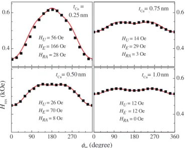
(2) PHYSICAL REVIEW B 75, 214402 共2007兲. 1. tCu = 0.25 nm. tCu = 0.25 nm. 0.6. tCu= .0.75 nm. 0.6. 0. -250. 0. 0. 180. MAG. (Oe). 90. Heb. Normalized magnetization. GESHEV et al.. HU = 56 Oe. HU = 14 Oe HE = 29 Oe HRA = 3 Oe. HE = 166 Oe. 0.4. -90. HRA = 28 Oe. 0.4. -1. φH (degree). tCu= .0.50 nm. FIG. 1. 共Color online兲 Left: In-plane magnetization curves for the sample with tCu = 0.25 nm for field along the easy 共circles兲 and hard 共triangles兲 directions; right: the corresponding HMAG angular eb variation 共diamonds兲. The lines are the best-fitting curves obtained using HU = 65 Oe, HW = 510 Oe, HE = 142 Oe, HRA = 14 Oe, ␴AF = 0.12 rad, and ␴FM = 0.10 rad.. In order to reproduce the rounded shape of the magnetization curves, one has to assume partly disordered interface moments by considering certain easy axis direction distributions 共with standard deviation ␴兲. Each exchange-coupled AF/FM pair was assumed to obey the model12,16 of Mauri et al., which has the FM uniaxial anisotropy field HU共=2K / M兲, the AF domain-wall anisotropy field HW关=␴W / 共tM兲兴, and the coupling field HE关=J / 共tM兲兴 as parameters. It is worth emphasizing that HE, an intrinsic property of the AF/FM system, is different from Heb which, in general, depends on J, HU, and HW.12 Here, t is the thickness of the Co layer, and M and K are its saturation magnetization and uniaxial anisotropy constant, respectively, J is the AF/FM coupling constant, and ␴W is the energy per unit surface of an AF domain wall. The calculations for the as-made sample with tCu = 0 nm have indicated that the AF part of the interface is almost fully spin compensated 共though disordered兲 and nearly uncompensated after annealing, and that the annealing improved the interfacial IrMn spin alignment without changing the Co anisotropy.14 Our fittings of the FMR data 共see below兲 showed that there is an additional field acting on the samples, i.e., the rotatable anisotropy field HRA 共=2KRA / M兲, a field that rotates to be parallel to the equilibrium direction of the FM magnetization and is responsible for the frequently observed resonance field shift.6 This originates from the unstable AF magnetic moments at the interface and can substantially change the shape of the magnetization curves and their characteristics.17 Here, we used HRA as an additional parameter in both magnetization and FMR simulations. The magnetic free energy per unit area can be written as E = − H · M + 2␲共M · n̂兲2 − K − ␴W. 共M · û兲2 共M · ĥ兲2 − K RA M2 M2. M · MAF MAF · ûAF −J , MM AF M AF. 共1兲. where the first four terms are the Zeeman, demagnetizing, FM uniaxial, and rotatable anisotropy energies, respectively. The last two terms are the AF domain-wall anisotropy and the AF/FM exchange coupling. The unit vectors û and ûAF. Hres (kOe). Magnetic Field (Oe). tCu= .1.0 nm. HU = 26 Oe HE = 70 Oe HRA = 8 Oe. 0. 90. 180. HU = 12 Oe HE = 12 Oe HRA = 0 Oe. 270. 0. 90. 180. 0.6. 0.4. 270. 360. φH (degree) FIG. 2. 共Color online兲 Angular variations of the resonance field for different tCu. Symbols represent the experimental data and the lines are calculated using the parameters given in each panel as well as HW = 510 Oe and M Co = 1372 emu/ cm3.. represent the FM and AF layers’ uniaxial anisotropy directions, respectively; n̂ and ĥ are the normal to the film surface and the applied field directions, respectively. The value of 1372 emu/ cm3 for M of Co, estimated from the fitting of Hres共␾H兲 for the film with tCu = 1.0 nm 共for which HRA = 0兲, was subsequently used in all simulations. In the latter, the normalized 共to their saturation values兲 magnetizations, i.e., the cosines of the angles between M 共and MAF兲 and H, are obtained by minimizing the energy given by Eq. 共1兲; details on the numerical procedure employed can be found in Refs. 12 and 13. The best-fitting magnetization curves for tCu = 0.25 nm are plotted in Fig. 1. Note that independent AF and FM easy axis distributions were used. There is very good agreement between model and experiment for both easy and hard direcMAG 共␾H兲, confirming that the tions, and the same holds for Heb magnetic behavior of such IrMn/ Co systems can be very well explained using coherent rotation models.18 Since the AF layers were first deposited, their intrinsic anisotropy should not change distinctly after the subsequent growth of the Cu layers independently of their thickness, so HW = 510 Oe was used for all tCu. Although easy axis distributions have been used in the magnetization curve calculations only, the same energy expression has been employed in both MAG and FMR simulations. The full squares in Fig. 2 represent the angular variations of the experimentally measured resonance fields. The lines in this figure give the corresponding best-fitting curves, calculated with the help of the previously derived13 关for the energy given by Eq. 共1兲兴 expression for Hres共␾H兲 and using the parameters given in each panel. It is worth noting that the above cited analytical expression depends not only on M, t, HU, HW, J, and ␻, but also on the equilibrium angles of M and MAF. Here, these angles were estimated using the same numerical procedure as that employed in the magnetization curve fittings obtained in the present work.. 214402-2.

(3) PHYSICAL REVIEW B 75, 214402 共2007兲. 30. J. 90. 0.10. FMR. ∆H (Oe). EXCHANGE BIAS THROUGH A Cu INTERLAYER IN AN…. -90 Heb (Oe). tCu= 0.25 nm. tCu= 0.75 nm. 0.05 0. tCu= 1.0 nm. tCu= 0.50 nm 45. 90. 135. 0. 45. 90. 135. 1. 1. 50. FIG. 3. 共Color online兲 Experimental angular variations of HFMR eb 共full squares兲 and of HMAG 共empty circles兲. eb. The significant difference between the Hres共␾H兲 curve for tCu = 0.25 nm and the others plotted in Fig. 2 indicates that when tCu increases, the coupling strength decreases and the Hres共␾H兲 curves become typical of the case when HU ⬍ HE Ⰶ HW.13 The quite good coincidence between model and experiment confirms the above observations. For HE ⫽ 0, the EB field obtained from FMR measureFMR ments has been defined13 as Heb 共␾H兲 = 21 关Hres共␾H兲 − Hres共␲ + ␾H兲兴 and, like Hres, strongly depends on the interaction strength. For high HE / HW ratios, its angular depenMAG ; they may, howdence becomes very close to that of Heb ever, show rather different variations in the case of weak interactions 共i.e., when HE Ⰶ HW兲, depending on the HU value as well. FMR versus ␾H, obtained using the measured Hres共␾H兲 Heb fields from Fig. 2, are plotted in Fig. 3 along with the experiMAG angular variations. Different from the data remental Heb ported in the literature until now,4–11 these “field shifts,” obtained from different measurement techniques, coincide. The FMR MAG and Heb is expected13 for HE rather overlap between Heb higher than HU. Although such a coincidence is observed also for the other samples, one cannot conclude that they are strongly coupled from the analysis of their experimental curves only. The reason is that the error margin in the estimation, from the experiments, of both kinds of Heb fields could be of the order of the difference between them when HE and HU are comparable in value. The Heb共␾H兲 curves for the film with the thickest Cu spacer shown in Fig. 3 are exactly what one would expect for FMR shows almost a very weakly coupled bilayer: while Heb MAG pure sin 2␾H variation, Heb deviates from the sine behavior in the vicinities of ␾H = 0 and ␲, as exemplified in Fig. 2共a兲 of Ref. 13. Figure 4 shows the variations of J 共=tMHE兲, HU, and FMR HRA vs tCu, obtained from the fittings. Both JFMR and JMAG decrease exponentially for tCu 艌 0.25 nm, i.e., J ⬀ exp共−tCu / ␭兲, when tCu increases. The decay lengths ␭ are estimated to be ␭FMR ⬇ 2.9 Å and ␭MAG ⬇ 3.1 Å, values. σAF σFM. 0. FMR. tCu (nm). 1. HRA 0 0.00. φH (degree). HU. 0. -10 180. HU. FMR. σ (rad). HU , HRA (Oe). 0. -50. tCu (nm). 0.0 MAG. 0. 0. MAG. -30 10. 50. J. 2. 0. 0. J (erg/cm ). 0.1. 0.25. 0.50. tCu (nm). 0.75. 1.00. FIG. 4. 共Color online兲 Spacer thickness dependencies of J, HU, and HFMR RA as estimated by fitting the FMR and magnetization data. The FMR linewidth variation is plotted in the top-panel inset, and the bottom-panel inset shows the AF and FM easy axis distributions used in the magnetization curve fittings. The solid J共tCu兲 curves are best-fit results to exponential decay; all other curves are guides for the eyes.. rather smaller than those reported by Gökemeijer et al.2 and comparable with those of Thomas et al.3 The short ␭ of a few angstroms indicates the so-called “short-range” coupling. The correct term, however, should be direct coupling, since it is, most probably, due to direct interfacial AF/FM contact through pinholes between the IrMn and Co layers, which normally occurs up to insertion layer thickness of ⬇1 nm.3,20,21 As tCu gets thicker, the number of pinholes and their surface decrease and so does the effective coupling strength. HU and HRA, however, after rapid initial decrease with tCu, remain almost constant for tCu 艌 0.75 nm. Remarkably, FMR MAG ⬍ HU for all tCu. JFMR ⬎ JMAG and HU The thickness dependence of J and the anisotropy parameters of our samples are consistent with the following scenario. Let us start with the Co layer characteristics. Although both AF and FM layers are polycrystalline, the Co layer spin alignment is improved when increasing the thickness of the bottom-grown Cu layer due to the improvement of its crystallographic structure. This is corroborated by the gradual decreases with tCu of the FM easy axis distribution estimated from the magnetization curve simulations, ␴FM, shown in Fig. 4 and of the FMR linewidth, ⌬H, also plotted in this figure. In polycrystalline materials, ⌬H is increased because the dispersion in the anisotropy parameters 共due to, e.g., interface roughness, defects, etc.兲 causes separate magnetic regions to resonate at different applied fields. Part of the ⌬H decrease could also be attributed to the weakening of the coupling strength.22 Furthermore, ⌬H could be interface dependent.23 Contrary to the FM spin arrangement variation, the AF moment alignment becomes worse when tCu is increased, as indicated by the ␴AF共tCu兲 curve in Fig. 4. The increase of ␴AF with tCu at first sight may seem strange, since the IrMn layers. 214402-3.

(4) PHYSICAL REVIEW B 75, 214402 共2007兲. GESHEV et al.. are deposited before the Cu ones. However, this increase is naturally explained, having in mind that the interfacial AF spins are not coupled directly to the field but to the FM magnetization. The AF/FM contact area decreases as the Cu layer gets thicker due to the decrease of the number and the surface of the pinholes, and so does the number of the AF spins possible to be aligned. Thus, the capability of magnetic annealing to form an AF collinear arrangement gradually decreases, despite the fact that IrMn is a cubic anisotropy material with four easy magnetization axes, i.e., with good potential for improving its spin alignment. There are two coexisting fractions of grains at the AF part of the interface: magnetically stable and unstable AF grains.24 In EB systems, the stability is predominantly determined by the coupling strength between these grains’ moments and the adjacent FM domains. In FMR experiments, whether a magnetic moment is stable or not depends on its relaxation time ␶ relative to the period of the microwave excitation, ␶res. It has been shown19 that the exchange bias could be frequency dependent, i.e., Hres共␾H兲 obtained at two different excitation frequencies on the same piece of sample could differ considerably, the curve being obtained at lower ␻ characteristic of strong exchange coupling and that measured at higher ␻ typical of weak interactions. The reason is that only grains with ␶ ⬎ ␶res contribute to the exchange bias. Some of the moments which are stable in an FMR measurement are unstable in a magnetization curve trace, since the measurement time of the latter is longer than ␶, thus explaining the effectively lower JMAG value as compared to that extracted from the FMR technique. AF grains with ␶ ⬇ ␶res contribute to the rotatable anisotropy and not to the exchange bias in FMR measurement.6,24 FMR MAG Here, HRA = 2HRA was used in the simulations for all samples, the cause being, once again, that responsible for JFMR ⬎ JMAG: due to their low ␶ values, some of the moments FMR are “sensed” as superparamagnetic in that contribute to HRA a dc magnetization measurement.. W. H. Meiklejohn and C. P. Bean, Phys. Rev. 102, 1413 共1956兲; 105, 904 共1957兲. 2 N. J. Gökemeijer, T. Ambrose, and C. L. Chien, Phys. Rev. Lett. 79, 4270 共1997兲. 3 L. Thomas, A. J. Kellock, and S. S. P. Parkin, J. Appl. Phys. 87, 5061 共2000兲. 4 B. H. Miller and E. Dan Dahlberg, Appl. Phys. Lett. 69, 3932 共1996兲. 5 V. Ström, B. J. Jönsson, and E. D. Dahlberg, J. Appl. Phys. 81, 5003 共1997兲. 6 R. D. McMichael, M. D. Stiles, P. J. Chen, and W. F. Egelhoff, Jr., Phys. Rev. B 58, 8605 共1998兲. 7 E. D. Dahlberg, B. Miller, B. Hill, B. J. Jönsson, V. Ström, K. V. Rao, J. Nogués, and Ivan K. Schuller, J. Appl. Phys. 83, 6893 共1998兲. 8 P. Miltényi, M. Gruyters, G. Güntherodt, J. Nogués, and Ivan K. Schuller, Phys. Rev. B 59, 3333 共1999兲. 9 H. Xi, R. M. White, and S. M. Rezende, Phys. Rev. B 60, 14837 共1999兲. 1. Both FMR and magnetization techniques show that HU rapidly increases with the decrease of tCu starting from tCu ⬇ 0.75 nm. It remains approximately constant for higher Cu thicknesses, where J ⬇ 0, which clearly indicates that the increase of HU is an exchange-induced effect. This could be attributed to a presence of AF/FM subsystems with incompletely compensated AF interface along the effective easy axis of the sample, which results in an enhanced width of the hysteresis loops.25 In the framework of our model, which does not account for configurations of the type where a FM moment is coupled to two AF sublattice moments, this enhancement is interpreted as an additional contribution to HU. Since J becomes weaker with the increase of tCu, the role of this three-moment system decreases and, consequently, so does HU. The above considerations also explain the lower values of HU estimated from FMR data as compared to those extracted from the magnetization curve fittings. Some of the AF grains with ␶ ⬎ ␶res, although stable for FMR and contributing to the FMR . They, however, EB, do not give an additional raise to HU contribute to HU in the “slower” magnetization measurements. In summary, we observed identical exchange-bias fields and different coupling strengths and anisotropy fields, obtained via FMR and magnetization measurements, when the direct coupling through pinholes in the Cu interlayer is not negligible in our IrMn/ Cu/ Co system. These features were attributed to magnetic layers with independent easy axis distributions, to the distinct measurement times of the techniques, and to the role of AF grains with different sizes and different magnetic stabilities at the AF side of the interface. ACKNOWLEDGMENT. This work has been supported by the Brazilian agencies CNPq, FAPERGS, and CAPES.. 10. J. R. Fermin, M. A. Lucena, A. Azevedo, F. M. de Aguiar, and S. M. Rezende, J. Appl. Phys. 87, 6421 共2000兲. 11 R. L. Rodríguez-Suárez, L. H. Vilela Leão, F. M. de Aguiar, S. M. Rezende, and A. Azevedo, J. Appl. Phys. 94, 4544 共2003兲. 12 J. Geshev, Phys. Rev. B 62, 5627 共2000兲. 13 J. Geshev, L. G. Pereira, and J. E. Schmidt, Phys. Rev. B 64, 184411 共2001兲. 14 S. Nicolodi, L. C. C. M. Nagamine, A. D. C. Viegas, J. E. Schmidt, L. G. Pereira, C. Deranlot, F. Petroff, and J. Geshev, J. Magn. Magn. Mater. 共to be published兲. 15 S. Nicolodi, L. G. Pereira, J. E. Schmidt, L. C. C. M. Nagamine, A. D. C. Viegas, C. Deranlot, F. Petroff, and J. Geshev, Physica B 384, 141 共2006兲. 16 D. Mauri, H. C. Siegmann, P. S. Bagus, and E. Kay, J. Appl. Phys. 62, 3047 共1987兲. 17 J. Geshev, L. G. Pereira, and J. E. Schmidt, Phys. Rev. B 66, 134432 共2002兲. 18 J. Camarero, J. Sort, A. Hoffmann, J. M. García-Martín, B. Dieny, R. Miranda, and J. Nogués, Phys. Rev. Lett. 95, 057204. 214402-4.

(5) PHYSICAL REVIEW B 75, 214402 共2007兲. EXCHANGE BIAS THROUGH A Cu INTERLAYER IN AN… 共2005兲. J. Geshev, L. G. Pereira, J. E. Schmidt, L. C. C. M. Nagamine, E. B. Saitovitch, and F. Pelegrini, Phys. Rev. B 67, 132401 共2003兲. 20 Y. G. Yoo, S. G. Min, and S. C. Yu, J. Magn. Magn. Mater. 304, e718 共2006兲. 21 J. Wang, J. Appl. Phys. 91, 7236 共2002兲. 22 R. D. McMichael, M. D. Stiles, P. J. Chen, and W. F. Egelhoff, Jr., J. Appl. Phys. 83, 7037 共1998兲. 19. 23 S.. Mizukami, Y. Ando, and T. Miyazaki, Phys. Rev. B 66, 104413 共2002兲. 24 E. Fulcomer and S. H. Charap, J. Appl. Phys. 43, 4190 共1972兲; M. D. Stiles and R. D. McMichael, Phys. Rev. B 59, 3722 共1999兲; 63, 064405 共2001兲. 25 R. E. Camley, B. V. McGrath, R. J. Astalos, R. L. Stamps, JooVon Kim, and Leonard Wee, J. Vac. Sci. Technol. A 17, 1335 共1999兲.. 214402-5.

(6)