TítuloIber applications basic guide: Two dimensional modelling of free surface shallow water flows

Texto completo

(1)Iber applications basic guide. Two-dimensional modelling of free surface shallow water flows www.iberaula.es. Luis Cea Gómez Ernest Bladé i Castellet Marcos Sanz Ramos María Bermúdez Pita Ángel Mateos Alonso.

(2)

(3) Iber applications basic guide Two-dimensional modelling of free surface shallow water flows. Luis Cea Gómez Ernest Bladé i Castellet Marcos Sanz Ramos María Bermúdez Pita Ángel Mateos Alonso. A Coruña 2019. Servizo de Publicacións Universidade da Coruña.

(4) Iber applications basic guide. Two-dimensional modelling of free surface shallow water flows CEA GÓMEZ, Luis (https://orcid.org/0000-0002-3920-0478) BLADÉ I CASTELLET, Ernest (https://orcid.org/0000-0003-1770-3960) SANZ RAMOS, Marcos (https://orcid.org/0000-0003-2534-0039) BERMÚDEZ PITA, María (https://orcid.org/0000-0003-3189-4791) MATEOS ALONSO, Ángel A Coruña, 2019 University of A Coruna Press Number of pages: 105 Contents, pages: 5-7 DOI: https://doi.org/10.17979/spudc.9788497497176 ISBN: 978-84-9749-717-6 Dep. legal: C 822-2019 CDU: [519.62:004.4][556.53/.54:627.13](035)*IBER IBIC: TNF | UM | 4GE. EDITION University of A Coruna Press Universidade da Coruña, Servizo de Publicacións <http://www.udc.gal/publicacions> © edition, Universidade da Coruña (University of A Coruna) © contents, authors. This book is released under a Creative Commons license Attribution-NonCommercial-ShareAlike (CC BY-NC-SA) 4.0 International.

(5) Iber Applications Basic Guide. Contents 1. INTRODUCTION.............................................................................................. 9 2. IBER......................................................................................................... 11 3. PRACTICAL EXAMPLE 1: STREET INTERSECTION ........................................................ 12 3.1. Objectives .............................................................................................. 12 3.2. Description of the case study and input data ........................................................ 12 3.3. Model set-up ........................................................................................... 14 3.3.1. Geometry .......................................................................................... 14 3.3.2. Hydrodynamics .................................................................................... 16 3.3.3. Mesh ............................................................................................... 17 3.3.4. Calculation data ................................................................................... 19 3.3.5. Calculation process ................................................................................ 19 3.4. Results .................................................................................................. 20 3.5. Conclusions ............................................................................................. 24 3.6. References .............................................................................................. 24 4. PRACTICAL EXAMPLE 2: RIVER FLOOD INUNDATION................................................... 25 4.1. Objectives .............................................................................................. 25 4.2. Description of the case study and input data ........................................................ 25 4.3. Model set-up ........................................................................................... 26 4.3.1. Geometry .......................................................................................... 26 4.3.2. Hydrodynamics .................................................................................... 29 4.3.3. Mesh ............................................................................................... 32 4.3.4. Calculation data ................................................................................... 34 4.3.5. Calculation process ................................................................................ 35 4.4. Results .................................................................................................. 35 4.5. Conclusions ............................................................................................. 40 4.6. References .............................................................................................. 40 5. PRACTICAL EXAMPLE 3: BRIDGES AND CULVERTS ...................................................... 41 5.1. Objectives .............................................................................................. 41 5.2. Description of the case study and input data ........................................................ 41 5.3. Model set-up ........................................................................................... 41.

(6) Iber Applications Basic Guide. 5.3.1. Geometry .......................................................................................... 41 5.3.2. Hydrodynamics .................................................................................... 45 5.3.3. Culverts............................................................................................. 46 5.3.4. Bridges ............................................................................................. 48 5.3.5. Mesh ............................................................................................... 48 5.3.6. Calculation data ................................................................................... 49 5.3.7. Calculation process ................................................................................ 49 5.4. Results .................................................................................................. 50 5.4.1. Hydrodynamic results ............................................................................. 50 5.4.2. Bridge results ...................................................................................... 51 5.4.3. Culver results ...................................................................................... 52 5.5. Conclusions ............................................................................................. 53 5.6. References .............................................................................................. 54 6. PRACTICAL EXAMPLE 4: DAM BREAK .................................................................... 55 6.1. Objectives .............................................................................................. 55 6.2. Description of the case study and input data ........................................................ 55 6.3. Model set-up ........................................................................................... 56 6.3.1. Geometry .......................................................................................... 56 6.3.2. Hydrodynamics .................................................................................... 57 6.3.3. Mesh ............................................................................................... 58 6.3.4. Breach .............................................................................................. 58 6.3.5. Calculation data ................................................................................... 60 6.3.6. Calculation process ................................................................................ 61 6.4. Results .................................................................................................. 61 6.4.1. Hydrodynamic results ............................................................................. 61 6.4.2. Dam break results ................................................................................. 63 6.5. Conclusions ............................................................................................. 65 6.6. References .............................................................................................. 65 7. PRACTICAL EXAMPLE 5: SEDIMENT TRANSPORT: BEDLOAD ........................................... 67 7.1. Objectives .............................................................................................. 67 7.2. Description of the case study and input data ........................................................ 67 7.3. Model set-up ........................................................................................... 68 7.3.1. Geometry .......................................................................................... 68 7.3.2. Hydrodynamics .................................................................................... 68.

(7) Iber Applications Basic Guide. 7.3.3. Mesh ............................................................................................... 70 7.3.4. Sediment transport ................................................................................ 71 7.3.5. Calculation data ................................................................................... 71 7.4. Results .................................................................................................. 73 7.5. Conclusions ............................................................................................. 79 7.6. References .............................................................................................. 80 8. PRACTICAL EXAMPLE 6: WASTEWATER DISCHARGE OF CBOD AND AMMONIA IN A RIVER ........ 81 8.1. Objectives .............................................................................................. 81 8.2. Description of the case study and input data ........................................................ 81 8.3. Model set-up ........................................................................................... 83 8.3.1. Geometry .......................................................................................... 83 8.3.2. Hydrodynamics .................................................................................... 83 8.3.3. Water quality ...................................................................................... 84 8.3.4. Mesh ............................................................................................... 86 8.3.5. Calculation data ................................................................................... 86 8.4. Results .................................................................................................. 88 8.4.1. Initial checks ....................................................................................... 88 8.4.2. Hydrodynamic results ............................................................................. 89 8.4.3. Water quality results .............................................................................. 89 8.5. Conclusions ............................................................................................. 91 8.6. References .............................................................................................. 91 9. PRACTICAL EXAMPLE 7: SEWAGE SPILL IN AN ESTUARY ............................................... 93 9.1. Objectives .............................................................................................. 93 9.2. Description of the case study and input data ........................................................ 93 9.3. Model set-up ........................................................................................... 94 9.3.1. Geometry .......................................................................................... 94 9.3.2. Hydrodynamics .................................................................................... 96 9.3.3. Water quality ...................................................................................... 97 9.3.4. Mesh ............................................................................................... 99 9.3.5. Calculation data ................................................................................. 100 9.4. Results ................................................................................................ 101 9.5. Conclusions ........................................................................................... 104 9.6. References ............................................................................................ 104.

(8)

(9) Iber Applications Basic Guide. 1. Introduction This is a basic tutorial of Iber, aimed at new users who want to acquire a basic knowledge of the software. It is not intended to cover all the software’s capabilities, but rather to give a flavour of the typical applications of Iber and its main elements, so that new users can evaluate whether the software is appropriate for their needs. The basic steps to set up a computation from scratch are described in detail in each chapter, as well as the input data needed to run the model. The case studies described include Iber’s hydraulic, sediment transport, and water quality modules. Details about the equations and models implemented in Iber are not given in this document. Such information can be found in the Iber’s Hydraulic Reference Manual, as well as in Bladé et al. (2014), in Cea and Bladé (2015), in Cea et al. (2016), and in the references contained in those documents. Specific examples included in this document are the following:       . Practical Example 1 – Street intersection Practical Example 2 – River flood inundation Practical Example 3 – Bridges and culverts Practical Example 4 – Dam break Practical Example 5 – Sediment transport: bedload Practical Example 6 – Wastewater discharge of CBOD and ammonia in a river Practical Example 7 – Sewage spill in an estuary. Some examples need some digital input data to be completed, as Digital Elevation Models, ortophotos, or boundary conditions. These data is supplied together with this tutorial, and can also be retrieved from the model’s webpage. Further basic and advanced training of Iber is given via the Iber online courses (www.ibercursos.com) Model references Bladé, E., Cea, L., Corestein, G., Escolano, E., Puertas, J., Vázquez-Cendón, E., Dolz, J., Coll, A. (2014a). Iber: herramienta de simulación numérica del flujo en ríos. Revista Internacional de Métodos Numéricos para Cálculo y Diseño en Ingeniería, Volume 30, Issue 1, 2014, Pages 1-10, ISSN 02131315, DOI: 10.1016/j.rimni.2012.07.004 Cea, L., and Bladé, E. (2015). A simple and efficient unstructured finite volume scheme for solving the shallow water equations in overland flow applications. Water Resources Research, 51, 5464-5486. DOI: 10.1002/2014WR01654 Cea, L., Bermudez, M., Puertas, J., Blade, E., Corestein, G., Escolano, E., Conde, A., Bockelmann-Evans, B., and Ahmadian, R. (2016). IberWQ: new simulation tool for 2D water quality modelling in rivers and shallow estuaries. Journal of Hydroinformatics 18, 816–830. DOI: 10.2166/hydro.2016.235. 9.

(10)

(11) Iber Applications Basic Guide. 2. Iber Iber is a software package for simulating unsteady free-surface turbulent flow and transport processes in shallow water flows. The hydrodynamic module of Iber calculates the depth-averaged twodimensional shallow water equations (2D Saint-Venant Equations). A turbulent module allows the user to include the effect of the turbulent stresses in the hydrodynamics. These are evaluated with different depth-averaged turbulence models for shallow waters of different complexity. Additional capabilities include sediment transport modelling, water quality modelling, and rainfall-runoff modelling. All the equations of the model are provided in a finite-volume non-structured mesh made up of triangle and quadrilateral elements. A more detailed description of the model can be found in Bladé et al. (2014), Cea and Bladé (2015), Cea et al. (2016), and in the references contained in those documents. Other references, journal publications, congress proceedings and BSc, MSc and PhD theses can be found in the model’s webpage.. Learn more about Iber and download it for free:. www.iberaula.com Have a look to our high-level and quality online and classroom trainings:. www.ibercursos.com. 11.

(12) Iber Applications Basic Guide. 3. Practical Example 1: Street intersection 3.1. Objectives This chapter introduces the Iber interface (GiD) and the basic aspects of the hydrodynamic module. It illustrates the basic tools for creating and editing the geometry of a model. Using a street intersection example, we will see elements related to the definition of the geometrical properties and the importance of these regarding the mesh generation process. This exercise will also serve to illustrate the importance of a 2D model as a means of accurately reproducing certain hydraulic phenomena, such as hydraulic jumps and crossed waves.. 3.2. Description of the case study and input data The example consists of two perpendicular channels that represent two scaled streets with different slopes. The streets intersect on a horizontal surface (Figure 1).. Figure 1. Representation of the street intersection. This example is a laboratory case study used to analyse the flow distribution between two streets (Nanía Escobar, 1999) and to validate Iber’s hydrodynamic module (Bladé, 2005). The area under study involves three flow regimes (supercritical, critical and subcritical) due to the different slopes of the streets. A hydraulic jump is formed in the intersection area. The geometry is detailed in Table 1. Please note that all units used in Iber are defined in the International System Units (SI). Coordinates are in metres.. 12.

(13) Iber Applications Basic Guide. Table 1. Geometric description of the streets (coordinates in meters). Point 1 2 3 4 5 6 7 8 9 10 11 12 13 14 15 16. X 0 0 1.5 1.5 -1.5 -1.5 0 1.5 3 6.3 3 6.3 0 1.5 0 1.5. Y 0 1.5 0 1.5 0 1.5 3 3 0 0 1.5 1.5 -1.5 -1.5 -4.8 -4.8. Z 0 0 0 0 0.015 0.015 0.03 0.03 -0.015 -0.05 -0.015 -0.05 -0.03 -0.03 -0.1 -0.1. The two streets are oriented by X and Y Cartesian directions, and each street has a different inlet discharge and slope (Figure 2).. 1.5 m. 1.5 m. 3.3 m. 1.5 m. 7. 8. 2. 4. 11. 1. 3. 9. 13. 14. 15. 16. 1.5 m. 6. 12. 1.5 m. 5 1.5 m. 3.3 m. Figure 2. Schematic representation of the model.. 13. 10.

(14) Iber Applications Basic Guide. 3.3. Model set-up 3.3.1. Geometry The first step when starting a new simulation from scratch is to save the model (Files>>Save).. Figure 3. Save project window. The geometry of the model will be generated with squares and rectangles (Figure 2). Using points, lines and surfaces we will obtain the complete geometry of the streets. First, we introduce the coordinates of the points that define the intersection area, using Geometry>>Create>>Point (points 1 to 4). On the Command line (located at the bottom of the interface) we insert the coordinates of point 1 (Table 1). Once the coordinates of point 1 have been introduced, we press ESC, and we repeat this procedure for points 2, 3 and 4 1. We then join these points with lines. Using Geometry>>Create>>Straight line, we click on point 1. The Create point procedure window (Figure 4) will appear. We want to use an already existing point (number 1) as the first point of the line, so we click Join.. Figure 4. Creation point procedure window.. 1. Note that the format of the coordinate system is “a,b,c”, where a, b and c represents the values of the coordinates X, Y and Z, respectively. The comma is the coordinate separator, and the decimal separator is based on SI (point).. 14.

(15) Iber Applications Basic Guide. We repeat this action to create the other lines (2-4, 3-4, 1-3) and press ESC to end this action. Finally, we create a NURBS surface 2, using the By Contour option in the Geometry>>Create>>NURBS Surface menu. Select all the lines and press ESC. The result of those operations is shown in Figure 5 3.. Figure 5. Surface created. With Geometry>>Create>>Straight line we can now create the lines 1-5, 5-6 and 2-6 using the coordinates shown in Table 1 directly. Note that when we create the lines, Iber asks if we want to use an already existing point (Join option). Once the lines are created, we need to create a surface defined by these lines that form a closed polygon. We turn now to the Copy menu (Utilities>>Copy). This allows us to perform different kinds of operations. In this case, we are going to copy line 2-4 in order to generate lines 2-7 and 4-8. In Entities type we choose Select lines. The first point is point number 2 and the end point is point number 7 (see coordinates on Table 1). Click on Select and choose line 2-4. Then press ESC or click Finish. Join points 27 and 4-8 with their respective lines. Finally, we can create the surface. Using the Copy tool, we can create new lines and the surfaces within them using the Do Extrude option. Following the steps previously described, we generate line 9-11 using line 3-4 and line 4-11 using line 39. The surface will be created automatically. Copy line 3-4 from point 3 to 9, and in the Do Extrude option choose Surface. Select the translation as operation, insert the first and the second points, then select the line (3-4). Press ESC to finish. Repeat this action with line 9-11 to create lines 10-12, 9-10 and 11-12 and the corresponding surface. Do the same with line 1-3 and then with line 13-14. The result of all operations is shown in Figure 6.. 2. Non-Uniform Rational Basis-Splines are the kind of shapes used by GiD to represent the surfaces. 3 GiD represents the geometry of the model by points, lines and surfaces. By default, points are coloured black, lines are dark blue, and surfaces are purple. The surface representation has a smaller shape than the closed polygon that encloses it.. 15.

(16) Iber Applications Basic Guide. Figure 6. Geometry of the model.. 3.3.2. Hydrodynamics The next step is to assign the hydrodynamics boundary and initial conditions. The model has two inlets and two outlets (which must be defined as boundary conditions). The simulation starts with the streets being dry (initial condition). All the hydrodynamics conditions are defined in the Data menu. Boundary conditions are assigned in Data>>Hydrodynamics>>Boundary conditions. A constant discharge of 0.04286 m3/s on line 5-6 will be assigned using the 2D Analysis window (Figure 7). In the Inlet field we choose Total Discharge. In the Inlet Condition field we choose the Critical/Subcritical regime. In Total Discharge we expand the table ( ) and introduce a unique value of discharge at the 4 time 0 seconds . Introduce the value “0.04286” in the “Q [m3/s]” column and Assign this condition to the line 5-6. The Inlet Num is 1. Repeat this action with line 7-8, but here the inlet is defined by a Specific Discharge and Supercritical Flow Regime. The value of this boundary condition is a specific discharge of 0.0667 m2/s and a water elevation of 0.0771 m, corresponding to a discharge of 0.1 m3/s.. 4. A constant value is introduced in Iber from time ti to tf. If the simulation time is greater than tf, Iber considers this value to be constant from tf. to the end of the simulation.. 16.

(17) Iber Applications Basic Guide. Figure 7. 2D Analysis window. Characteristics of the inlets on line 5-6 (left) and on line 7-8 (right). The characteristics of the laboratory experiment produce a mixed regime flow (subcritical and supercritical). The outlet conditions of lines 10-12 and 15-16 are supercritical flow (Froude number greater than 1). We use the drop-down menu to change between Inlet and Outlet conditions. Note that the Outlet Num must be 1 and 2, respectively. As mentioned previously, the initial condition is a dry channel, meaning that water depth is zero. Thus, using Data>>Hydrodynamics>>Initial condition we assign a water depth equal to zero to all surfaces. Finally, the model needs a roughness coefficient. We define this in Data>>Roughness>>Land use (Figure 8). Iber has a database of land uses with common Manning roughness coefficient values. Use the dropdown menu and choose Concrete, which has a Manning value of 0.018 s·m-1/3. Assign this to all surfaces and press ESC.. Figure 8. Land Use window, where the Manning coefficient is defined.. 3.3.3. Mesh The mesh is the discretization of the space domain where Iber solves the Shallow Water Equations (SWE). Iber can work with structured and non-structured meshes with triangular or/and quadrilateral elements. Mesh options are defined from the Mesh menu. In this example, we will use a structured grid formed by quadrilateral elements. Using Mesh>>Structured>>Surfaces>>Assign size we define the size of the mesh elements. In this case, all elements will have the same length. Select all surfaces and press ESC. A new window will ask for the 17.

(18) Iber Applications Basic Guide. elements size. Introduce 0.1 metres and then select Assign to all the lines. Press ESC and close the window. We now generate the mesh (Mesh>>Generate mesh). The Mesh Generation window asks for an element size. We have already defined this, so the value introduced here will not be taken into account. Press OK.. Figure 9. Progress in the Meshing window, in which some properties of the created mesh are shown. The Progress in meshing window automatically appears (Figure 9). This window shows the number and kind of elements generated (triangular or quadrilateral), the number of nodes, and the memory used in this process. In this case a mesh of 2115 quadrilateral elements has been created. We can view the mesh by clicking on View Mesh (Figure 10).. 18.

(19) Iber Applications Basic Guide. Figure 10. View of the mesh of the model.. 3.3.4. Calculation data The Data settings define the general and numerical parameters of the simulation (time, results, calculation modules, etc.).. Figure 11. Data window. Time parameters tab. In this example we only need to define the Time Parameters, using Data>>Problem data. We start the simulation at a time equal to zero seconds (Initial time) and finish it at 35 seconds (Max simulation time). We want results to be saved every second, so we define the Result time interval as 1 (Figure 11). Press Accept to save these parameters.. 3.3.5. Calculation process We have already built the model, and now we need to calculate it. Through Calculate>>Calculate we can begin the simulation. When the calculation process has finished, the Process info window will appear (Figure 12). Press OK to maintain the preprocess interface or press Postprocess to see the results.. Figure 12. Process info window. It is possible to toggle between pre- and postprocess view using the File menu or the. button.. Before we view the results, we will check if the simulation process has been successful. In the View process info window (Calculate>>View process info window), Iber shows some information about the calculation process (name of the project, time starting, Iber version, etc.). This window also shows warnings and error messages. These alert the user to any issues that have occurred during the computation process (e.g. a missed condition, problems with the mesh, a duplicated boundary condition, non-permitted boundaries or internal conditions, etc.). 19.

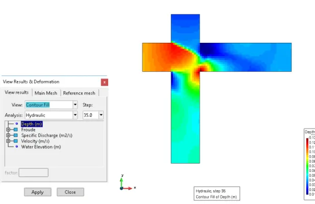
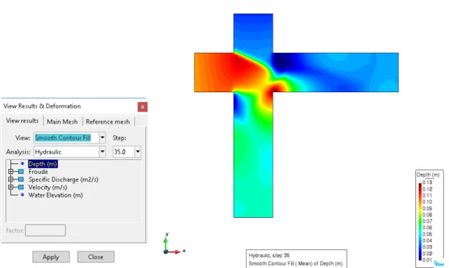
(20) Iber Applications Basic Guide. If the computation has been performed successfully, the message COMPUTATION FINISHED SUCCESSFULLY! will appear at the bottom of the View process info window, along with the data and the time when it finished.. 3.4. Results In Window>>View results we can choose the different ways to show the results (Figure 13). We will represent the depth field at the last time calculated (35 seconds). Select Contour fill in View, Hydraulic in Analysis, 35 in Step, then Depth as the result to show. Press Apply and the results will be drawn on the elements (Figure 13).. Figure 13. Contour fill representation of the depth result at 35 seconds. Contour fill represents the results using one colour on each element. If we want to represent a “nonpixelated” representation, we can use the Smooth Contour fill View (Figure 14). We can observe upstream of the intersection that on the X-oriented street the water depth is greater than on the Y-oriented street. In the intersection the two flows converge, forming a hydraulic jump. Crossed waves are then generated on the X and Y streets downstream of the confluence. In order to reach a better representation of the hydraulic jump, we can represent the Froude number. A hydraulic jump is generated when a flow changes its hydraulic regime from supercritical (Froude less than 1) to subcritical (Froude greater than 1). Select the Froude module (|Froude|) result in the Hydraulic Analysis as a Smooth Contour fill, View at 35 s, and Apply. We can see that X-street has a subcritical flow (dark blue on Figure 15 left) and Y-street has a supercritical flow (dark red on Figure 15 left). 20.

(21) Iber Applications Basic Guide. Figure 14. Smooth Contour fill representation of the depth result at 35 seconds.. Figure 15. Froude number representation. Smooth Contour fill representation of the Froude value at 35 seconds (left) and Smooth Contour fill representation of the Froude value limited to 1 at 35 seconds (right). We can set the maximum and minimum values to be shown using Utilities>>Set contour limits>>Define limits (Figure 16). Set the maximum value to 1, and Apply. In Figure 15 (right) we can see the subcritical 21.

(22) Iber Applications Basic Guide. flow in colours and the supercritical flow as black colour. To finish this result representation, unmark “Max” and then apply, or using Utilities>>Set contour limits>>Reset limits menu.. Figure 16. Contour Limits window. Maximum value fixed at “1”. Another common way of representing results is by using Vectors. This is only available for vector variables as specific discharge and velocity. Using the View Results & Deformation window (View results tab), select Display Vectors View, the velocity module (|Velocity|) at the last time step (35 s), and Factor equal to 1. Select Apply. The velocity is shown as multicolour arrows, but they are overlapping (Figure 17 left). We can modify the details of the representation using Utilities>>Preference. First, open the Postprocess>Vectors options and select Monochrome as Colour mode, then change Vector size type to Fixed, and then apply. The results of these operations are shown in Figure 17 (right).. Figure 17. Vector representation of the velocity module. With this representation we can observe a recirculation area on Y-street, downstream of the street intersection. We can also observe that the discharge on the Y-street is greater than on the X-street. If we represent the two components of the velocity we see that, in general, the Y component is greater than the X component (Figure 18). Another kind of available results are graphical representation by Graphs, which can be used to represent the time evolution of a variable, and to create cross sections or hydrographs using the Window>>View graphs options. 22.

(23) Iber Applications Basic Guide. Figure 18. Vector representation of the X (left) and Y (right) velocity. We start by plotting the time evolution of the water elevation at the control point located in the middle of the intersection area ([0.75,0.75]). On the Create tab we select Point evolution View, hydraulic Analysis and any time step (for the present example, this parameter is not needed). On the X-axis (for All steps) of the graph we do not select anything, and for the Y-axis we choose Water Elevation. After we select Apply, Iber asks for the coordinates of the point. Introduce “0.75,0.75” in the Command line (at the bottom of the interface) and press Finish or ESC (Figure 19). It might also be of interest to show the water level at a specific time step. In this case, the last time step simulated represents a steady state situation. We will create another graph-set here, using the button Create ( ). In the Create tab select Line Graph View of the Water elevation at step 35 s. Select Line Variation and Water Elevation for the X-axis and the Y-axis respectively. Select Apply and indicate the line which serves to plot the water surface. The first point is [0.75,3] and the last point is [0.75,-4.8]. In the same graph we will plot the bottom elevation. We follow the same steps, but changing the Analysis to Topography, the Step to “0”, and the Y-axis value to Elevation. The result is shown in Figure 20.. Figure 19. Graph of the water elevation evolution in time. 23.

(24) Iber Applications Basic Guide. Figure 20. Graph of the water elevation along the Y-direction.. 3.5. Conclusions In this example we have introduced the user to the Iber’s interface. The basic tools and geometry options have been shown by creating a simple model. It has also been shown how to introduce the basic flow conditions (boundary and initial conditions, roughness, etc.). A structured mesh criteria has been used to discretize the spatial domain. The results show a hydraulic jump and crossed waves, characteristic of a 2D shallow water flow.. 3.6. References Bladé, E. (2005). Modelación del flujo en lámina libre sobre cauces naturales análisis integrado con esquemas en volúmenes finitos en una y dos dimensiones. Tesis Doctoral. Universitat Politècnica de Catalunya. Retrieved from http://tesisenred.net/handle/10803/6394 Bladé, E., Cea, L., Corestein, G., Escolano, E., Puertas, J., Vázquez-Cendón, E., Dolz, J., Coll, A. (2014a). Iber: herramienta de simulación numérica del flujo en ríos. Revista Internacional de Métodos Numéricos para Cálculo y Diseño en Ingeniería, Volume 30, Issue 1, 2014, Pages 1-10, ISSN 02131315, DOI: 10.1016/j.rimni.2012.07.004 Nanía Escobar, L. S. (1999). Metodología numérico-experimental para el análisis del riesgo asociado a la escorrentía pluvial en una red de calles. Tesis Doctoral. Universitat Politècnica de Catalunya. Retrieved from http://upcommons.upc.edu/handle/2117/93707. 24.

(25) Iber Applications Basic Guide. 4. Practical Example 2: River flood inundation 4.1. Objectives The aim of this example is to learn how to generate the geometry and mesh of a typical river inundation simulation using georeferenced information. It will be also shown how to import a digital elevation model (DEM) to create the geometry of the problem.. 4.2. Description of the case study and input data The case study is the final reach of the Bisbal River, which flows into the Mediterranean Sea.. Figure 21. Schematic picture of the study area. The following material is provided for this practical exercise: • • • •. Digital Elevations Model (DEM) of the study area – bisbal.txt Digital Elevations Model (DEM) of a levee – wall.txt Hydrograph for a return period of 500 years – discharges.txt Georeferenced orthophoto – orthobisbal.jpg and orthobisbal.jgw. The orthophoto has a red polygon that defines the study area. This area coincides with the extension of the DEM. The topography is defined by a RASTER file. This file is made up of 1-meter cells. It also has the altitude of each cell.. 25.

(26) Iber Applications Basic Guide. Figure 22. DEM file display on GIS software. The boundary conditions are set out in a spreadsheet that contains the hydrograph of the standard project flood. In this file there is a table with flows for every time point. 90 80. Discharge (m³/s). 70 60 50 40 30 20 10 0 0. 1000. 2000. 3000. 4000. Time (s). 5000. 6000. 7000. 8000. Figure 23. Hydrograph of standard project flood for a return period of 500 years.. 4.3. Model set-up 4.3.1. Geometry The first step towards the simulation process is to save the model (Files>>Save).. 26.

(27) Iber Applications Basic Guide. Figure 24. Save project window. The next step is to put the orthophoto in the background by View>>Background image>>Real size menu. If the image is not shown, refresh the screen or make a zoom frame (located at the left toolbar). This background image will help us to draw the geometry of the model. To create the geometry, 5 polygons need to be drawn to define the areas with different Manning coefficients. To make the polygons that define the different areas, select the Create line tool (located at the left toolbar). In our orthophoto, a red polygon defines the DEM extension. We begin with the urban area. The lines must be created within the red box.. Figure 25. How to make the lines. When we are finishing the polygon, we need to select the first vertex of the polygon. The program will then show a dialogue box asking us whether we want to join the lines or not.. 27.

(28) Iber Applications Basic Guide. Figure 26. Create point procedure. Once the polygon is made, we create the surface. To do this we will use the Create NURBS surface tool (located at the left toolbar). The next step is to select all the lines and press ESC. A pink box will now appear inside the red polygon. If this does not happen, please verify that the polygon is closed, and that there are no double lines.. Figure 27. NURBS surface. Another way to make the NURBS surface is using the Search tool, which allows us to make NURBS surfaces automatically.. 28.

(29) Iber Applications Basic Guide. Figure 28. How to use "Search" tool. We need to refine the geometry to avoid points outside of the red box or other errors. To move a point, use the Move point tool: Geometry>>Edit>>Move Point. Following this procedure, we can make the remaining areas. It is important use the lines that are already drawn to make the other polygons, to avoid double lines.. Figure 29. Study area discretized by surfaces, with (left) and without background image (right).. 4.3.2. Hydrodynamics The next step is to assign the hydrodynamic and initial conditions. This model has one inlet and one outlet. The inlet is on the top of the river stream (north of the model) and the outlet is on the beach (south of the model). These boundary conditions are assigned in the Data>>Hydrodynamics>>Boundary conditions menu. In the Inlet field, we select Total Discharge. In the Inlet condition we select Critical/subcritical. Following this, open discharges.txt file. Copy the whole table and paste it in the table of the Boundary conditions. 29.

(30) Iber Applications Basic Guide. Figure 30. Boundary condition at its representation. By pressing the the right table.. key, we see the chart in Figure 31 below. This will help us to verify if we have copied. Figure 31. Location of the inlet condition. 30.

(31) Iber Applications Basic Guide. We assign this inlet to the top line on the river stream (Figure 31). In the same window we can define the outlet. In the Outlet field we select Subcritical. In the Outlet condition we select Given level. The elevation is zero because the outlet is at sea level and the river slope is very slight. We must remember to assign this condition to the lowest part of the beach. The simulations begin with the dry model. For this, we assign a depth of zero to all the surfaces: Data>>Hydrodynamics>>Initial condition. The final step is to assign roughness coefficients. In this case there are different areas with different Manning roughness coefficients. Use Data>>Roughness>>Land use for this. Iber has a database containing many roughness coefficients. These depend on the land use (Table 2). Table 2 Land uses assigned to each area identified in Figure 21. Area River Urban area Floodplain 1 Floodplain 2 Beach. Land use river residential brushland brushland sand/clay. Manning coefficient 0.025 0.15 0.05 0.05 0.023. Assign the corresponding land use to each surface following the steps detailed in the Practical Example 1: Street intersection. Briefly, select the land use, define the Manning coefficient value and then assign to the surfaces. To verify the coefficient assignments, we can draw the areas according to their Manning coefficient by Draw>All materials.. Figure 32. Surfaces according to land uses. 31.

(32) Iber Applications Basic Guide. 4.3.3. Mesh In this example, we will assign a mesh criterion to each surface. In this way, our mesh will be generated from the discretization of the surfaces. Mesh options are on the Mesh menu. The river course and the beach need a mesh of a medium size in order to study the water flow. The mesh elements will have a size of 6 m. The urban area requires a fine mesh because we need to discretize the houses and streets topography. This mesh will have elements with a characteristic size of 4 m. The floodable areas do not need as much detail. Their mesh will have elements with a characteristic size of 15 m. Our mesh will be unstructured. This mesh type is marked by having elements with no order and no orientation. For this, use Mesh>>Unstructured>>Assign sizes on the surfaces. The window that appears asks us to introduce the size of the elements. We enter 6 (River and beach surfaces) and press Assign. Now we need to select the river and the beach surfaces, then press ESC to confirm the assignment. The previous window will now appear again. We repeat the procedure for the urban area (4 –m-size). The floodable areas do not have a size element assignment because we assign to them in the mesh generation. Close the window.. Figure 33. Enter value window. To verify that we have assigned the mesh criterion correctly: Mesh>>Draw>>Sizes>>Surfaces (press ESC key to finish the action). Finally, we generate the mesh: Mesh>>Generate mesh. During this step, we enter the mesh size of elements that were not assigned before. Recall that the floodable areas do not have mesh size assignment. In the window, enter 15 and press Accept. When the generation has finished, press View mesh to see it. Figure 35 shows the different mesh sizes according to our needs.. 32.

(33) Iber Applications Basic Guide. Figure 34. Drawn surfaces by mesh size.. Figure 35. Mesh (without elevation data). We now have a 2D mesh, because draw all the geometry without elevation data (all model has Z = 0 m). However, a 3D mesh is needed to study the problem. For this, we set the mesh elevation from the DEM file, using Iber tools>>Mesh>>Edit>>Set elevation from file. In the window, choose “bisbal.txt”. 33.

(34) Iber Applications Basic Guide. Figure 36. "Read raster file" window. If we use the Rotate trackball we can now view our 3D Mesh ( view (or other types of views) by View>>Rotate menu.. ). We can view again the XY plane. Figure 37. Mesh (with elevation data).. 4.3.4. Calculation data The final step before simulation is setting problem data, using Data>>Problem data. In the Time Parameters tab, set 7600 seconds for Max simulation time and 60 seconds for Results time interval. Iber allows us to define which results will be shown after the simulation. We can set these in the Results tab. For the current example we select Hazard RD9/2008 & ACA. This item will show us hazard maps, and we will be able to classify the urban area accordingly.. 34.

(35) Iber Applications Basic Guide. Figure 38. Hazard RD9/2008 & ACA.. 4.3.5. Calculation process Having built the model, we now need to calculate it. Through Calculate>>Calculate we can start the simulation. When the calculation process has finished, the Process info window will appear (Figure 39). Press OK to maintain the preprocess interface or select Postprocess to see the results.. Figure 39. Process info window. You can toggle between pre- and post-process view using the File menu or the. button.. Before viewing the results, we can check if the simulation process has been successful. In the View process info window (Calculate>>View process info window), Iber provides information about the calculation process (name of the project, time starting, Iber version, etc.). This window also shows warnings and error messages, if there are any. These alert the user to issues that have occurred in the computation process (e.g. a missed condition, problems with the mesh, a duplicated boundary condition, non-permitted boundary or internal condition, etc.). If the computation is successful, at the bottom of the View process info window the message COMPUTATION FINISHED SUCCESSFULLY! will appear, plus the data and the time when it was completed.. 4.4. Results The first result that we are interested is the flooding map. This map will tell us whether it is necessary build a wall to protect the urban area. For this, the View Results & Deformation window should appear like this:. 35.

(36) Iber Applications Basic Guide. Figure 40. Map of maximums (depth). When we select Maximum depth map, Iber looks for the moment in time when the depth is at its maximum. This depends on the steps we have taken before. In this example, we can see that the depth in the urban area is higher than a meter. The hazard criterion depends on the prevailing legislation. This criterion sets a value of depth and/or fluid velocity that establish the hazard level. The three most common criteria are: • • •. Depth (Maximum Level on the elements) Flow velocity (Related to dragging people and vehicles) Both (Person instability). Iber, since version 2.1, allows us to define the hazard according to Spanish Legislation (Real Decreto 9/2008 de Modificación del Dominio Público Hidráulico) and the comparable technical guidelines in Catalunya (Agència Catalana de l´Aigua, 2003. Guia Tècnica: Recomanacions techniques per als estudis d´inundabilitat d´àmbit local). However, user can define their own criteria by Custom hazard tab. In the View Results & Deformation window we can select these maps. For example, by selecting Maximum Hazard ACA (Figure 41) we are shown three hazard levels; high, moderate and no hazard (Contour ranges View). If we choose Maximum Severe Hazard RD9/2008 (Figure 41) we can see that the whole flooded area shows severe hazard.. 36.

(37) Iber Applications Basic Guide. Figure 41. Maximum Hazard according to ACA. As can be seen, in this case it is necessary to build a wall to protect the urban area. Returning to preprocess , we will now upload the DEM file with the wall elevations. In the preprocess, we deactivate the background picture so we can view the wall area.. Figure 42. Wall area. In the same way that we set the elevation of the mesh, we upload the wall file: Iber tools>>Mesh>>Edit>>Set elevation from file. Select “wall.txt”. When we can see the wall area, we note that there are gaps. This is because the mesh size in this area is greater than the wall width. 37.

(38) Iber Applications Basic Guide. Figure 43. Gaps in the protection wall. To solve this problem, we need to refine the mesh in these areas. We use Mesh>>Edit mesh>>Split elements>>Triangle>>Triangle, selecting the elements that we want to split. Having done this, press ESC. In Figure 44 we can now see the elements as they are now.. Figure 44. Split elements area. The next step is to set the elevation wall file again, using Iber tools>>Mesh>>Edit>>Set elevation from file. Select “wall.txt”.. 38.

(39) Iber Applications Basic Guide. Figure 45. Wall without gaps. This operation must be repeated on all the areas of the wall that show gaps in their geometry. We can now run the simulation again. If we select the Maximum Depth map, we can see that the urban area does not show a flood.. Figure 46. Urban area is protected by the wall.. 39.

(40) Iber Applications Basic Guide. 4.5. Conclusions With this exercise we have built the 2D geometry of the problem manually. We have then assigned land uses to 5 areas. We also built a no-structured mesh with different mesh sizes in which we set the real elevations. Finally, we have refined an area of the mesh to include the geometry of a protection wall.. 4.6. References Bladé, E., Cea, L., Corestein, G., Escolano, E., Puertas, J., Vázquez-Cendón, E., Dolz, J., Coll, A. (2014a). Iber: herramienta de simulación numérica del flujo en ríos. Revista Internacional de Métodos Numéricos para Cálculo y Diseño en Ingeniería, Volume 30, Issue 1, 2014, Pages 1-10, ISSN 02131315, DOI: 10.1016/j.rimni.2012.07.004 Bladé, E., Cea, L., Corestein, G. (2014b). Modelización numérica de inundaciones fluviales. Ing. del agua 18, 68. DOI: 10.4995/ia.2014.3144 Cea L, Puertas J. Flood modelling with the software Iber. In: II International Congress on Water: Floods and Droughts. Ourense. 27-28 Octubre 2016; 2016. González-Aguirre JC, Vázquez-Cendón ME, Alavez-Ramírez J. Simulación numérica de inundaciones en Villahermosa México usando el código IBER. Ing del Agua. 2016;20(4):201. DOI: 10.4995/ia.2016.5231. 40.

(41) Iber Applications Basic Guide. 5. Practical Example 3: Bridges and Culverts 5.1. Objectives This example looks at the implementation of the two most common types of structures in flood studies: bridges and culverts. We will see how to define a bridge, including the piers and culverts, as a means of transferring flow from one point to another. We will analyse the hydrodynamic behaviour of the bridge, taking in account that the flow here is clearly two-dimensional. Furthermore, this example will serve as a brief review of the properties and criteria of the mesh as described in previous chapters, will provide further opportunities to create graphs, and will introduce Iber (Bladé et al., 2014b) tools for exporting results available in the postprocess and the layer options in the preprocess.. 5.2. Description of the case study and input data This example involves the analysis of the hydraulic behaviour of a bridge located in the northeast of Spain, very close to the village of Besalú. This bridge is part of the transport infrastructure (road) that allows the Fluvià River to be crossed. The road itself links to another important road in the area, the A-26 highway. The bridge is 290 m long, with 5 symmetrical decks (58 m) with 4 rectangular piers (2 m wide) and 4 culverts on the left riverbank (3 m diameter). Figure 47 shows a scheme of the whole infrastructure.. Figure 47. Scheme of the bridge (upstream view). The bridge is located on a widening part of the river, including an old meander. The data provided is the Digital Terrain Model (DTM.txt, 1x1 m cell size), the hydrograph (Discharge.txt), the orthophoto from a satellite image (Sat_image.jpg and Sat_image.jgw) and a basic model which includes the piers. Note that the hydrograph does not correspond to any return period; it has been created for this example. The geometry of the model, as well as the bridge, will be set up after a topographical analysis of the study area.. 5.3. Model set-up 5.3.1. Geometry Open the model provided (Model.gid) and save it with another name (e.g. Fluvia.gid). Note that “Fluvià” has an accent on the last letter, but it is recommended do not use special characters such as accent marks, symbols, etc., to name the models. 41.

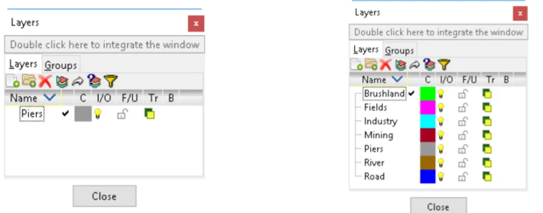
(42) Iber Applications Basic Guide. This model has been created with an old version of Iber. If you are using a more recent version, you will need to transform it to the new problem type (Data>>Problem type>>Iber); select Transform to new problem type and save the model. Note the  has to be visible in Iber problem type. After saving the project, we load the Sat_image.jpg image as a background image (View>>Background Image>>Real size) 5. In this map (Figure 48) we can see the study area. The river crosses from west to east, and there are 4 surfaces which represent the 4 piers of the bridge. Also, on the left bank there are 4 circular culverts (Figure 48, bottom-right).. Figure 48. Study area. View of the background image (left), the geometrical discretization of the piers (top-right) and the culverts (bottom-right). We will prepare two different models in order to consider the piers as a part of the model (Case 1) and as a hole in the mesh (Case 2). But before doing this we will create the geometry of the model, because there are some parts of the models which are common to both cases. An interesting feature of Iber is that it is possible to define specific properties in specific areas (surfaces, lines or points). This can be done easily with the Layers menu (Utilities>>Layers or the button). If we open the Layers window (Figure 49) we can see that there is only one layer called “Piers”. We can create ) layers, and do other things such as change the name (“Name”), change the ( ) and delete 6 (. 5. The georeferenced file has to have the same name as the image file and has to be located in the same folder. 6 Only void layers, without any entities (points, lines and surfaces).. 42.

(43) Iber Applications Basic Guide. colour (“C”), show/not show the layer (“I/O”), block/unblock the layer (“F/U”) and make the layer transparent (“Tr”). For the current example, we will use this tool to create some new layers and to define specific properties (mesh criteria and land uses). The 6 new layers are “Road”, “Fields”, “River”, “Industry”, “Mining” and “Brushland”.. Figure 49. Layers window. On the left the original layers and on the right the specific layer created for this study. We begin by defining the “Road”. Double click on a layer to activate it 7. Using the Create line tool we can now create a polygon that represents the road and the bridge. Bear in mind that we must join this polygon with the existing polygons that represent the piers of the bridge. Then, create the surfaces (Figure 50). Note that the other road (located on the south) is the limit of the model, so it is not necessary to include it.. Figure 50. Representation of the “Road” geometry. On the right side we can observe how the new layer (“Road”) has been joined with the existing one (“Piers”).. 7. Note that the  must be on the layer that we want to use.. 43.

(44) Iber Applications Basic Guide. We continue creating new surfaces corresponding to each layer. The “Mining” area is located downstream of the bridge and the “Industry” area is upstream (it is not necessary to include all its area, see Figure 51, left).. Figure 51. Representation of the “Mining” and the “Industry” geometry (left) and the intersection area of the “River” layer with “Road” and “Piers” layers. The “River” should represent only the actual reach (as shown in the background image). Note that we have to pass over existing layers (“Bridge” and “Piers”). We need to intersect the lines and redraw the geometry to take in account the river discretization (important for the definition of land uses). To do this we use Geometry>>Edit>>Intersection>>Lines and select all the lines of “River” that pass over other layers. Delete the surfaces that have been intersected and redraw the geometry taking in account the layers criteria. Finally, we can create the surfaces that represent the river (Figure 51, right). The “Fields” layer represents some agricultural areas in the study area (on both river banks). To define it, we repeat the same steps shown above. The rest of the model is considered part of the “Brushland” layer. The geometrical discretization is shown in Figure 52. Each layer represents a specific part of the model, and will serve to define both the mesh criteria and the land uses (one Manning coefficient per surface). In this model 8 we are going to define all the properties, and then define the mesh criteria, as a means of considering both Case 1 and 2.. 8. The data provided include the final model, which includes all steps carried out thus far.. 44.

(45) Iber Applications Basic Guide. Figure 52. Final geometrical discretization of the study area.. 5.3.2. Hydrodynamics We introduce the inlet as a Total discharge (subcritical flow) on the “River” line located on the west part of the model. The outlet condition (supercritical/critical flow condition) has been implemented on the east part of the model and must include the whole width of the river and the riverbanks. We will now define the land uses using the geometrical discretization. The Manning coefficient of each layer is defined as follows: “Road” 0.02 s·m-1/3 (corresponding to “infrastructure”); “Mining” 0.075 s·m-1/3 (new creation); “Brushland” 0.05 s·m-1/3 (corresponding to “brushland”); “Fields” 0.028 s·m-1/3 (new creation); “Industry” 0.1 s·m-1/3 (corresponding to “industrial”); “River” 0.035 s·m-1/3 (corresponding to “river”, although the value here must be modified); and “Piers” 0.02 s·m-1/3 (corresponding to “infrastructure”). To create a new Land use you only have to press “New land use” button ( ), introduce the name of the new land use and then define the Manning coefficient. Finally, it is necessary to Update the changes by the button . Note that the land uses of the decks of the bridge must be defined as part of the terrain because the water will flow under the bridge. For this reason, we will consider all the decks of the bridge as land uses of the “river” and the “brushland”. Figure 53 shows the land use discretization.. 45.

(46) Iber Applications Basic Guide. Figure 53. Land uses discretization.. 5.3.3. Culverts Iber has a specific tool for introducing culverts. We understand culverts as hydraulic structures that allow for the transfer of water flow from one point to another. These structures are usually located under roads and rail lines in order to prevent the accumulation of water upstream when a bridge or other structure has been built on a platform higher than the natural topography. This tool has been designed to simulate the working of rectangular and circular culverts (Figure 54). We can introduce one or more culverts using Data>>Hydrodynamics>>Structures>>Culverts. In this new windows we can create, delete and rename culverts. The start and end point of a culvert can be introduced manually or by using the button , selecting any point on the model (the coordinates will be acquired from the topography).. 46.

(47) Iber Applications Basic Guide. Figure 54. Culvert window. Rectangular (right) and circular (left) parameters. In this case, we will define 4 culverts on the left bank of the river, under the road platform. The characteristics of the culverts are as follows: Table 3. Culvert characteristics. Culvert 1 2 3 4. X 477119 477146 477166 477195. Start [m] Y 671757 671718 671673 671629. Z 125.24 126.14 125.31 126.10. X 477181 477200 477227 477252. End [m] Y 671753 671716 671672 671625. Z 125.18 124.54 125.42 125.69. Manning [s·m-1/3] 0.015 0.015 0.015 0.015. Diameter [m] 3 3 3 3. The methodology for implementing culverts is, first, to create the culvert itself using the button . We then need to indicate all the parameters, then Apply. A blue line, with the name of the culvert (“culvertX” by default, where X means the number of the culvert) will be automatically drawn to represent the culvert (Figure 55).. Figure 55. Culvert representation.. 47.

(48) Iber Applications Basic Guide. 5.3.4. Bridges Bridges are one of the most common structures in flood studies. With Iber, a bridge can be introduced as an internal condition in order to modify the shallow water equations accounting for the bridge discharge equations. The bridge condition must be defined on the upstream part of the bridge. We can introduce a bridge using Data>>Hydrodynamics>>Structures>>Bridge. This window (Figure 56) asks for the parameters of the bridge, including the deck elevation (lower and upper part), the bridge opening (if we want to consider obstructions), and the flow coefficients (Cd over the deck; free and submerged pressurized Cd under the deck).. Figure 56. Bridges definition. Parameters of the bridge (left) and green lines considered as a bridge (right). The bridge has a constant elevation (133.5 m) and a height of 2 m (131.5 m on the lower deck). We do not consider obstructions (bridge opening 100 %) and we use the discharge coefficients by default. Once the parameters have been introduced, we Assign on the upstream line that defines the bridge (including the piers part), as shown in Figure 56 (left).. 5.3.5. Mesh Before creating the mesh, we save the model with another name, so that we can simulate two different cases. Case 1 considers the piers as a part of the models, and this implies that we need to introduce the piers as an elevation in the mesh. Case 2 considers the piers as a hole in the mesh, which implies that we should not mesh the area that represents the piers. Nevertheless, some properties of the mesh are common to the two cases. Thus, we are going to assign different mesh sizes. For the “River” layer, this will be 5 m, for the “Roads” layer 3 m, for the “Piers” layer 2 m, and for the rest of the model 10 m. To do this, we use Mesh>>Unstructured>>Assign sizes in the Surfaces menu. 48.

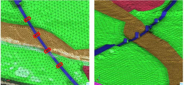
(49) Iber Applications Basic Guide. Case 1. The first step is to generate the mesh and to load the DTM file (DTM.txt) in order to assign the bed elevation to the mesh elements (Iber tools>>Mesh>>Edit>>Set elevation from file). We obtain around 24,000 elements. Second, we need to elevate the piers to the upper part of the bridge deck (133.5 m). To do this, we use Tools>>Mesh>>Edit>>Set elevation constant and assign the elevation to the “Piers” elements (perimeter and interior nodes).. Figure 57. Piers elevation process. Inside the red rectangle are the elements to modify their elevation (left) and the 3D visualization of the topography (right), including the new piers elevation.. Case 2. In the second example, we have to indicate in the model that the “Piers” surfaces must not be meshed. For this we use Mesh>>Mesh criteria>>No mesh in the Surfaces menu and select the appropriate surfaces (Piers”). Remember that we previously defined the bridge condition in the piers, but this condition is an internal condition, and now it becomes a boundary condition, because the piers have not been meshed. Hence we need to unassign the bridge condition. Use the Bridge menu (Data>>Hydrodynamics>>Structures>>Bridge) then repeat the mesh process (generate and elevate the mesh).. 5.3.6. Calculation data In the Problem data window (Time parameters tab) we define the maximum simulation time (7200 s) and the results time interval (120 s). Then Accept the changes.. 5.3.7. Calculation process We have now built the model, and we simply need to calculate it (for both cases). Using Calculate>>Calculate we can begin the simulation. 49.

(50) Iber Applications Basic Guide. 5.4. Results 5.4.1. Hydrodynamic results Here we will compare the two cases as calculated. First, we check whether the maximum water extensions are the same in both cases. Figure 13 shows the maximum inundation, where no significant differences are observed, except in the flow around the piers. These differences are because of the different discretization of the piers, one through the mesh modification (elevation) and the other through a hole in the mesh. In Case 1 there are inclined elements (Figure 57, left) around the piers that cause a different interaction between the piers and the flow. Due to this, a high-water elevation is produced upstream of the piers.. Figure 58. Maximum inundation. Case 1 (left) and Case 2 (right). In this sense, something similar occurs with the velocity field. For example, if we plot the maximum velocity (Figure 59) we can see how in Case 1 we have higher velocities upstream and lower velocities downstream of the piers than in Case 2.. 50.

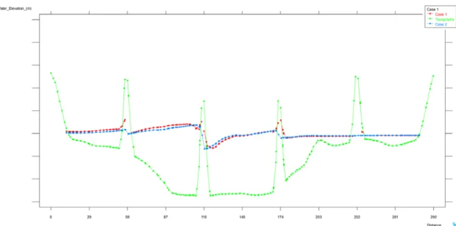
(51) Iber Applications Basic Guide. Figure 59. Maximum velocities. Case 1 (left) and Case 2 (right).. 5.4.2. Bridge results In order to compare the two cases and to see if the water under the bridge reaches the decks, we will now create the maximum water elevation and export it for Case 1. Then, we will plot the same variable in Case 2, in order to compare them. We create a profile using the Graph representation (Window menu). Create a new graph. Select Line Graph of the Maps of Maximums at the end of the simulation (7200 s), and the choose Line Variation of the Water Elevation (m). Apply and then, in the Command line (located at the bottom of the interface), write the coordinates P1 [477228.0,671598.0] and P2 [477396.0,671362.0]. The maximum water elevation has now been plotted (Figure 60).. Figure 60. Maximum water elevation under the bridge. Case 1 (left) and Case 2 (right).. 51.

(52) Iber Applications Basic Guide. For an accurate comparison of the two cases, we will export the graph of Case 2 and import it into the graph set of Case 1. Go to Files>>Export>>Graph and select Line Graph in Road. Step 7200. Iber asks for a name to save it. Then, through Case 1 model we import it (note the graph shown in Figure 60 must be created and open). The data of Case 2’s maximum water elevation is automatically plotted in the same graph set as Case 1. We can now observe the differences between the water elevations (Figure 61). In general, the water level in Case 1 is higher than in Case 2, because in Case 1 the width of the piers is also greater than in Case 2 (in Case 1 we represented the piers as an elevation in the mesh, thus there is a gradual transition between the top elevation of the pier and the topography) 9.. Figure 61. Comparison of the maximum water elevation under the bridge in Case 1 and in Case 2.. 5.4.3. Culver results Iber allows the user to see which part of the flow is transferred by the culverts. Since version 2.4.3 of Iber, these results are saved in a file called “Culverts.grf” (previously they were saved in “Culverts.rep”, and this file can be opened in Notepad or any other text-based application). We can observe (Figure 62, top), in both cases, how the culverts transfer a notable amount of water from upstream to downstream of the bridge (around 125 m3/s). The closest culverts to the river (Culverts 3 and 4) transfer less water than Culverts 1 and 2. This is because there is a depression on the left bank of the river due to the presence of an old meander. This meander affects the culverts and also the flow field. We can see how the water flows from downstream to upstream on the left bank during the first time steps of the simulation.. 9. Note that the name and colours of the lines have been changed using the Options tab.. 52.

(53) Iber Applications Basic Guide. Figure 62. Evolution of the flow through the culverts in Case 1 (top-left) and Case 2 (top right). Topography elevation map (bottom).. 5.5. Conclusions In this example we have introduced some methodologies and modelling techniques to improve flood studies. The implementation of bridges and culverts allows us to reproduce more accurately the reality of a given situation (Bladé et al., 2014a). Bridges in Iber are treated as an internal condition. This condition considers two dimensions of the space, and means that if the flow passes obliquely to the condition, Iber will respect this flow condition and will interact and modify the hydrodynamics to take in account the 2D phenomenon (e.g. the water elevation is greater than the deck elevation). Two different ways for representing the piers of the bridge (Case 1 as a part of the model, and Case 2 as a hole in the mesh) have been shown. Both cases are valid in these conditions (water elevation is less than the deck elevation of the bridge), but only Case 1 is valid when the water elevation reaches and exceeds the bridge deck. 53.

(54) Iber Applications Basic Guide. Culverts is an interesting means of allowing the transfer of flow between two points. Commonly used on road and train lines to allow small reaches to continue or for avoiding flooding upstream, we need to be able to see how these work in both case studies. The amount of flow transferred depends on the water level and the characteristics of the culvert (size, slope and roughness). This chapter has also served to introduce the layers management tool and how to use it for defining certain properties. In the postprocess, we have seen how to export and import results, and to compare them in the same graph set.. 5.6. References Bladé, E., Cea, L., Corestein, G., Escolano, E., Puertas, J., Vázquez-Cendón, E., Dolz, J., Coll, A. (2014a). Iber: herramienta de simulación numérica del flujo en ríos. Revista Internacional de Métodos Numéricos para Cálculo y Diseño en Ingeniería, Volume 30, Issue 1, 2014, Pages 1-10, ISSN 02131315, DOI: 10.1016/j.rimni.2012.07.004 Bladé, E., Cea, L., Corestein, G. (2014b). Modelización numérica de inundaciones fluviales. Ing. del agua 18, 68. DOI: 10.4995/ia.2014.3144 Cea L, Puertas J. Flood modelling with the software Iber. In: II International Congress on Water: Floods and Droughts. Ourense. 27-28 Octubre 2016; 2016. González-Aguirre JC, Vázquez-Cendón ME, Alavez-Ramírez J. Simulación numérica de inundaciones en Villahermosa México usando el código IBER. Ing del Agua. 2016;20(4):201. DOI: 10.4995/ia.2016.5231. 54.

(55) Iber Applications Basic Guide. 6. Practical Example 4: Dam break 6.1. Objectives This example introduces the user to dam break analysis using Iber. The Breach tool will be explained, which allows us to define the shape and other properties of the breach formation process. We will analyse the water depth evolution in a reservoir and downstream of a dam, and also the maximum water elevation in the village located downstream. The way to represent the breach formation and its effects on the modelling process will be shown, as well as how to create hydrographs. This chapter will serve as a brief review of mesh properties and other criteria dealt with in previous chapters, and also to introduce Iber’s tools for creating graphs in the postprocess.. 6.2. Description of the case study and input data This example involves the analysis of a dam break and the effects provoked by flood inundation downstream. The Bayco u Ortigosa reservoir was built to avoid floods on the Ortigosa River. The reservoir is located in the southeast of Spain, occupies 111.54 ha and has 6.2 hm3 of storage capacity. The dam is 648 m long and 43 m high.. Figure 63. Representation of the dam. The presence of a village (Ontur, at south) is the reason for a dam break analysis. The data provided consist of a Digital Terrain Model, which has a 5x5 m cell size resolution (DTM.txt) and includes the dam (Figure 63), and a background images (maps of the study area, Map.jpg and Map.jgw). The geometry of the model will be set up after a topographical analysis of the study area, and will be refined after considering the model results.. 55.

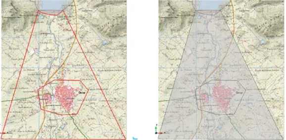
(56) Iber Applications Basic Guide. 6.3. Model set-up 6.3.1. Geometry After saving the project, we will load the map as a background image Map.jpg (View>>Background Image>>Real size). This image is a georeferenced map located in the real UTM coordinates 10. Though this map (Figure 64) we can see the reservoir located to the north (in light blue), Ontur village to the south (in pink), plus the contour topography lines (in brown). The reservoir limit and the contour lines will serve to define the geometry of the model.. Figure 64. Study area. View of the background image (top-left), the geometrical discretization of the reservoir (top-right), the dam (bottom-left) and the rest of the model (bottom-right).. 10. The georeferenced file must have the same name as the image file, and has to be located in the same folder.. 56.

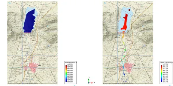
(57) Iber Applications Basic Guide. Using the geometry tools, we will create three surfaces (reservoir, dam and the rest of the model). First, we define the reservoir. Zoon in ( ) to the reservoir and draw the perimeter with a generous offset (Figure 64, top-right). For the dam, we will define another polygon, bearing in mind that the dam has a variable width downstream (Figure 64, bottom-left). Finally, for the rest of the model we extend this area from the corners of the dam to the southernmost part of the model 11 (Figure 64, bottom right). It might be useful to define a more accurate mesh in the village and its neighbourhood. For this reason, we will create another surface on the village. We delete the surface located downstream of the dam (Figure 64, bottom-right) and create another polygon with the village inside it. We create the surfaces by selecting, first, the external and the internal lines, in order to consider the village area as a hole in the external surface (Figure 65, left). Then we create the village surface (Figure 65, right).. Figure 65. Village surface definition. View of the selected lines of the rest of the model polygon (left) and the result of this surface creation process (right).. 6.3.2. Hydrodynamics We define as the outlet boundary condition the southernmost line of the model. A priori, we do not know what the flow condition on this boundary is. Nevertheless, our study area is limited to the village, thus we can assign a supercritical flow, because the outlet is far away from the study area. This model does not have a defined inlet boundary condition 12. The initial condition will be assigned only on the reservoir surface (Figure 64, top-right). The value of this condition is 687 metres (Elevation). We use “river” as a land use (0.025 s·m-1/3) for the whole model except for the Ontur village (residential, 0.15 s·m-1/3).. 11. The DTM extension is no longer than the image. Do not overdo it. Iber can work without boundary conditions (e.g. the inundation process of a channel considering only an initial water volume). 12. 57.

(58) Iber Applications Basic Guide. 6.3.3. Mesh The geometrical definition will serve to define different element sizes. We have two zones where the hydrodynamics must be more accurate than for others. The dam and the village are important for the study because the breach will be formed in this area and we need more detailed results in the village. We will now define the following element size (Mesh>>Unstructured>>Assign sizes on surfaces): • • • •. Reservoir: 200 m Dam: 5 m Village: 15 m Rest of the model: 50 m. We can check the mesh size assigned using Mesh>>Draw>>Sizes>>Surfaces (Figure 66 left). Once the mesh criteria have been checked, we generate the mesh. The value requested during Mesh generation is 250 m. The model will have around 35000 elements (Figure 66).. Figure 66. Mesh criteria. Mesh size of each surface (left) and mesh model in each zone (right). Once the mesh has been generated, we load the DTM file (DTM.txt) to assign the elevation on the mesh elements (Iber tools>>Mesh>>Edit>>Set elevation from file).. 6.3.4. Breach Iber has a specific tool for introducing the breach parameters. It will read these and will make a mesh deformation in order to reproduce the evolution of the breach, allowing the exit of the water over the breach. 58.