Differences in wage determination in the Eurozone: A challenge to the resilience of the common currency

Texto completo

(1)Differences in wage determination in the Eurozone. by Mariam Camarero Gaetano D’Adamo and Cecilio Tamarit September 2018. Working Papers in Applied Economics Economics WPAE-2018-11. Departamento de Estructura Económica (Economía Aplicada II), Facultad de Economía, Universitat de València Avda dels Tarongers, s/n, 46022 – Valencia, Spain Phone +34 96 382 83 49 / Fax +34 96 382 83 54 http://www.estructuraeconomica.es ISSN 2172-3036 e-mail: investigacion.estructura@uv.es.

(2) Differences in wage determination in the Eurozone. Mariam Camareroa; Gaetano D’Adamob ; Cecilio Tamaritc. a. INTECO Joint Research Unit, Department of Economics, University Jaume I. Campus de Riu Sec E-12071 Castellón de la Plana, Spain. b. Directorate-General for Economic and Financial Affairs, European Commission Rue de la Loi 170, 1000 Brussels, Belgium. c. INTECO Joint Research Unit, Department of Applied Economics II, University of Valencia. Av. dels Tarongers s/n 46022 Valencia, Spain.. Abstract This paper estimates a simple equilibrium wage equation for a subset of Eurozone countries over the period 1995-2015 using panel cointegration methods that account for cross-country heterogeneity and allow for structural breaks. Results show that the equilibrium wage has been affected by a structural change contemporaneous to the international financial crisis. Moreover, it has different determinants across euro area countries, among which two relatively distinct groups can be identified. In particular, the wage equation in Germany, Austria, Belgium, the Netherlands and Finland is more homogeneous and seem to respond more to macroeconomic conditions than in the group composed of Italy, Spain, Portugal, France and Ireland. This result is highly policy relevant in the context of a single monetary policy, as it may explain the diverging behavior of wages across the Eurozone and also be a potential source of asymmetric shocks and/or asymmetric response to a common shock.. JEL Classification: E24; C23 Keywords: panel cointegration, wage setting, labor market, productivity, real exchange rate.. *. Corresponding author. E-mail address: gaetano.d'adamo@ec.europa.eu. Most of the research was performed when Gaetano D'Adamo was Assistant Professor at the University of Valencia. The views expressed here are those of the authors and do not necessarily reflect those of the European Commission. All remaining errors are the sole responsibility of the authors. The authors gratefully acknowledge financial support from MINEICO and Feder project ECO2017-83255-C3-3-P.. 1.

(3) 1. Introduction The objective of this paper is to answer the following questions: are euro area countries similar in terms of wage determination? If that is not the case, can we identify alternative "models" of wage determination across groups of euro area countries? To this end, we estimate a very simple long-run wage equation for a subset of the euro area using panel cointegration techniques that allow for country heterogeneity and the existence of (unknown) structural breaks. The prevalence of different labour market "models" in the EU has been already highlighted, for example, by Boeri (2002) following Ferrera (1998). According to Boeri, four models of social policy prevailed in the EU-15 at the end of the 20th century: Nordic, Continental, Anglo-Saxon and Mediterranean.1 Sapir (2006), on the same page, evaluated the performance of these four models according to the criterion of labour market participation in terms of efficiency (i.e. relatively high employment rates) and equity (i.e. keeping the risk of poverty relatively low). In his analysis, Nordic countries scored best on both criteria; the continental model provided equity at the price of somewhat low efficiency while the opposite held for Anglo-Saxon countries. Finally, Mediterranean countries scored badly on both dimensions. Almost two decades have passed since Ferrera (1998) had identified these four models and most countries in the EU-15 have adopted the euro and undergone. 1. The Nordic model included Denmark, Sweden, Finland and the Netherlands (which were considered. a hybrid with the Continental model); the Continental model included Belgium, France, Germany and Luxembourg; the Anglo-Saxon included UK and Ireland and the Mediterranean model included Italy, Spain, Portugal and Greece.. 2.

(4) substantial labour market reforms in the meantime, not to mention the shock to labour markets represented by the global economic and financial crisis. These reforms have contributed, to some extent, to a convergence in the social/institutional models of EMU countries It is therefore an important empirical and policy question to ask whether substantial differences in labour market models and, in particular, wage determination in the euro area still persist. At the start of the Economic and Monetary Union (EMU), it was somewhat expected that the adoption of a single currency would give strong incentives to carry out structural reforms that would compensate for the loss of monetary policy as a stabilization tool, and therefore "structural convergence" would occur as a by-product of nominal and real convergence. However, the facts have proved that this expectation was only partly true, and a large effort in terms of structural reforms (both in product and labour market) has been instead made, at least in the countries most heavily hit by the crisis, as a result of the global economic and financial crisis of 2008-2009 and the subsequent sovereign debt crisis. Understanding wage determination in the euro area is a matter of primary policy relevance, as demonstrated by the emphasis that the OECD, the IMF, the European Commission and the ECB, among others, have put on labour market reforms and wage flexibility in recent years, if anything because of the relevance of labour market dynamics for the smooth functioning of the monetary union.2 The importance of the topic for the euro area is, in fact, threefold. First and foremost, wage developments have important second-round effects on prices and, therefore,. 2. See, for instance, OECD (2004), IMF (2014), EC (2016) and ECB (2012).. 3.

(5) potentially on (price) competitiveness.3 Specifically for euro area countries, in the absence of the nominal exchange rate as an adjustment tool, excessive inflation (relative to the rest of the Monetary Union) has to be corrected, sooner or later, via internal devaluation. This has, indeed, been the experience of a number of EMU countries that have undergone significant adjustment in the wake of the euro area sovereign debt crisis. Secondly, heterogeneity in the functioning of labour markets in the euro area is a potential source of asymmetric shocks and/or asymmetric response to a common shock and is thus relevant in the context of a single monetary policy. Such heterogeneity may be due to institutional factors, like the degree of employment protection, the level of bargaining coordination or the type of wage leadership across sectors, since leadership of a non-traded sector in some countries may be conducive to wage non-moderation, other things equal.4 Indeed, Jaumotte and Morsy (2012) have recently shown that high employment protection and intermediate coordination in collective bargaining have contributed significantly to the high and persistent inflation differentials of several EMU countries in the run-up to the crisis. Thirdly, labour and. 3. For example, Estrada et al. (2013) highlight persistent inflation differentials and, as a result, large. cumulative changes in relative prices, within the EMU, at least until 2007. Such dynamics seem to reflect, to a large extent, the underlying patterns of unit labour costs and wages. However, the authors also challenge the view that these divergences caused the observed current account imbalances in the run-up to the crisis. 4. In a recent work, Camarero, D’Adamo and Tamarit (2014) studied in a country-by-country basis the. wage leadership theory in the context of the euro area members over the period 1995-2010. Results point to the public sector being the leader in Germany, Belgium and Greece, whereas construction drives wages in Ireland and Spain. The results also show that the response to positive versus negative shocks is asymmetric in the Mediterranean countries, Ireland and the Netherlands.. 4.

(6) product market which are more responsive to shocks allow for smooth resource reallocation and therefore increase the resilience of the economy. In a recent paper, Camarero et al. (2016), estimated the wage equation for the euro area using panel cointegration techniques and accounting for labour market institutions, finding that more flexible labour market institutions are compatible with wage moderation, and that, after the Eastern enlargement, the importance of productivity and real exchange rate dynamics in explaining wage developments increased with respect to institutional factors and unemployment. Furthermore, previous research (Arpaia and Pichelmann 2007) has, in fact, shown that labour cost developments in the euro area have not always reflected warranted adjustments, but rather different degrees of wage flexibility across countries. One may therefore ask whether we can indeed assume that a common wage equation for the whole EMU exists or clusters of labour market models can be identified in the Monetary Union. Against this background, in the present paper we estimate a simple model of the wage equation for a subset of Eurozone countries, paying special attention to the common patterns and differences among EMU member states, using panel techniques that allow for cross-country heterogeneity and structural breaks and quarterly data for the period 1995-2015. In particular, we estimate longrun relationships, allow for structural changes in the deterministic components and / or in the cointegration parameters, and test for homogeneity in the panel. The application of the method of Pesaran et al. (1999), that is, the Pool Mean Group Estimator (or PMGE), to the data allows us to test statistically the homogeneity of wage equation. In this way, we identify two relatively distinct groups of countries: on one side Germany, Austria, Belgium, the Netherlands, Luxembourg and Finland, with. 5.

(7) a more dynamic wage determination, and on the other side France, Italy, Spain, Portugal and Ireland with a more heterogeneous wage determination model. The paper is organized as follows: after this introduction, the second section defines the wage equation and section 3 presents the dataset and the econometric methodology. Section 4 reports the results of the analysis assuming a common wage equation for the EMU while section 5 introduces the results allowing for crosscountry heterogeneity. Section 6 concludes.. 2. The Wage Equation The wage equation is a key element of any comprehensive model of the macroeconomy. The relationship between wages and unemployment à la Phillips (1958), and more generally the equilibrium equation for the real wage, has been extensively estimated in the literature since Blanchflower and Oswald (1994). 5 We can interpret the observed real wage as the result of the bargaining process between employees’ unions and employers. On the supply-side, unions push for wage increases above productivity, but their bargaining power depends on the unemployment rate since wage demands tend to be more moderate when unemployment is high. Therefore, we can write 𝑤𝑎𝑔𝑒𝑡𝑠 = 𝑓(𝑝𝑟𝑜𝑑𝑡 , 𝑢𝑛𝑒𝑚𝑝𝑡 ); 𝑓 ′ 𝑝𝑟𝑜𝑑 > 0, 𝑓 ′ 𝑢𝑛𝑒𝑚𝑝 < 0. (1). where 𝑤𝑎𝑔𝑒𝑡 is the (log) real wage; 𝑝𝑟𝑜𝑑𝑡 is (log) labor productivity and 𝑢𝑛𝑒𝑚𝑝𝑡 is the unemployment rate. The existence of a positive relationship between the level of. 5. See, for example, Nunziata (2005), Marcellino and Mizon (2000), Alesina and Perotti (1997), Baltagi. et al. (2000).. 6.

(8) the real wage and productivity, on one hand, and a negative relationship between the unemployment rate and the real wage is, indeed, what is implied by Blanchflower and Oswald’s (1994) “wage curve” as well as matching models (see Blanchard and Katz, 1997). On the labor demand side, employers tend to constrain the real wage, maximizing their mark-up on unit labor cost (ULC), where the latter are defined as 𝑤𝑎𝑔𝑒𝑡 − 𝑝𝑟𝑜𝑑𝑡.6 The mark-up that employers will be able to extract from the real wage will in turn, be constrained by competitive pressures coming from foreign producers, which can be proxied by the real exchange rate. In principle, the real exchange rate can affect labor costs in different ways. First, a fall in the real exchange rate (i.e. depreciation) increases the demand for domestic goods, thus raising labor demand and the real wage (Campa and Goldberg 2001). We will call this channel the labor demand channel. Second, when the real exchange rate decreases, increasing the cost of imported final goods, this induces workers to attempt to maintain their real net incomes, increasing wage pressure (wage bargaining pressure channel; Nunziata, 2005). Third, depreciation increases the price of imported intermediate goods and thus production costs; to the extent that those goods are complement to labor, it will foster a reduction in labor demand and in the real wage (imported intermediate goods channel; Robertson, 2003). Fourth, depreciation of the real exchange rate implies that imported goods are more expensive, which makes the consumer price index increase and real wage decline (imported inflation channel). If we define the real effective exchange rate as units of (trade-weighted) foreign goods per unit of domestic goods, the first and second channel would imply a negative relationship between 𝑤𝑎𝑔𝑒𝑡 and. 6. Employers’ mark-up on ULCs may be expressed as the opposite of ULC.. 7.

(9) the real exchange rate, while the third and fourth would imply a positive relationship. On the demand side, we can therefore write 𝑤𝑎𝑔𝑒𝑡𝑑 = 𝑔(𝑝𝑟𝑜𝑑𝑡 , 𝑟𝑒𝑒𝑟𝑡 ). (2). ′ where 𝑔′𝑝𝑟𝑜𝑑 > 0; 𝑟𝑒𝑒𝑟𝑡 is the real exchange rate and 𝑔𝑟𝑒𝑒𝑟 ≷ 0 depending on which. of the channels described above prevails. Therefore, by combining the labor supply and the demand side and in analogy with existing work (Nickell, 1998; Bell et al. 2002; Nunziata 2005), the equilibrium wage equation can be written as a reduced-form specification suitable for estimation, incorporating both demand- and supply-side factors: 𝑤𝑎𝑔𝑒𝑡 = 𝛽0 + 𝛽1 𝑝𝑟𝑜𝑑𝑡 + 𝛽2 𝑢𝑛𝑒𝑚𝑝𝑡 + 𝛽3 𝑟𝑒𝑒𝑟𝑡 + 𝜀𝑡. (3). where we expect, a priori, 𝛽1 > 0, 𝛽2 < 0 and 𝛽3 ≷ 0. The problem with equation (3) is that coefficients cannot be interpreted structurally due to a simultaneity problem: the level of the wage affects prices and therefore the real exchange rate. On the other hand, our wage equation may be affected by the potential endogeneity, in particular, of the real exchange rate. However, our empirical approach overcomes these problems. On the one hand, as long as the variables in (3) are non-stationary I(1) and co-integrated, equation (3) can be interpreted as a long-run equilibrium relationship and we can estimate it in errorcorrection form: ∆𝑤𝑎𝑔𝑒𝑡 = 𝛾0 + 𝜸1 ∆𝒙𝑡−1 + 𝛼(𝑤𝑎𝑔𝑒𝑡−1 − 𝛽0 − 𝛽1 𝑝𝑟𝑜𝑑𝑡−1 − 𝛽2 𝑢𝑛𝑒𝑚𝑝𝑡−1 − 𝛽3 𝑟𝑒𝑒𝑟𝑡−1 ) + 𝜗𝑡. (4). where 𝒙 is the vector including our four variables of interest from equation (3) lagged and the term within parentheses on the right-hand side is the error term in (3) in t-1.. 8.

(10) The coefficient 𝛼 is the error-correction coefficient; thus, as long as 𝛼 < 0 and significant, whenever a disequilibrium in (3) occurs due to a shock to 𝑝𝑟𝑜𝑑, 𝑢𝑛𝑒𝑚𝑝 or 𝑟𝑒𝑒𝑟, wages will adjust to bring us back to equilibrium. In other words, if 𝛼 < 0 the equation is identified from an economic point of view, since the dependent variable in (3) is actually responding to disequilibria. Since −1 < 𝛼 < 0, the closer α is to -1, the less sticky the wages. On the other hand, to address the issue of endogeneity, as a robustness check we will estimate equation (4) using the nominal effective exchange rate in place of 𝑟𝑒𝑒𝑟. We will come back to this point in Section 4.. 3. Data and Empirical Methodology In order to estimate Equation (4), we used quarterly data from 1995Q1 until 2015Q4 on the group of countries commonly known as EMU-11: Austria, Belgium, Finland, France, Germany, Ireland, Italy, Luxembourg, Netherlands, Portugal and Spain. In order to work with a balanced panel but with sufficiently long series, on the one hand the more recent EMU Member States had to be excluded and, on the other hand, the time span has been restricted to this period due to data limitations for some of the countries involved. For the same reason, the remaining current member states of the EMU were excluded. Data for all 11 countries in the sample come from Eurostat and variables are seasonally and working day adjusted. Wages have been calculated as real compensation per employee and, consistently, productivity is gross value added. 9.

(11) per employee.7 Finally, nominal wages have been transformed into real deflating with the Harmonized CPI. A preliminary analysis showed that the four variables of interest (𝑤𝑎𝑔𝑒𝑡 , 𝑝𝑟𝑜𝑑𝑡 , 𝑢𝑛𝑒𝑚𝑝𝑡 and 𝑟𝑒𝑒𝑟𝑡 ) are all I(1) in levels.8 Since all variables are I(1), we proceeded with the cointegration analysis. In order to test for cointegration, we used the panel statistics proposed by Banerjee and Carrion-i-Silvestre (2013). The main advantage of this approach is that it allows for a break in the cointegration relation, where the date of the break is unknown a priori, and therefore the specification of the long-run model can be chosen from a total of six possible specifications: from a standard cointegration relation with an intercept up to specifications allowing for structural changes both in the deterministic and the cointegrating vector. Table 1. Banerjee and Carrion (2013) panel cointegration tests f(prodit, reerit, unempit). Model. 𝑍𝑗∗. AIC. BIC. 1 2 3 4 5 6. -2.94 -4.52 -4.82 -4.35 -3.11 -4.22. -8.60 -8.98 -9.26 -7.92 -8.85 -9.29. -8.31 -8.63 -8.86 -7.46 -8.33 -8.71. Note: Critical values of the Zj* are -2.824, -2.113 and -1.759 at 1percent, 5percent and 10percent significance levels, respectively, for the model with constant, whereas -2.924, -2.240 and -1.835 are their equivalents in the model with trend.. 7. One may argue that it may be preferable to use hours worked rather than the number of employees as. denominator to calculate the wage and productivity, in order to exclude effects coming from changes in the share of part-time workers. However, in our case this would have implied shorter time series for some of the countries, which would be problematic given that the time span considered is already quite short. 8. Results of the unit root tests are available from the authors upon request.. 10.

(12) As shown in Table 1, using the Banerjee and Carrion (2013) test, we applied the statistic based on the accumulated idiosyncratic components, Zj*. We present the test for all possible specifications; in all cases the null hypothesis of non-cointegration is rejected. Moreover, according to the information criteria 9, the appropriate model could be either Model 3 (constant and trend restricted in the cointegration relation, and a break in both) or Model 6 (the break affects the level, the trend and the cointegrating vector, i.e. there is a “regime break”). The break is found to be in 2004Q3 in Model 3 and 2009Q3 using Model 6. The break in Model 3 is the same as Camarero et al. (2016), where the sample period was 1995-2011. In that paper, this break was interpreted as the impact on wage determination of the EU enlargement, which increased competitive pressures on exporters as well as within-Europe migration flows. When allowing for a regime break, in Model 6, the break date we find approximately coincides with the global economic and financial crisis. This is not a surprise, given the large shock implied by the crisis and, at the same time, the fact that some sample countries adopted a number of structural reforms between 2009 and 2015 which increased the flexibility of the labor market. The Banerjee and Carrion (2013) test thus suggests that the preferred models include a trend in the cointegration relation. While including a linear trend in the equilibrium relationship may be criticized since it is difficult to interpret economically, on the other hand it allows us to define the cointegration as one. 9. Using AIC we would have chosen Model 6, whereas according to BIC the best specification would be. Model 3. Therefore, we present the results for both models. Moreover, the comparison between the two models is also interesting, as Model 6 allows for a structural change in the cointegrating relationship.. 11.

(13) between the real wage and trend-adjusted productivity (plus other variables), where the trend proxies technological progress 10. Starting with these two alternative specifications and in order to dig deeper into the long-run determinants of the real wage in the EMU, we estimate the long-run regressions – accounting for the structural breaks found above – using the heterogeneous pooled mean group estimator by Pesaran et al. (1999), henceforth PMGE. Following a general-to-specific approach, we will then test whether it can be assumed that the long-run parameters for the 11 countries in the group, or at least some of them, are equal across the panel. Pesaran and Smith (1995) observe that while it is implausible that the dynamic specification is common to all units, it is at least conceivable that the long-run parameters of the model may be common. The cross-sectional dimension can then be exploited to gain more precise estimates of these average long-run parameters. They then propose estimation by either averaging the individual unit estimates (the Mean Group method: MG), or, in their later paper with Shin (Pesaran et al., 1999) by pooling the long-run parameters with the PMG method. The PMG estimator therefore involves both pooling and averaging: the intercepts, short-run coefficients and error variances differ freely across groups, but the long-run coefficients are constrained to be the same. An interesting feature of this methodology is that some of the long-run parameters can be also unconstrained so that they may be different for each group. This possibility, which can be tested using LR-type tests, is especially appropriate for 10. Moreover, including a linear term is a standard procedure in cointegration analysis when the. variables included seem to exhibit a deterministic trend, other than a stochastic trend, and the slope of such trend is different across variables. In this case, excluding the trend from the cointegration relation may leave us with residual non-stationarity. See also Juselius (2006).. 12.

(14) this case. Moreover, an additional advantage of this approach is its usefulness for general-to-specific analysis in a panel cointegration context. The analysis is carried out in several stages. The first consists of the specification of the statistical model11, where the lag order of the Autoregressive Distributed Lag (ARDL) model is selected using information criteria (Akaike's AIC and Schwarz’s). In the second stage, the relevant variables are chosen and alternative model specifications are compared, also using information criteria. Next, the hypotheses about the homogeneity of the long-run parameters are tested. Fourth, for additional specification tests for the models, the individual equation statistics should be analyzed. Finally, the null hypothesis of non-cointegration can be tested using the error-correction t-statistics for both the system and the country-equations.. 4. A Eurozone-wide wage equation Taking into account the previous findings concerning the structural break and the deterministic specifications, we have filtered the variables from the deterministic components before proceeding to the application of the PMGE procedure. The added value of the approach we perform here is that, when estimating the wage equation in error correction form, it allows us to test for the restriction of equality of (some) longrun coefficients, while leaving other coefficients free to change across countries. We start by estimating a single wage equation for the EMU-11 and testing for coefficient homogeneity within the full group. Afterwards, in Section 5, we will investigate how. 11. For estimation, we require a dynamic model with a long-run solution. As we do not have any. specific theory of the short-run dynamics, we specify a general ARDL in the logs of the variables entering the equation.. 13.

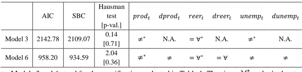
(15) different groups or clusters of countries can be identified based on the estimated wage equations.12 As shown in Table 2, we could not impose cross-country coefficient homogeneity for all variables in the long-run relationship. The restricted models that could not be rejected are reported in the Table. Table 2. Coefficient homogeneity restrictions – EMU-11 AIC. SBC. Model 3. 2142.78. 2109.07. Model 6. 958.20. 934.59. Hausman test [p-val.] 0.14 [0.71] 2.04 [0.36]. 𝑝𝑟𝑜𝑑𝑡. 𝑑𝑝𝑟𝑜𝑑𝑡. 𝑟𝑒𝑒𝑟𝑡. 𝑑𝑟𝑒𝑒𝑟𝑡. 𝑢𝑛𝑒𝑚𝑝𝑡. 𝑑𝑢𝑛𝑒𝑚𝑝𝑡. ≠∗. N.A.. = ∀∗. N.A.. ≠∗. N.A.. ≠∗. ≠. = ∀∗. =∀. ≠. ≠. Note. Models 3 and 6 stand for the specifications selected in Table 1. The signs ∀∗ and ≠ denote homogeneity and heterogeneity of the estimated parameters, respectively. An asterisk means that the variable is significant. N.A. = not applicable.. First of all, the results are slightly different depending on whether we choose Banerjee and Carrion-i-Silvestre's (2013) Model 3 (a change in the deterministic components) or Model 6 (a change in both the long-run relation and the deterministic components). In both cases, only the null hypothesis of homogeneous parameters for the real exchange rate across the participating countries cannot be rejected. Instead, the coefficients of productivity and the unemployment rate differ across countries. This is no surprise, given the large institutional labor market differences that are. 12. Note that this approach is different from the one we followed in Camarero et al. (2016): while in that. model institutional variables were included in the long-run relations, and therefore cross-country differences in the wage equation were assumed to be captured by the different labor market institutions, in the present paper we imply that different structures and institutions of the labor market result in long-run heterogeneity.. 14.

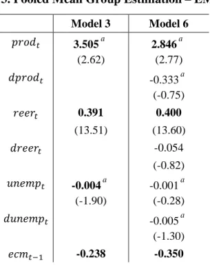
(16) present across the sample.13 Furthermore, the breaks in the coefficients in Model 6 are not significant. Detailed (group) coefficient estimates are reported in Table 3.14 All coefficients have the expected signs; a real effective exchange rate appreciation triggers a rise in the real wage. Moreover, there is significant error correction, the coefficient on 𝑒𝑐𝑚𝑡−1 implying that it takes between 3 and 4 quarters, other things equal, for wages to adjust to a disequilibrium. However, as mentioned above, some parameters could not be constrained to being equal, and therefore the mean group estimates of productivity and unemployment, in particular, imply significant cross-country differences. This may suggest that further insight could be gained by grouping countries in smaller clusters for which homogeneity restrictions may hold. This is the aim of the following section. Table 3. Pooled Mean Group Estimation – EMU-11 Model 3 𝑝𝑟𝑜𝑑𝑡. a. 3.505 (2.62). 𝑑𝑝𝑟𝑜𝑑𝑡 𝑟𝑒𝑒𝑟𝑡. Model 6 a. 2.846 (2.77) a. -0.333 (-0.75) 0.391. 0.400. (13.51). (13.60). 𝑑𝑟𝑒𝑒𝑟𝑡. -0.054 (-0.82). 𝑢𝑛𝑒𝑚𝑝𝑡. a. -0.004 (-1.90). 𝑑𝑢𝑛𝑒𝑚𝑝𝑡 𝑒𝑐𝑚𝑡−1. 13. a. -0.001 (-0.28) a. -0.005 (-1.30) -0.238. -0.350. For example, unions’ bargaining power, the existence of a minimum wage or the degree of. unionization. See Briscoux et al. (2014) for a very detailed discussion and comparison of the minimum wages in the EU and Chevreux and Darmaillacq (2014) for the level of unionization. 14. Individual country estimates for both models are reported in Appendix 1.. 15.

(17) (-8.86). (-9.87) a. Note: Dependent variable: waget. t-Students in parentheses. indicates that the corresponding variable was not subject to the restriction of equal long-run parameters for all the members of the group. Thus, its estimate is the Mean Group Estimate, instead of the PMGE.. 5. Two different models of wage determination in the EMU-11 Since the previous analysis highlighted that a single wage equation for the EMU could not be found, given that only the coefficient of the real exchange rate was found to be homogeneous, we proceeded looking for subgroups of countries for which a more homogeneous wage equation could be found. To this end, we have tested for alternative subgroups for which homogeneity restrictions could be imposed. The results indicate that two groups with rather different wage formation models can be identified among the EMU-11 countries. The first group is composed of Germany, Austria, Belgium, Luxembourg and the Netherlands, while the second consists of Spain, Italy, France and Ireland. The composition of these groups shows a quite close correspondence with the groups based on different labour market/social models identified in Boeri (2002) and Sapir (2006), with the exception of France. 15 In particular, our first group corresponds to the "Continental" and "Nordic" models whilst the second broadly corresponds to "Mediterranean", plus Ireland and France. For reasons of convenience, we will call the two groups "Core" and "Periphery".16. 15. While the fact that France ends up in a different group compared to Boeri (2002) might seem. surprising, within the present analysis, whenever France was included in the group of the Continental and Nordic model, we could not find a long-run model where restrictions of within-group coefficient equality were not rejected. Moreover, indeed within the present framework and from the point of view of labor market functioning, France shares a number of features with Mediterranean countries. 16. France might be included among "periphery" countries also according to other criteria. For example,. Buti and Turrini (2015) grouped Centre and Periphery euro area countries according to their external. 16.

(18) Table 4. Summary Statistics: two labour market models. Compensation per Employee Unemployment rate Labor Productivity Real Effective Exchange Rate Union Density 17 Employment Protection Coordination in Wage Bargaining. AT, BE, DE, FI, NL, LU Sample mean 8.67 6.72 15.79 101.99 40.57 2.23 3.67. ES, FR, IE,GR, PT Sample mean 6.22 10.71 12.57 95.81 23.49 2.61 3.41. Source: Eurostat, ICTWSS Database, OECD and authors’ calculations. The reference sample is 19952016 for Compensation per Employee, unemployment rate, labor productivity, real effective exchange rate; 1995-2014 for Union Density and 1995-2013 for EPL and Wage Coordination, due to data availability.. As shown in Table 4, when looking at the model variables and several labour market institutions, from a descriptive point of view we can say that the Core’s labor market is more “dynamic” while the Periphery’s is more “sluggish”: in fact, the former shows, on average, higher compensation per employee and labor productivity, lower unemployment rate and is more decentralized and flexible, while it is more unionized18. By dividing the sample in two groups and allowing some of the coefficients to still change across countries, therefore, we are implicitly accounting for institutional and other differences across our sample units. Tables 5 and 6 report. position and included France in the periphery. With few exceptions, countries in the centre recorded a surplus over the 1999-2009 period, while periphery countries recorded a deficit. 17. Since France is an outlier in terms of UD, with an average membership rate over the sample of 7.9%,. we also calculated this mean excluding France. Still, the average UD in the "periphery" is 27.4%, well below that of the "core". 18. In the case of France, Chevreux and Darmaillacq (2014) point out that, while France has one of the. lowest degrees of union membership in the OECD, it also has one of the highest rates of collective bargaining coverage (over 90%). As in other peripheral EU countries, low union density does not diminish the degree of representation of the workers, as the pacts reached by the unions and the employers are generally extended to the majority of the workers.. 17.

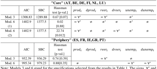
(19) the results of Pesaran’s PMGE. We will first discuss the results of the Hausman tests on the homogeneity restrictions (Table 5) and then the point estimates obtained using Carrion-i-Silvestre’s (2013) Model 3 (break in constant and trend) and Model 6 (regime break). Table 5. Coefficient homogeneity restrictions – Country Groups "Core" (AT, BE, DE, FI, NL, LU). Mod. 3 Mod. 6 (1) Mod. 6 (2). AIC. SBC. 1308.83 1402.9. 1289.88 1377.5. 1402.9. 1377.5. Hausman test [p-val.] 0.67 [0.07] 0.02 [0.88] 22.74 [0.012]. 𝑝𝑟𝑜𝑑𝑡. 𝑑𝑝𝑟𝑜𝑑𝑡. 𝑟𝑒𝑒𝑟𝑡. 𝑑𝑟𝑒𝑒𝑟𝑡. 𝑢𝑛𝑒𝑚𝑝𝑡. 𝑑𝑢𝑛𝑒𝑚𝑝𝑡. = ∀∗ = ∀∗. ≠. = ∀∗ ≠∗. ≠. ≠∗ ≠∗. ≠. = ∀∗. ≠. ≠∗. = ∀∗. ≠∗. ≠. 𝑑𝑟𝑒𝑒𝑟𝑡. 𝑢𝑛𝑒𝑚𝑝𝑡. 𝑑𝑢𝑛𝑒𝑚𝑝𝑡. ≠ = ∀∗. = ∀∗. "Periphery" (ES, FR, IE,GR, PT). Mod. 3 Mod. 6. AIC. SBC. 952.39 995.34. 936.29 979.23. Hausman test [p-val.] 0.74 [0.39] 0.88[0.35]. 𝑝𝑟𝑜𝑑𝑡. 𝑑𝑝𝑟𝑜𝑑𝑡. 𝑟𝑒𝑒𝑟𝑡 = ∀∗. ≠. Note: Models 3 and 6 stand for the specifications selected from the results in Table 1. The signs ∀∗ and ≠ denote homogeneity and heterogeneity of the estimated parameters, respectively. An asterisk means that the variable is significant.. In Table 5 we report the results of the Hausman test for the restriction of equal long-run coefficients in both Model 3 and Model 6. We can clearly two different wage models for Core and Periphery. In particular, the wage equation of the Core clearly responds to market conditions, while that of the Periphery is weakly liked to the other macroeconomic variables, suggesting that possibly institutional factors play a bigger role there. Looking more closely to Table 5, in the Core, both productivity and the real exchange rate are significant and the hypothesis of homogeneity cannot be rejected for both (at least in Model 3), whereas unemployment is also significant but heterogeneity should be allowed. Two alternative specifications of Model 6 could not be rejected, either with 𝑑𝑟𝑒𝑒𝑟 homogeneous (and significant) or heterogeneous (and insignificant). The broad picture for the Core's wage equation is that Core countries 18.

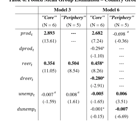
(20) are rather homogeneous and that their wage equation did not change significantly after the break, confirming the fact that the crisis had a smaller impact on the labor market in those countries (compared to the Periphery). In the case of Periphery, the two Models give quite different results, but the bottom line is the same: wages are more weakly related (compared to the Core) to macroeconomic variables. When using Model 3, productivity is long-run excluded (see Table 3) and the reer has homogeneous coefficients across countries. In Model 6, productivity cannot be excluded – although it is heterogeneous and not significant – and only the unemployment rate enters significantly. 19. Table 6. Pooled Mean Group Estimation – Country Groups Model 3. Model 6. "Core" "Periphery" "Core" "Periphery" 𝑝𝑟𝑜𝑑𝑡. (N = 6). (N = 5). (N = 6). (N = 5). 2.893. ---. 2.682. (13.61). ---. (7.24). -0.698 (-0.36). -0.294a. ---. (-1.10). ---. a. -----. 𝑑𝑝𝑟𝑜𝑑𝑡 𝑟𝑒𝑒𝑟𝑡. 0.354. 0.504. 0.458. (11.05). (8.54). (8.26). 𝑑𝑟𝑒𝑒𝑟𝑡 𝑢𝑛𝑒𝑚𝑝𝑡. a. -0.007 (-1.59). a. 0.008 (1.61). 𝑑𝑢𝑛𝑒𝑚𝑝𝑡. 19. a. a. -0.280. ---. (-2.91). ---. -0.005. 0.006. (-1.65). (3.51). -0.001a. -0.007. (-0.15). (-6.69). As shown in the Appendix Table A4, productivity enters the wage equation significantly only for. Italy.. 19.

(21) 𝑒𝑐𝑚𝑡−1. -0.235. -0.162. (-5.20). (-4.10). -0.350. -0.139. (-6.92). (-3.23). a. Note: Dependent variable: waget. t-Students in parentheses. indicates that the corresponding variable was not subject to the restriction of equal long-run parameters for all the members of the group. Thus, its estimate is the Mean Group Estimate, instead of the PMGE.. Table 6 reports the point estimates of the long-run wage equation specified according to the restrictions imposed in Table 5. When looking at the point estimates of the coefficients, we note that the coefficient for productivity in the Core is very large; at the same time, unemployment enters the equation in the two groups with opposite sign. In particular, until the crisis, in the Periphery higher unemployment was associated to higher wages, but this pattern was reversed since the crisis (the coefficient of 𝑑𝑢𝑛𝑒𝑚𝑝 is negative and significant and larger in absolute value), possibly pointing to the role of flexibility-enhancing reforms introduced in particular in Spain, Portugal and Italy in the second period. In both specifications, the error correction term is higher for Core countries, and this is broadly confirmed by the country-specific estimates,20 implying that, when disequilibrium in the labor market occurs, wages adjust more quickly in the Core than in the Periphery. As we acknowledged in Section 2, the proposed specification might present endogeneity issues, in particular as far as the 𝑟𝑒𝑒𝑟 is concerned. For this reason, as a robustness check as in Camarero et al. (2016), we also performed our analysis using the nominal effective exchange rate (𝑛𝑒𝑒𝑟) in place of the real one. 21. 20. See Table A4 in Appendix 1.. 21. While we acknowledge that what matters for competitiveness is actually not the nominal exchange. rate, but rather the real exchange rate, due to price stickiness, movements in the real exchange rate in the short-medium run are driven by nominal exchange rate developments. Moreover, within our sample. 20.

(22) The results, which we do not report here for reasons of space, confirm those obtained using the real exchange rate. 22 6. Concluding remarks This paper investigated differences in wage determination among several EMU member states using panel cointegration techniques that allow for regime shift and coefficient heterogeneity. Our results suggest that the determination of wages in the EMU-11 countries may have been affected by a structural change contemporaneous to the international financial crisis. First of all, we have estimated a common wage equation for the EMU. However, statistical tests on cross-country homogeneity of the long-run coefficients showed that significant heterogeneity is present. The only variable for which country homogeneity could not be rejected was the real exchange rate. The sign is positive, implying that the appreciation of the real exchange rate tended to increase wages in the area, worsening competitiveness. In order to find more homogeneous wage determination models, we have splitted the EMU-11 into two groups of countries that we called, for convenience, “Core” and “Periphery”. Two different adjustment models emerge from the analysis of heterogeneity among the panel members: the Core countries have more homogeneous behavior; moreover, wages in this region significantly respond to macroeconomic conditions (i.e. labor productivity, real exchange rates and. there is a relatively strong positive correlation between the two variables (about 0.5). Finally, while nominal exchange rate developments, affecting the real exchange rate, may in principle affect the real wage, it can hardly be argued that the reverse is true. 22. Results of the analysis using the neer are available from the authors upon request.. 21.

(23) unemployment). In contrast, for Periphery countries, wages are not long-run related to productivity growth and are only negatively related to unemployment (as one would expect) since the regime break of the global financial crisis. These results have important implications. First of all, we had discussed that a number of descriptive indicators suggest that labor markets in the Core appeared to be more dynamic and efficient. The results of the estimation seem to corroborate this hypothesis. The apparent sluggishness of Periphery labor markets, on the other hand, might be related to their weak links to macroeconomic fundamentals. In this respect, this analysis complements the results complement the ones in Camarero et al. (2016) which showed the wage-moderating role of flexible labor markets. Moreover, while the focus of this paper is wage determination, the broad conclusions support the results of Sapir (2006) related to the differences across EU social and labor market models in terms of efficiency and equity. Secondly, these results are important in the perspective of the single monetary policy in the EMU. As discussed in Section 1, heterogeneity in the functioning of labor markets in the euro area is a potential source of asymmetric shocks and/or asymmetric response to a common shock. We have proved that this heterogeneity is indeed present, and this is the case also after the crisis. While, as it has been highlighted also in the policy discourse in the EMU, there cannot be a "one-size-fitsall" in a Monetary Union with very diverse economic characteristics and even stages of development;23 achieving the cyclical convergence which is necessary to maximize. 23. European Commission (2017).. 22.

(24) the effectiveness of the single monetary policy will require policy action or the availability of policy tools to compensate for this heterogeneity 24.. References Alesina, A. and Perotti, R. (1997) "The welfare state and competitiveness", American Economic Review 87(5), pp.921-939. Arpaia, A. and Pichelmann, K. (2007) “Nominal and real wage flexibility in EMU”, European Economy Economic Papers no. 281. Baltagi, B.H.; Blien, U. and Wolf, K. (2000), "The East German wage curve 19931998", Economic Letters 69, pp.25-31. Banerjee, A., Carrion-i-Silvestre, J.L. (2013) Cointegration in panel data with breaks and cross-section dependence. Journal of Applied Econometrics, DOI: 10.1002/jae.2348. Bell, B., Nickell, S. and Quintini, G. (2002) “Wage equations, wage curves and all that”. Labour Economics 9 (3), 341-360. Boeri, T. (2002) ‘Let Social Policy Models Compete and Europe Will Win’. Paper presented at a Conference hosted by the Kennedy School of Government, Harvard University, 11–12 April 2002. Brischoux, M., A. Jaubertie, C. Gouardo, P. Lissot, T. Lellouch and A. Sode (2014): “Mapping out the options for a European minimum wage standard”, TrésorEconomics No. 133, July. Buti M. and Turrini, A. (2015) "Three waves of convergence. Can Eurozone countries start growing together again?", http://voxeu.org/article/types-ez-convergencenominal-real-and-structural Camarero, M., D’Adamo, G. and Tamarit, C. (2016): “The role of institutions in explaining wage determination in the Eurozone: A panel cointegration approach”. International Labour Review, Vol. 155, No. 1, 25-53. Campa, J. M., and L. S. Goldberg (2001) “Employment Versus Wage Adjustment and the U.S. Dollar,” The Review of Economics and Statistics 83(3), 477–89. Chevreux, M. and C. Darmaillacq (2014): “Unionization in France: paradoxes, challenges and outlook”, Trésor-Economics, No. 129, May.. 24. One example that is being discussed in this sense is the creation of a macroeconomic stabilization. function for the euro area.. 23.

(25) European Commission (2016), Report on the euro area, SWD (2016) 391. European Commission (2017): “Reflection paper on the Deepening of the Economic and Monetary Union”, COM(2017) 291, 31 May 2017. ECB (2012) "Euro area labor markets and the crisis", Structural Issues Report, October 2012. Ferrera, M. (1998) ‘The Four “Social Europes”: Between Universalism and Selectivity’. In Rhodes, M. and Meny, Y. (eds) The Future of European Welfare: A New Social Contract? (Basingstoke: Macmillan). IMF (2014) "Youth unemployment in Europe: Okun’s law and beyond" IMF Country Report No. 14/199. Juselius, K. (2006) The Cointegrated VAR Model: Methodology and Applications, Oxford University Press, Oxford. Marcellino, M. and Mizon, G.E. (2001), "Small-system modelling of real wages, inflation, unemployment and output per capita in Italy 1970-1994", Journal of Applied Econometrics vol. 16(3), pages 359-370. Nickell, S.J. (1998) “Unemployment: questions and some answers”, The Economic Journal 108, 802-816. Nunziata, L., (2005) “Institutions and wage determination: a multi-country approach” Oxford Bulletin of Economics and Statistics 67(4), 435-466. OECD (2004) OECD Economic Surveys – Euro area. Pesaran, M. H., Shin, Y. and Smith, R.(1999) “Pooled mean group estimator of dynamic heterogeneous panels” Journal of the American Statistical Association 94, 621-634. Pesaran, M.H. and R. Smith (1995): “Estimating long-run relationships from dynamic heterogeneous panels”, Journal of Econometrics 68, 79-113. Robertson, R. (2003) “Exchange Rates and Relative Wages: Evidence from Mexico,” North American Journal of Economics and Finance 14, 25–48. Sapir, A. (2006) ‘Globalization and the Reform of European Social Models. JCMS, Vol. 44, No. 2, pp. 369–90.. 24.

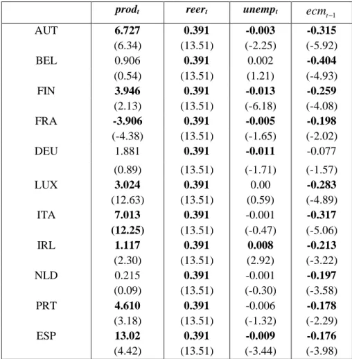
(26) Appendix 1. Individual country estimates a. EMU-11 Table A1. Model 3 AUT BEL FIN FRA DEU LUX ITA IRL NLD PRT ESP. prodt. reert. unempt. ecmt −1. 6.727 (6.34) 0.906 (0.54) 3.946 (2.13) -3.906 (-4.38) 1.881. 0.391 (13.51) 0.391 (13.51) 0.391 (13.51) 0.391 (13.51) 0.391. -0.003 (-2.25) 0.002 (1.21) -0.013 (-6.18) -0.005 (-1.65) -0.011. -0.315 (-5.92) -0.404 (-4.93) -0.259 (-4.08) -0.198 (-2.02) -0.077. (0.89) 3.024 (12.63) 7.013 (12.25) 1.117 (2.30) 0.215 (0.09) 4.610 (3.18) 13.02 (4.42). (13.51) 0.391 (13.51) 0.391 (13.51) 0.391 (13.51) 0.391 (13.51) 0.391 (13.51) 0.391 (13.51). (-1.71) 0.00 (0.59) -0.001 (-0.47) 0.008 (2.92) -0.001 (-0.30) -0.006 (-1.32) -0.009 (-3.44). (-1.57) -0.283 (-4.89) -0.317 (-5.06) -0.213 (-3.22) -0.197 (-3.58) -0.178 (-2.29) -0.176 (-3.98). 25.

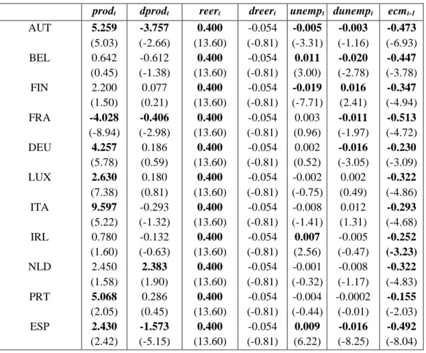
(27) Table A2. Model 6 prodt 5.259 (5.03) 0.642 (0.45) 2.200 (1.50) -4.028 (-8.94) 4.257 (5.78) 2.630 (7.38) 9.597 (5.22) 0.780 (1.60) 2.450 (1.58) 5.068 (2.05) 2.430 (2.42). AUT BEL FIN FRA DEU LUX ITA IRL NLD PRT ESP. dprodt -3.757 (-2.66) -0.612 (-1.38) 0.077 (0.21) -0.406 (-2.98) 0.186 (0.59) 0.180 (0.81) -0.293 (-1.32) -0.132 (-0.63) 2.383 (1.90) 0.286 (0.45) -1.573 (-5.15). reert 0.400 (13.60) 0.400 (13.60) 0.400 (13.60) 0.400 (13.60) 0.400 (13.60) 0.400 (13.60) 0.400 (13.60) 0.400 (13.60) 0.400 (13.60) 0.400 (13.60) 0.400 (13.60). dreert -0.054 (-0.81) -0.054 (-0.81) -0.054 (-0.81) -0.054 (-0.81) -0.054 (-0.81) -0.054 (-0.81) -0.054 (-0.81) -0.054 (-0.81) -0.054 (-0.81) -0.054 (-0.81) -0.054 (-0.81). unempt dunempt -0.005 -0.003 (-3.31) (-1.16) 0.011 -0.020 (3.00) (-2.78) -0.019 0.016 (-7.71) (2.41) 0.003 -0.011 (0.96) (-1.97) 0.002 -0.016 (0.52) (-3.05) -0.002 0.002 (-0.75) (0.49) -0.008 0.012 (-1.41) (1.31) 0.007 -0.005 (2.56) (-0.47) -0.001 -0.008 (-0.32) (-1.17) -0.004 -0.0002 (-0.44) (-0.01) 0.009 -0.016 (6.22) (-8.25). b. "Core" vs. "Periphery" Table A3. Model 3 Countries. prodt. AUT. 2.893 (13.62) 2.893 (13.62) 2.893 (13.62) 2.893 (13.62) 2.893 (13.62) 2.893 (13.62). BEL FIN DEU LUX NLD. Core (N=6) reert 0.354 (11.05) 0.354 (11.05) 0.354 (11.05) 0.354 (11.05) 0.354 (11.05) 0.354 (11.05). Continues in next page. 26. unempt. ecmt −1. -0.039 (-1.13) 0.009 (2.54) -0.017 (-12.38) -0.014 (-2.88) 0.00 (-0.02) -0.015 (-2.63). -0.157 (-4.11) -0.295 (-4.51) -0.364 (-5.01) -0.107 (-2.98) -0.338 (-5.44) -0.147 (-2.80). ecmt-1 -0.473 (-6.93) -0.447 (-3.78) -0.347 (-4.94) -0.513 (-4.72) -0.230 (-3.09) -0.322 (-4.86) -0.293 (-4.68) -0.252 (-3.23) -0.322 (-4.83) -0.155 (-2.03) -0.492 (-8.04).

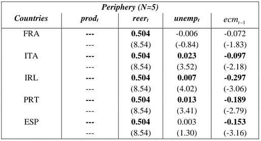
(28) Continues from previous page. Countries FRA. Periphery (N=5) prodt reert ---------------------. ITA IRL PRT ESP. 0.504 (8.54) 0.504 (8.54) 0.504 (8.54) 0.504 (8.54) 0.504 (8.54). unempt. ecmt −1. -0.006 (-0.84) 0.023 (3.52) 0.007 (4.02) 0.013 (3.41) 0.003 (1.30). -0.072 (-1.83) -0.097 (-2.18) -0.297 (-3.06) -0.189 (-2.79) -0.153 (-3.16). Note: Dependent variable: waget. t-Students in parenthesis. Significant coefficients (at 5percent) in bold.. Table A4. Model 6 Core (N=6) Countries Austria Belgium Finland Germany Luxembourg Netherlands. Countries France Italy Ireland Portugal Spain. prodt 2.682 (7.23) 2.682 (7.23) 2.682 (7.23) 2.682 (7.23) 2.682 (7.23) 2.682 (7.23). dprodt -1.384 (-0.77) -0.376 (-0.79) 0.013 (0.03) 0.100 (0.27) -0.606 (-1.37) 0.491 (1.22). reert 0.480 (8.85) 0.642 (4.99) 0.461 (3.54) 0.527 (5.19) 0.401 (6.10) 0.236 (3.68). dreert -0.280 (-2.91) -0.280 (-2.91) -0.280 (-2.91) -0.280 (-2.91) -0.280 (-2.91) -0.280 (-2.91). Periphery (N=5) prodt unempt -7.95 0.006 (-1.33) (3.51) 2.91 0.006 (2.19) (3.51) -0.196 0.006 (-0.19) (3.51) -0.672 0.006 (-0.38) (3.51) 2.417 0.006 (1.44) (3.51). unempt -0.006 (-4.04) 0.003 (0.85) -0.020 (-13.17) -0.003 (-0.58) -0.0005 (-0.18) -0.004 (-1.03). dunempt -0.007 (-6.68) -0.007 (-6.68) -0.007 (-6.68) -0.007 (-6.68) -0.007 (-6.68). dunempt 0.004 (2.43) -0.007 (-1.18) 0.018 (3.48) -0.019 (-1.90) -0.003 (-0.61) -0.003 (-0.74). ecmt-1 -0.430 (-5.75) -0.461 (-5.18) -0.455 (-6.10) -0.146 (-2.30) -0.280 (-4.06) -0.325 (-4.45). ecmt-1 -0.053 (-1.21) -0.170 (-2.82) -0.116 (-2.05) -0.066 (-1.20) -0.291 (-4.26). Note: Dependent variable: waget. t-Students in parenthesis. Significant coefficients (at 5percent) in bold.. 27.

(29) Appendix 2. Detailed variables definition and data sources 𝑢𝑛𝑒𝑚𝑝 𝑐𝑜𝑚𝑝_𝑒𝑚𝑝 𝑒𝑚𝑝_𝑝 𝑟𝑒𝑒𝑟 𝑛𝑒𝑒𝑟 𝑊𝐶𝑂𝑂𝑅. 𝐸𝑃𝐿 𝑟_𝑐𝑜𝑚𝑝 𝑝𝑟𝑜𝑑 𝑈𝐷. unemployment rate. Source: Eurostat. total compensation of employees. Source: Eurostat. thousands of persons employed. Source: Eurostat. ULC-deflated real effective exchange rate. Source: IFS. Nominal Effective Exchange Rate. Source: Eurostat. Coordination of wage bargaining. 5: economy-wide bargaining; 4: mixed industry- and economy-wide; ... 1= company-level bargaining. Source: ICTWSS Database. Employment Protection Legislation. 0 = minimum employment protection; 5 = maximum employment protection. Source: OECD. real compensation per employee: ln(𝑐𝑜𝑚𝑝_𝑒𝑚𝑝) – ln(𝑒𝑚𝑝_𝑝) – ln(𝐶𝑃𝐼). CPI is seasonally adjusted using TRAMO/SEATS. labor productivity per worker: ln(𝑔𝑑𝑝) – ln(𝑒𝑚𝑝_𝑝) union density (in percent). Source: ICTWSS Database.. 28.

(30)