Electro- and magnetostatics of topological insulators as modeled by planar,
spherical, and cylindrical
θ
boundaries: Green
’
s function approach
A. Martín-Ruiz,1,*M. Cambiaso,2 and L. F. Urrutia1
1Instituto de Ciencias Nucleares, Universidad Nacional Autónoma de México, 04510 México, Distrito Federal, Mexico
2Universidad Andres Bello, Departamento de Ciencias Fisicas, Facultad de Ciencias Exactas, Avenida Republica 220, Santiago, Chile
(Received 30 November 2015; published 17 February 2016)
The Green’s function method is used to analyze the boundary effects produced by a Chern-Simons extension to electrodynamics. We consider the electromagnetic field coupled to aθterm that is piecewise constant in different regions of space, separated by a common interfaceΣ, theθboundary, model which we will refer to asθelectrodynamics. This model provides a correct low-energy effective action for describing topological insulators. Features arising due to the presence of the boundary, such as magnetoelectric effects, are already known in Chern-Simons extended electrodynamics, and solutions for some experimental setups have been found with a specific configuration of sources. In this work we construct the static Green’s function inθelectrodynamics for different geometrical configurations of theθboundary, namely, planar, spherical and cylindricalθ-interfaces. Also, we adapt the standard Green’s theorem to include the effects of theθboundary. These are the most important results of our work, since they allow one to obtain the corresponding static electric and magnetic fields for arbitrary sources and arbitrary boundary conditions in the given geometries. Also, the method provides a well-defined starting point for either analytical or numerical approximations in the cases where the exact analytical calculations are not possible. Explicit solutions for simple cases in each of the aforementioned geometries forθboundaries are provided. On the one hand, the adapted Green’s theorem is illustrated by studying the problem of a pointlike electric charge interacting with a planar topological insulator with prescribed boundary conditions. On the other hand, we calculate the electric and magnetic static fields produced by the following sources: (i) a pointlike electric charge near a sphericalθboundary, (ii) an infinitely straight current-carrying wire near a cylindrical θ boundary and (iii) an infinitely straight uniformly charged wire near a cylindrical θ boundary. Our generalization, when particularized to specific cases, is successfully compared with previously reported results, most of which have been obtained by using the method of images.
DOI:10.1103/PhysRevD.93.045022
I. INTRODUCTION
It is not seldom that seemingly abstract mathematical models find widespread application in several fields of theoretical as well as applied physics. A paramount example of this is Einstein’s theory of general relativity, because in order to achieve the accuracy that render GPSs useful, relativistic effects must be taken into account. Filling the gap from theory to applied engineering is only a matter of time. Fortunately, the time span from conception to application gets shorter and shorter. So is the case with the study of Chern-Simons (CS) forms [1] to its applica-tions in topological insulators, spintronics and topological quantum computer science [2,3].
The relevance of CS forms also is apparent in theoretical physics. In quantum field theories, they play a prominent role in regard to anomalies. The existence of anomalies can jeopardize the consistence of the theory as they would be indicative of gauge symmetry violation, hence the need for
mediated bySUð2Þinstantons (sphalerons) can transmute leptons into baryons under certain conditions that would have been met during the out-of-equilibrium inflationary epoch of the Universe [7,8].
In a very simple guise, CS terms were used by Peccei and Quinn by the introduction of the axion in order to solve the strong CP problem of QCD [9]. Soon after ’t Hooft realized that the unobservedUð1Þ symmetry of QCD can be understood due to the dynamics of instantons [10]. Wilczek explicitly predicted applications of axion-electrodynamics to the field of material science [11]. Further studies involve its uses in topological quantum field theory [12], topological string theory [13] and as a quantum gravity candidate [14].
In this work we will be concerned with a simple case of CS theories, akin to axion-electrodynamics, introduced by Wilczek as mentioned above in the context of particle physics. We will refer to this particular model as
θ-electrodynamics or simply θ ED, and it amounts to extending Maxwell electromagnetism by a gauge invariant term of the form
ΔLθ¼θðα=4π2ÞE·B: ð1Þ Here though, θis no longer a dynamical field, but rather we take it as a constant, a genuine Lorentz scalar, and thus Eq. (1) is a pseudoscalar. Written in a manifestly covariant way
ΔLθ ¼−θ4ðα=4π2ÞFμνF~μν; ð2Þ
the identification with the Pontryagin invariant associated with theUð1Þgauge connectionA¼Aμdxμis immediate. In the latter we introduced the Hodge dual field strength electromagnetic tensor F~μν¼12ϵμναβFαβ, and ϵμναβ is the Levi-Civitá symbol.
The idea ofθED has been studied in several situations and also extrapolated to study other systems. In other contexts,θED under consideration here has been studied as a3þ1particular kind of Maxwell-Chern-Simons electro-dynamics, where it has received considerable attention [15–31]. And also it has been studied as a restricted subset of the Standard Model extension [32,33], where several results have been achieved, too[34–40].
Further, the topological nature of theθ term of Eq. (2) can be seen by the fact that this CS extension is a total derivative. Therefore, it produces no contribution to the field equations of motion when usual boundary conditions are met; the contribution is a boundary term that vanishes whenever one imposes the vanishing of the fields at the boundary (or at infinity in the case the theory is defined over the whole space). Shouldθcease to be a constant in the manifold where the theory is defined, the CS term would fail to be a topological invariant, and therefore the
corresponding modifications to the field equations would need to be taken into consideration.
In this paper, we will be concerned with the simplest nontrivial case in this context; namely, we will study the modifications to Maxwell’s theory defined on a manifold in which either (a) there are two domains defined by their different constant values of θ, i.e., θ is space dependent
θðxÞ, or (b) there is a nonvanishing θ value and the manifold has a boundary where the fields or their deriv-atives are not vanishing, with either Dirichlet or Neumann boundary conditions. A constantθcan be thought of as an effective parameter characterizing properties of a novel electromagnetic vacuum, possibly arising from a more fundamental theory, where discontinuities in the value of
θhas interesting properties. This approach has been taken in the context of classicalθED[41–44]and in the context of quantum vacuum[45]. A similar avenue has been taken in the context of Janus field theories[46–51]. These were motivated from the gravitational sector of the AdS/CFT correspondence, by an exact and nonsingular solution for the dilatonic field in type IIB supergravity [52]. The similarity is due to the fact that the coupling constant of the ensuing four-dimensional N ¼4 super Yang-Mills theory living in the boundary exhibits a spacetime depen-dent character. For further insight on the similarities and differences between Janus field theories and θ ED as studied in this work, see Ref.[53]and references therein. On the other hand, as applied to material media,θcan be regarded as an effective macroscopic parameter to describe new degrees of freedom of quantum matter. This approach has been thoroughly used in the context of topological insulators (TIs) as will be explained below.
First, recall that in general CS forms are amenable for capturing topological features of the physical system that they describe. Formally, this can be seen from the action principle. Given a symmetry group and an odd-dimensional differentiable manifold where fields and functions are defined, a gauge connection one-form can be defined of which the associated curvature two-form can be used to build 2k-forms that (i) are gauge invariant under the symmetry group, (ii) are closed and therefore expressible in terms of a (2k−1)-form and (iii) the integral of which is a topological invariant. This last point is crucial revealing the importance of boundaries. Its many uses in gravitation and the former description are clearly reviewed in Ref.[54]. The latter description is tailor made for the understand-ing of what came to be known as topological phases. The discovery of the quantum Hall (QH) state made manifest the existence of new states of matter that do not fall into Landau-Ginzburg’s effective field theory paradigm. In it, the quantum mechanical states of matter that determine the different phases are characterized by the spontaneous breaking of a global symmetry of the quantum mechanical system. Von Klitzing’s discovery of the astonishing pre-cision with which the Hall conductance of a sample is
quantized [55], despite the varying irregularities of the sample, turned out to have a topological origin. The ensuing electric current along the edge of a 2D electron gas at very low temperature, due to an external magnetic field applied perpendicular to the sample, is in fact insensitive to the sample’s geometric details. The reason for this lies in the band structure of the sample. For the QH state, the system is insulating in the bulk and conducting in the boundary. The Hamiltonian of the many-particle system in the bulk exhibits an energy gap separating the ground state from the excited states. On the contrary, for the edge states, the band structure is gapless. Furthermore, one can define a smooth deformation in the Hamiltonian parameter space (the symmetry transformation referred to in the previous paragraph, the transformation taking the coffee mug to a torus) that does not close the bulk gap. To finally understand the connection with topology, one can recall the Gauss-Bonnet formula and Berry’s phase, the generaliza-tion of the concept of curvature to quantum mechanical systems. The former allows one to express the genusgof a surfaceSin terms of an integral over the local curvature of the surface. The latter is a measure of the phase accumu-lated by a wave function as it evolves under a slow and closed variation in the parameter space of the Hamiltonian. Back in the QH scenario, the Hall conductance can be expressed as an invariant integral over the frequency momentum space, more precisely as an integral of the Berry curvature over the Brillouin zone[56]. This quantity plays the role of a topological order parameter uniquely determining the nature of the quantum state inasmuch as the order parameter in Landau-Ginzburg effective field theory determines the usual phases of quantum matter.
As mentioned previously, CS terms lend themselves for the description of topological features of a given physical system. Concretely, in material science systems, the low-energy limit of the electrodynamics of topological insulators can be described by extending Maxwell electro-dynamics precisely by the θ term of Eq. (2), originally formulated in4þ1dimensions but appropriately adapted to lower dimensions by dimensional reduction[57]. Thus,θ ED as a topological field theory serves as model for many theoretical[58–60]and experimental realizations for study-ing detailed properties of topological states of quantum matter[2,41,61,62]. See also the review papers[63,64]and references therein.
The general scope of this work is to introduce Green’s function (GF) methods inθ ED, which are well suited to deal with the calculation of electric and magnetic fields arising from arbitrary sources, as well as to solve problems with given Dirichlet or Neumann boundary conditions on arbitrary surfaces. This approach is more general than the method of images which, to our knowledge, has been systematically employed in most of the previous works on the related literature. On the other hand, the GF method provides a precise starting point from where either
analytical or numerical approximations can be performed. In Ref.[53], we have already presented the first steps in this direction by constructing the GF for a θ boundary with planar geometry. The method was applied to the calculation of some specific examples. The GF for a stack of layered time-reversal-symmetry-broken TIs has been constructed in Ref.[65]and applied to describe novel field patterns arising from the magnetoelectric effect due to a dipole close to the surface of the TI.
The paper is organized as follows. In Sec.II, we review the basics of Chern-Simons electrodynamics defined on a four-dimensional spacetime characterized by a piecewise constant value ofθin different regions of space separated by a common boundary Σ. To isolate the effects of the θ term on the GFs and of the stress-energy tensor, we will take the media on either side of theΣ boundary with no dielectric nor magnetic properties, i.e., ϵ¼1 and μ¼1 across Σ. Including electric and magnetic susceptibility properties proceeds accordingly. We will restrict our analysis to the case of electro- and magnetostatics. As in usual Maxwell electrodynamics, a robust static theory is necessary and important to understand the dynamical case as well as the ensuing quantum electrodynamics. In this scenario, the field equations remain the standard Maxwell equations in the bulk, but the discontinuity ofθ modifies the behavior of the fields at the interface Σ. The most striking feature of this theory is that even in the static limit, electric and magnetic fields are intertwined. Aspects about a possibility to circumvent Earnshaw’s theorem and how to obtain the modified conservation laws are revised; in particular, a detailed construction of the stress-energy tensor is presented.
In Sec. III, we start by adapting Green’s theorem to incorporate the contributions of theθboundary. Also, we classify the different boundary conditions that can be imposed there. Restricting ourselves to the case where we do not impose boundary conditions at theθ interface (i.e., boundary conditions only at infinity), we consider the simplest geometries for the Σ: planar, cylindrical and spherical. We present a brief review of the planar case and construct the static GF matrix for the remaining geometries, thus providing the general solution to the modified field equations for the case of arbitrary configu-ration of sources. The method can be extended to the case of other geometries, but we focus on these configurations given the fact that those are the ones that have attracted the most of the experimental efforts. This is an important part of our paper. In it, not only do we aim to provide practical solutions for a given boundary-value problem with arbi-trary external sources but also to provide a means to improve the understanding of the theory.
when Dirichlet boundary conditions are imposed on a planar Σ. Also, we discuss other applications, where we make contact between the results obtained with our method and others in the existing literature, a comparison that endorses our approach, for instance, the problem of a pointlike charge near a sphericalθboundary together with the cases of a current-carrying wire and a uniformly charged wire near a cylindrical θ boundary. Finally, in Sec. V, we summarize our results and give further con-cluding remarks. Throughout the paper, Lorentz-Heaviside units are assumed (ℏ¼c¼1), the metric signature will be taken as ðþ;−;−;−Þ, and the convention ϵ0123¼ þ1 is adopted.
II. θELECTRODYNAMICS IN A BOUNDED REGION
A. Field equations and boundary conditions
Let us consider the additional coupling of electrody-namics with the electromagnetic Pontryagin invariant
P¼FμνF~μν; ð3Þ
via a scalar fieldθdefined by the action S¼
Z
Md 4x
− 1
16πFμνFμν−
1 4
θðxÞ
2π α
2πFμνF~μν−jμAμ
;
ð4Þ
where α¼e2=ℏc is the fine structure constant, F~μν¼
1
2ϵμναβFαβ is the dual of the field strength tensor andjμis a conserved external current. The coupling constant for theθ term, α=4π2, is chosen in such a way that the Dirac quantization condition for the magnetic charge be an integer multiple of e=2α, as discussed in Ref. [11]. The topological nature of the Pontryagin density makes the equations of motions arising from the action (4)invariant under the change θðxÞ→θðxÞ þC, with C any constant. Quantum mechanical arguments impose further conditions onC, which will be discussed in the following.
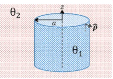
The (3þ1)-dimensional spacetime is M¼U×R, where U is a three-dimensional manifold and R corre-sponds to the temporal axis. We make a partition of space in two regions,U1 andU2, in such a way that manifoldsU1 andU2 intersect along a common two-dimensional boun-dary Σ, to be called the θ boundary, so that U¼U1∪U2 andΣ¼U1∩U2, as shown in Fig.1. We also assume that the fieldθis piecewise constant in such way that it takes the constant valueθ¼θ1in regionU1and the constant value
θ¼θ2 in region U2. This situation is expressed in the characteristic function
θðxÞ ¼ θ
1; x∈U1
θ2; x∈U2
: ð5Þ
In this scenario, theθterm in the action fails to be a global topological invariant because it is defined over a region with the boundaryΣ. Varying the action gives rise to a set of Maxwell’s equations with an effective additional current with support at the boundary
∂μFμν¼θδ~ ðΣÞnμF~μνþ4πjν; ð6Þ
wherenμ¼ ð0;nÞ,nis the outward unit normal to Σand ~
θ¼α
πðθ1−θ2Þ: ð7Þ
Current conservation can be verified directly by taking the divergence at both sides of Eq. (6),
∂ν∂μFμν¼θδ~ 0ðΣÞnμnνF~μνþθδ~ ðΣÞnμ∂νF~μνþ4π∂νjν; ð8Þ
where the left-hand side and the first two terms in the right-hand side vanish due to symmetry properties.
Together with the Bianchi identity∂μF~μν¼0, the set of Eqs.(6)forθED can be written in coordinates adapted to the surface as
∇·E¼θδ~ ðΣÞB·nþ4πρ; ð9Þ
∇×B−∂E
∂t ¼θδ~ ðΣÞE×nþ4πJ; ð10Þ
∇·B¼0; ð11Þ
∇×Eþ∂B
∂t ¼0; ð12Þ
wheren is the unit normal to Σshown in Fig. 1. In this work, we consider the simplest geometries corresponding to the cases where the surfaceΣ is taken as (i) the plane
z¼a, (ii) a sphere with center at the origin and radius a
and (iii) an infinitely straight cylinder of radiusawith axis parallel to the z direction. In these cases, the choice of adapted coordinates has an obvious meaning: (i) Cartesian coordinates, (ii) spherical coordinates and (iii) cylindrical coordinates, respectively.
As we see from Eqs.(9)–(12) the behavior ofθ ED in the bulk regions U1 and U2 is the same as in standard
FIG. 1. Region over which the electromagnetic field theory is defined.
electrodynamics. Theθterm modifies Maxwell’s equations only at the surface Σ. Here, Fi0¼Ei, Fij¼−εijkBk and
~
Fi0¼Bi, F~ij ¼εijkEk. Equations (9)–(12) also suggest that the electromagnetic response of a system in the presence of a θ term can be described in terms of Maxwell equations in matter
∇·D¼4πρ; ∇×H¼4πJ; ð13Þ
with constitutive relations D¼Eþα
πθðxÞB; H¼B− α
πθðxÞE; ð14Þ
where θðxÞ is given in Eq. (5). It is clear that ifθðxÞ is globally constant in M, there is no contribution to Maxwell’s equations from the θ term in the action, even thoughθðxÞstill is present in the constitutive relations. In fact, the additional contributions of a globally constantθðxÞ to each of the equations (13) cancel due to the homo-geneous equations(11)and (12).
So far we have consideredθas an external parameter that can take arbitrary values, albeit respecting the rescaling symmetryθ→θþCthat we already mentioned. Naively, this would allow one to setθto zero at the classical level. However, quantum mechanically, given that for properly quantized electric and magnetic fluxesSθ=ℏis an integer multiple ofθ, then the only allowed values of CareC¼
2πnfor integern; otherwise, nontrivial contributions to the path integral would result. The above argument together with additional considerations about the behavior of the system under time reversal (TR) can further constrainθ. In fact, in the context of TIs, it was originally assumed that only systems with broken TR symmetry are of relevance; however, it was soon realized that systems preserving TR symmetry are as important; see Ref. [66]. Given the pseudoscalar nature under TR of the CS coupling,
TðE·BÞ ¼−E·B, whereT is the time-reversal operator
T∶t→−t, it seems that breaking TR symmetry is inescap-able. However, TR symmetry can be preserved as long asθ takes the values 0 orπ(mod2π). Forθ¼0, the system is trivially TR invariant, whereas forθ¼π, it can be restored by suitably rescaling θ; i.e., TðπE·BÞ ¼−πE·Bcan be made TR invariant by θ→θ0¼θþ2π. For the sake of generality, in the sequel, we will not restrict to systems with a definite TR symmetry property, and therefore the only relevant constraint for θ that we will consider is that its observable effects satisfy theθ→θþ2πnsymmetry,[63]. This property is made self-evident because all our observ-able results will depend only on the combinationθ~ given in Eq.(7).
Assuming that the time derivatives of the fields are finite, in the vicinity of the surfaceΣ, the field equations imply that the normal component ofE, and the tangential components of B, acquire discontinuities additional to those produced by superficial free charges and currents,
while the normal component of B, and the tangential components of E, are continuous. For vanishing external sources onΣ, the boundary conditions read
ΔEnjΣ¼θ~BnjΣ; ð15Þ
ΔB∥jΣ¼−θ~E∥jΣ; ð16Þ
ΔBnjΣ¼0; ð17Þ
ΔE∥jΣ¼0: ð18Þ
The notation isVijzz¼¼aaþ−¼ViðzÞjz¼a
þ
z¼a−¼limϵ→0ðViðz¼aþϵÞ− Viðz¼a−ϵÞÞ, ϵ>0 and Vijz¼a¼Viðz¼aÞ, for any vectorV.
The continuity conditions, Eqs.(17)and(18), imply that the right-hand sides of Eqs.(15)and(16)are well defined and they represent surface charge and current densities, respectively. An immediate consequence of the boundary conditions is that the presence of a magnetic field crossing the surfaceΣis sufficient to generate an electric field, even in the absence of free electric charges. For aθ boundary characterizing different θ values of the electromagnetic vacuum, these issues together with some of its conse-quences over the propagation of electromagnetic waves across such interfaces were studied in Refs. [43,44]. It is worth mentioning that with the modified boundary con-ditions, several properties of conductors in static fields still hold as far as the conductor does not lie in theΣboundary. In particular, conductors are equipotential surfaces, and the electric field just outside the conductor is normal to its surface.
B. Possibility to circumvent Earnshaw’s theorem It is a well-established fact in ordinary electrostatics that, due to electrostatic forces alone, a charge cannot be in stable equilibrium (Earnshaw’s theorem). More generally, no static object comprised of electric charges, magnets and masses can be held in static equilibrium by any combina-tion of electric, magnetic or gravitacombina-tional forces.
−∇2ϕ¼4πρþθδ~ ðΣÞB·n: ð19Þ We inquire whether the potential has an extremum at a pointPwhere a test charge is to be held in equilibrium. The argument proceeds in the usual manner. Suppose that there exists a pointPat whichϕacquires a minimum. Then, at every point over the surface of any small closed surface enclosingP, one must have∂nϕ>0, wherendenotes the outward normal direction to the surface and thus one must have
I
∂V∂nϕds >0; ð20Þ
where the volumeVenclosesP. Due to∂nϕ¼∇ϕ·nand to the divergence theorem, this latter integral can be cast into a volume integral of the Laplacian of the potential. Again, to isolate the contribution due to theθterm, we set
ρ¼0to obtain I
∂V∂nϕds¼ Z
V∇ 2ϕdv
¼−θ~
Z
VδðΣÞB·ndv ¼−θ~
Z
ΣBnjΣd
2x: ð21Þ
In ordinary Maxwell electrostatics (θ~ ¼0), the right-hand side of Eq. (21) vanishes, leading to a contradiction with Eq. (20) and thus proving that P cannot be a local minimum. In the case ofθED, however, as far asθ~ ≠0and a nonvanishing normal magnetic field at Σ exists, the aforementioned contradiction no longer occurs, for points
P at Σ, thus removing the immediate obstruction of ordinary electromagnetism for the existence of local minima. We emphasize that by no means are we claiming to have proven the existence of points of stable equilibrium in θelectrostatics, which can be dealt with elsewhere. To this end, a more thorough analysis is required along the lines of Ref. [67] in the context of ordinary electromag-netism. We consider this an important issue. Charged or magnetized matter can be held in static equilibrium in a given experimental setup. However, if this were possible only with the aid of external devices such as tweezers or dynamical mechanisms or EM traps, e.g., Penning traps [68], these could compromise the precision of the mea-surements or interact with the EM fields under study.
C. Stress-energy tensor
For the case ofθED, we still expect the electromagnetic field to be an energy-momentum transmitting entity. In this way, for example, we should be able to compute the net force over a given region in 3-space in terms of the values of the electromagnetic fields on the bounding surface of
that region. This requires establishing conservation laws, as in ordinary Maxwell electrodynamics. In Sec.II A, we showed that theθterm modifies the behavior of the fields at the surfaceΣonly. This suggests that, for each region in the bulk, the energy-momentum tensor forθED has the same form as that in standard electrodynamics, where the θ~ dependence appears through the contribution to the fields arising from the additional sources present on the boundary Σ. In fact, the identification of the stress-energy tensor proceeds along the standard lines of electrodynamics in a medium (see, for example, Ref.[69]), where we read the rate at which the electric field does work on the free charges
J·E¼−∇·
1 4πE×H
− 1
4π
E·∂D
∂t þH· ∂B
∂t
ð22Þ
and the rate at which momentum is transferred to the charges
ρEþJ×B¼− 1 4π
∂
∂tðD×BÞ−
1
4π½Di∇Ei−∇·ðDEÞ
− 1
4π½Bi∇Hi−∇·ðBHÞ: ð23Þ Here, the notation isAi∇Bi¼ ðAi∂kBiÞˆekand∇·ðABÞ ¼ ð∂iAiÞBkeˆkfor any vectorsAandB. Using the constitutive relations in Eq.(14), we recognize from Eq.(22)the energy fluxS and the energy densityU as
S¼ 1
4πE×B; U¼
1
8πðE2þB2Þ; ð24Þ
while from Eq.(23), we obtain the momentum densityG, and we identify the stress tensorTij as
G¼ 1
4πE×B; Tij¼ 1
8πðE2þB2Þδij− 1
4πðEiEjþBiBjÞ: ð25Þ
Outside the free sources, the conservation equations read
∇·Sþ∂U
∂t ¼0;
∂Gk
∂t þ∂iTik¼ α
πðE·BÞ∂kθðxÞ: ð26Þ
In other words, the stress-energy tensor has in fact the same form as in vacuum, but, as expected, it is not conserved on the θ boundary because of the self-induced charge and current densities arising there.
In the standard case, the knowledge of both the stress-energy tensor together with the GF of the system is also relevant in the quantum situation. For example, when dealing with the calculation of Casimir energies, the
vacuum expectation value of the energy momentum can be obtained with the aid of the corresponding GF for Maxwell electrodynamics [70–72]. Using this method, insights regarding corrections to the Casimir energy in the context ofθED have been developed in Refs.[45,73], as well as Ref.[39]for a related perspective. This approach serves as an additional motivation for the following Sec. III.
III. GREEN’S MATRIX METHOD
In this section, we use the GF method to solve boundary-value problems in θ ED in terms of the electromagnetic potentialAμ. Certainly, one could solve for the electric and magnetic fields from the modified Maxwell equations (9) through (12) together with the boundary conditions in Eqs.(15)–(18); however, just as in ordinary electrodynam-ics, there might be occasions where, besides the knowledge of the external sources, we are provided with requirements on the fields at the given boundaries. In these cases, the GF method provides the general solution to a given boundary-value problem (Dirichlet or Neumann) for arbitrary sources. The importance of such a general solution is evident from an experimental point of view. For example, it would allow one, at least in principle, to predict the electromagnetic response of topological insulators with planar, spherical or cylindrical boundaries in the presence of more intricate configuration of sources. Moreover, as already mentioned in Sec.II C, the GF method is useful for computing the vacuum expectation value of the energy-momentum tensor in the context of Casimir forces. Furthermore, the GF method should be also useful for the solution of dynamical problems inθ ED.
In the following, we concentrate only on the static case. Since the homogeneous Maxwell equations that express the relationship between potentials and fields are not modified in θED, the electrostatic and magnetostatic fields can be written in terms of the 4-potentialAμ¼ ðϕ;AÞaccording to E¼−∇ϕ and B¼∇×A, as usual. In the Coulomb gauge ∇·A¼0, the 4-potential satisfies the equations of motion
½−ημ
ν∇2−θδ~ ðΣÞnαϵαμβν∂βAν¼4πjμ; ð27Þ
together with the boundary conditions (BCs) ΔAμjΣ¼0;
Δðnα∂αAμÞjΣ¼−θ~nαϵαμβν∂βAνjΣ: ð28Þ
Here, nα is the unit normal to Σ, which depends on the geometry of theθboundary. One can further verify that the BCs of Eq. (28) yield those obtained in Eqs. (16)–(18), starting from the modified Maxwell equations.
To obtain a general solution for the potentialsϕandA in the presence of arbitrary external sources jμðxÞ, we
introduce the GF matrixGμνðx;x0Þ, solving Eq.(27)for a pointlike source,
½−ημ
ν∇2−θδ~ ðΣÞnαϵαμβν∂βGνσðx;x0Þ ¼4πημσδ3ðx−x0Þ; ð29Þ
together with the BCs of Eq. (28). In the following, we discuss the general solution to Eq.(29). To this end, we require an appropriate adaptation of the standard Green’s theorem, from which the solution of Eq. (29) can be constructed using well-known methods.
A. Green’s theorem and boundary conditions on Σ
We begin this section by introducing the differential operator
Oμ
νi¼ημν∂iþθδ~ ðΣÞnjϵjμνi; ð30Þ
from which the relationsOμνi∂
iAν¼4πjμandOμνi∂iGνσ¼ 4πημ
σδ3ðx−x0Þ correctly yield the differential equations for the 4-potential in Eq.(27)and the GF in Eq.(29). Here, the indexesi,jrange from 1 to 3, while μ,ν range from 0 to 3. These choices reflect that we are working with static fields and that the normal to the θ boundary is always spacelike.
The relevant Green’s theorem can be given in terms of two arbitrary fields, Xμ and Zμν. Defining the tensor
Ti
σ ¼XμOμνiZνσ, using the divergence theorem for ∂iTiσ and subtracting the equation arising from the inter-changeX↔Z, we find
I
S
dSniðXμOμνiZνσ−ZνσOμνiXμÞ
¼ Z
V
d3x½XμOμνið∂iZνσÞ−ZνσOμνið∂iXμÞ
−
Z
V
d3x½ð∂iXμÞOμνiZν
σ−ð∂iZνσÞOμνiXμ; ð31Þ
wherenis the outward normal to the surfaceSbounding the volume V. In deriving Eq. (31), we use the result ∂iOμ
νi¼Oμνi∂i, which follows directly from Eq.(30). Substituting Eqs.(27)and(29)in Eq.(31), we find that the general solution for the 4-potential in the Coulomb gauge is
AμðxÞ ¼
Z
V
d3x0Gμνðx;x0Þjνðx0Þ
þ 1
4π
I
S
dS0ni½Aνðx0Þ∂iGμνðx;x0Þ
−Gμνðx;x0Þ∂iA νðx0Þ
þ θ~ 4π
Z
Σd
2x0
Σnjϵjανi½Aαðx0Þ∂iGμνðx;x0Þ
wherenjis the normal to theθboundary. This result yields the standard interpretation where the first term is the contribution from the sources inside the volume V, the second term represents the effects of the bounding surface
S, while the remaining term replaces the contributions from the surface Sby those of theθ boundary.
We next consider the issue of the appropriate BCs for the fields at the θ interface, when we take S as a surface at infinity where the usual BCs are imposed. Inspection of Eq.(32)reveals that there are four classes of BCs onΣthat specify a solution.
The class BC-I is defined by fixing, on Σ, the scalar potential A0 and the vector potential parallel to the θ boundary n×A, together with the requirement
njϵjα
νiGμνjΣ¼0onΣ. This class describes the case which
corresponds to the nearest analogy with the standard Dirichlet BCs. Besides, it is the only class for which the explicit GF is independent of the area of theθboundary. In Sec.IV, we solve the problem of a pointlike charge near a planarθ boundary at fixed potential using class BC-I.
The class BC-II is specified by fixing onΣthe normal component of the magnetic field Bn and the parallel component of the electric field n×E, plus the condition
njϵjα
νi∂iGμνjΣ¼1=Aθ, whereAθ ¼ R
d2xΣ is the surface area of the θ boundary. This class corresponds to the Neumann BCs in standard electrostatics, which incorpo-rates a factor of the inverse surface area, generating a term in the solution involving the average contribution of the potential.
The class BC-III fixes the scalar potential A0 and the normal component of the magnetic field Bn on Σ, together with the conditions njϵj0kiGμkjΣ¼0 and njϵjk
0i∂iGμ0jΣ¼1=Aθ.
The class BC-IV requires specifyingn×Aand n×E onΣ. For this class, we must also demandnjϵjk0iGμ0jΣ¼0
andnjϵj0
ki∂iGμkjΣ¼1=Aθ.
In the next subsections, we deal with the problem of constructing the GFs for different geometrical configura-tions of theθboundary, considering those which could be more relevant in experimental works, namely, planar, spherical and cylindrical θ interfaces. Moreover, having set the surfaceS at infinity, with standard BCs there, we restrict ourselves to the case where we do not specify any additional condition for the fields at theθboundary. In this way,Aμis given only by the first term of the right-hand side in Eq.(32).
B. Planar θboundary
For the case of planar symmetry, we choose the simplest setup in which the value ofθjumps across the planeΣand remains constant at either side ofΣ, defined byz¼aand indicated in Fig.2. In this way, the adapted coordinates to this system are the Cartesian ones. The GF we consider has translational invariance in the directions parallel toΣ, that is
in the transverse directionsxandy, but this invariance is broken in the direction z. Exploiting this symmetry, we further introduce the Fourier transform in the direction parallel to the planeΣ, taking the coordinate dependence to beðx−x0Þ∥¼ ðx−x0; y−y0Þ, and define
Gμνðx;x0Þ ¼4π
Z
d2p
ð2πÞ2eip·ðx−x 0Þ
∥gμνðz; z0;pÞ; ð33Þ
wherep¼ ðpx; pyÞis the momentum parallel to the plane Σ. In the following, we suppress the dependence onpof the reduced GFgμν. In this case, the reduced GF satisfies
½∂2ημ
νþiθδ~ ðz−aÞϵ3μανpαgνσðz; z0Þ ¼ημσδðz−z0Þ; ð34Þ
where ∂2¼p2−∂2z, pα¼ ð0;pÞ and p2¼−pαpα¼
p2xþp2y. The solution of Eq. (34) is a simple, but not straight-forward, task. For solving it, we employ a method similar to that used for obtaining the GF for the one-dimensional δ-function potential in quantum mechanics, where the free-particle GF is used for integrating the GF equation with the δ-interaction. A main simplification arises in this case because what normally results in an integral equation reduces to an algebraic equation in virtue of the fact that the integration over theδ-potential can be performed. To proceed in an analogous way, we consider the reduced free GF having the form Gμ
νðz; z0Þ ¼gðz; z0Þημν, which solves the equation ∂2Gμ
νðz; z0Þ ¼ημνδðz−z0Þ: ð35Þ
The details of the calculation for solving Eq. (34) were presented in Ref. [53]. For completeness, we remind the reader of the general solution
gμνðz; z0Þ ¼ημνgðz; z0Þ−θ~ gðz; aÞgða; z
0Þ
1þp2θ~2g2ða; aÞ
×fθ~gða; aÞ½pμpνþ ðημνþnμnνÞp2
þiϵμνα3pαg; ð36Þ
wherenμ¼ ð0;0;0;1Þ is the normal toΣ.
The reciprocity between the position of the unit charge and the position at which the GF is evaluated
FIG. 2. Geometry of the semi-infinite planar θ-region.
Gμνðx;x0Þ ¼Gνμðx0;xÞ is one of its most remarkable properties. From Eq. (33), this condition requires
gμνðz; z0;pÞ ¼gνμðz0; z;−pÞ; ð37Þ
which we verify directly from Eq. (36). The symmetry
gμνðz; z0Þ ¼gνμðz; z0Þ ¼g†μνðz; z0Þ is also manifest. The various components of the static GF matrix in coordinate representation were obtained by Fourier transforming the reduced GF, as defined in Eq. (33). In vacuum, with no additional boundaries, the reduced GF is gðz; z0Þ ¼ e−pjz−z0j=2p, and the corresponding GF matrix in coordi-nate representation is (see Ref. [53])
G00ðx;x0Þ ¼ 1
jx−x0j− ~
θ2 4þθ~2
1 ffiffiffiffiffiffiffiffiffiffiffiffiffiffiffiffi
R2þZ2
p ; ð38Þ
G0iðx;x0Þ ¼− 2~θ
4þθ~2 ϵ0ij3Rj
R2
1− ffiffiffiffiffiffiffiffiffiffiffiffiffiffiffiffiZ
R2þZ2
p
; ð39Þ
Gijðx;x0Þ ¼ηijG00ðx;x0Þ−
i
2 ~
θ2
4þθ~2∂iKjðx;x0Þ; ð40Þ
where Z¼ jz−aj þ jz0−aj, Rj¼ ðx−x0Þj
∥¼ ðx−x0; y−y0Þ,R¼ jðx−x0Þ∥jand
Kjðx;x0Þ ¼2i
ffiffiffiffiffiffiffiffiffiffiffiffiffiffiffiffi
R2þZ2
p
−Z R2 R
j: ð41Þ
Finally, we observe that Eqs. (38)–(40) contain all the required elements of the GF matrix, according to the choices of zandz0 in the function Z.
C. Sphericalθ boundary
In the preceding section, the problem of an arbitrary charge and current distributions in the presence of a planeθ boundary was discussed by the method of GF matrix. In this section, following the same procedure as in the planar situation, we discuss the spherical case, in which the value of θ has a discontinuity across the surface r¼a. In the adapted spherical coordinatesr,ϑ,φ, it proves convenient to introduce explicitly the angular momentum operator
ˆ L¼1
ix×∇. In fact, the GF equation(29)can be written as
−ημ α∇2−i
~
θ
aδðr−aÞðη
μ
0ηkα−ημkη0αÞLˆk
Gανðx;x0Þ
¼4πημ
νδ3ðx−x0Þ; ð42Þ
withk¼1, 2, 3. Since the square of the angular momentum
ˆ
L2commutes with the operator appearing in the left-hand side of Eq. (42), its solution has the form
Gμνðx;x0Þ
¼4πX∞
l¼0 Xþl
m¼−l Xþl
m0¼−l
gμlmm0;νðr; r0ÞYlmðϑ;φÞYlm0ðϑ0;φ0Þ;
ð43Þ
with the reduced GF gμlmm0;νðr; r0Þ satisfying the equation
ˆ
Orgμlmm0;νðr; r0Þ ¼ημνδð
r−r0Þ r2 δmm0
þiθ~
aδðr−aÞðη
μ
0ηkα−ημkη0αÞ
× X
þl
m00¼−l
hlmjLˆkjlm00igαlm00m0;νðr; r
0Þ; ð44Þ
whereOrˆ ¼lðlþ1Þr−2−r−2∂rðr2∂rÞ. This equation can be integrated in the same way as for the planar symmetry. The detailed calculation is presented in AppendixA. The solution is
gμlmm0;νðr; r0Þ ¼ημ
νglðr; r0Þδmm0−a2θ~2lðlþ1Þglða; aÞ ×Slðr; r0ÞhlmjLμˆ Lνˆ jlm0i þiaθ~Slðr; r0Þ
×hlmjLˆαjlm0iðημ0ΓανþΓμαη0νÞ; ð45Þ
whereLˆ0is the identity operator, the operatorΓμν¼ημν−
ημ
0ην0 projects a 4-vector into the 3-space, and
Slðr; r0Þ ¼
glðr; aÞglða; r0Þ
1þa2θ~2lðlþ1Þg2lða; aÞ: ð46Þ
Here, glðr; r0Þ is the solution of the free reduced GF equation in the absence of theθboundary which satisfies Eq.(A5).
D. Cylindrical θboundary
In this section, we discuss the problem of an arbitrary charge and current distributions in the presence of a cylindricalθboundary. Let us consider an infinite cylinder of which the axis lies along thez direction, such that the value ofθhas a discontinuity across its surface ρ¼a, as shown in Fig.4. In this way, the adapted coordinates are the cylindrical ones,ρ, φ, z, and the GF equation is
½−ημ
ν∇2−θδ~ ðρ−aÞnαϵαμβν∂βGνσðx;x0Þ ¼4πημ
σδðx−x0Þ; ð47Þ
Gμνðx;x0Þ ¼4π
Z þ∞
−∞ dk
2πeikðz−z
0Þ 1 2π
Xþ∞
m¼−∞
× X
þ∞
m0¼−∞
gμmm0;νðρ;ρ0;kÞeiðmφ−m 0φ0Þ
ð48Þ
with the reduced GFgμmm0;νðρ;ρ0;kÞsatisfying the equation
ˆ OðmÞ
ρ gμmm0;σ−iθδ~ ðρ−aÞ
k X
þ∞
m00¼−∞
Aμm00m;νgνm00m0;σ
þϵ1μ2
νmρδmm0gνmm0;σ
¼ημ
σδðρ−ρ 0Þ
ρ δmm0; ð49Þ
where ˆ OðmÞ
ρ ¼−1ρ∂∂ρ
ρ ∂ ∂ρ
þm2
ρ2þk2;
Aμmm00;ν¼1
2½δm;m00−1ð~ϵμνÞþδm;m00þ1ϵ~μν; ð50Þ
withϵ~μν ¼ϵ1μ3νþiϵ2μ3ν. This equation can be integrated in the same way as for the planar and spherical cases. Detailed calculations are presented in AppendixB.
The solution is
g0mm0;σðρ;ρ0Þ ¼η0σδmm0½gmðρ;ρ0Þ−θ~2fmðkÞCmmðρ;ρ0Þ þiθ~ðmδmm0η3σþkaA0
m0m;σÞCmm0ðρ;ρ0Þ; ð51Þ
g3mm0;σðρ;ρ0Þ ¼η3σδmm0½gmðρ;ρ0Þ−m2θ~2gmða;aÞCmmðρ;ρ0Þ þimθ~ðη0σþikaθ~A0mm0;σÞCmm0ðρ;ρ0Þ; ð52Þ
gimm0;jðρ;ρ0Þ ¼ηijδmm0gmðρ;ρ0Þ−θ~2k2a2gmðρ; aÞ
× X
þ∞
m00¼−∞
Ajm0m;0A0m0m00;jCm00m0ða;ρ0Þ; ð53Þ
where fmðkÞ ¼m2gmða;aÞþk2a2
2 ½gmþ1ða;aÞþgm−1ða;aÞ and
Cmm0ðρ;ρ0Þ ¼
gmðρ; aÞgm0ða;ρ0Þ 1þθ~2fmðkÞgmða; aÞ
: ð54Þ
Here, gm0ðρ;ρ0Þ is the solution to the reduced GF equa-tion (49) in the absence of theθ boundary. Note that the remainingμν-components of the GF matrix can be obtained from the symmetry property
gmm0;μνðρ;ρ0;kÞ ¼gm0m;νμðρ0;ρ;−kÞ: ð55Þ
IV. APPLICATIONS
A. Pointlike charge near a planarθboundary at fixed potentials
Now, we deal with the problem of one or more point charges in the presence of a planarθboundary surface at fixed potential. This case falls under the BC-I class of boundary conditions at theθinterface. In the planar case, these BCs reduce to demanding the full BC-I Green function ðGIÞμνðx;x0Þ to be zero. As an example, let us consider a pointlike electric charge in front of an infinite planar θ boundary at zero potentials ðA0;A∥Þ ¼ ð0;0Þ
located at z¼0. No additional bounding surfaces are considered. As discussed in Ref. [53], the problem of a pointlike charge in front of an infinite planarθboundary is equivalent to the problem of the original charge, together with an electric charge and a magnetic monopole located at the mirror-image point behind the plane but with the θ interface removed, i.e., θ~ ¼0. These electric and magnetic images reproduce the boundary conditions in Refs. [15–18], induced by the nontrivial jump of the
θ-value.
The problem at hand can also be solved in terms of images. Following similar steps as in the standard case, the corresponding GF, ðGIÞμνðx;x0Þ, can be constructed as
ðGIÞμνðx;x0Þ ¼Gμνðx;x0Þ þFμνðx;x0Þ; ð56Þ
with the addition of a matrix Fμν which satisfies the homogeneous equation
½−ημ
ν∇2−θδ~ ðzÞϵ3μαν∂αFνσðx;x0Þ ¼0: ð57Þ
This freedom in the definition of the GF allow us to choose appropriately the matrix Fμν in such a way that ðGIÞμνðx;x0Þ ¼0forx0 onΣ. Let us consider a pointlike electric charge located atz0>0and assume thatz >0. The required components of the GF matrix for solving this problem are
G00ðx;x0Þ ¼ 1
jx−x0j− ~
θ2 4þθ~2
1
jx−x00j; ð58Þ
G0iðx;x0Þ ¼− 2~θ
4þθ~2
ϵ0ij3ðx−x0Þ j ∥ R2
1− zþz0
jx−x00j
;
ð59Þ
where x0¼ ðx0; y0; z0Þ denotes the position of the charge andx00¼ ðx0; y0;−z0Þindicates the position of the images. Regarding the problem of the BC-I Green function, we find that
ðGIÞ00ðx;x0Þ ¼G00ðx;x0Þ−G00ðx;x00Þ
which effectively vanish atz0¼0. We interpret the fields as follows. The electric field in the regionz >0is generated by four electric charges: (i) the original charge of unit strength at
z0, (ii) an equal and opposite charge located at the mirror-image point, (iii) an electric charge of strength−θ~2=ð4þθ~2Þ
located at the mirror-image point and (iv) an electric charge of strengthþθ~2=ð4þθ~2Þ located atz0. The magnetic field can be interpreted as that produced by two monopoles, one of strength 2~θ=ð4þθ~2Þ located at the mirror-image point, induced by the θ boundary, and the other of strength
−2~θ=ð4þθ~2Þ atz0, arising from the BCA
∥jΣ¼0.
In a similar fashion, one can further check that the electric field in the region z <0 is due to an electric charge of strength−4=ð4þθ~2Þlocated atz0plus an electric charge of strengthþ4=ð4þθ~2Þlocated at−z0. The magnetic field can be interpreted as being generated by two magnetic monop-oles, one of strength −2~θ=ð4þθ~2Þ located at z0 together with its image of strengthþ2~θ=ð4þθ~2Þ located at−z0.
B. Pointlike charge near a spherical θboundary
The problem we shall discuss is that of a pointlike charge in vacuum (θ2¼0) near a spherical topological medium of radius a and θ1≠0. For simplicity, we choose the line connecting the center of the sphere and the point charge as the z-axis. Thus, the current density can be written as
jμðx0Þ ¼bq2ημ0δðr0−bÞδðcosϑ0−1Þδðφ0Þ, withb > a. The solution for this problem is then
ϕðxÞ ¼ ponents of the GF matrix, Eq.(45), the scalar and vector potentials are
which immediately yieldsAz¼0. The remaining compo-nents of the vector potential can be calculated by intro-ducing the combinationsA¼AxiAy. The result is
where the expected symmetryAþ ¼A− follows from the
relationYl1¼−Yl−1. Recalling that
Now, we analyze the field strengths for the regions 1,
r > b > a, and 2, b > a > r. Using the free GF,
glðr; r0Þ ¼2l1þ1 rl<
rlþ1
>
ϕð1ÞðxÞ ¼jx−qbj−q
respectively. The corresponding electric and magnetic field strengths can be calculated directly from E¼−∇ϕ and B¼∇×A, respectively. The result is
We now ask what is the behavior of these field strengths when the separation between the point charge and the sphere is large compared to the radius of the sphere,b≫a. Since the lth term in the sum behaves as ða=bÞlþ1, only small values oflcontribute. The leading contribution arises from l¼1, and we obtain
which corresponds to the electric and magnetic fields generated by an electric dipole p and a magnetic dipole mlying at the origin and pointing in the zdirection,
p¼ 2qθ~
Next, we consider the field strengths in region 2:
b > a > r. The scalar potential and the φ-component of the vector potential become
respectively. The corresponding field strengths are
Eð2ÞðxÞ ¼q x−b
When the separation between the point charge and the sphere is large compared to the radius of the sphere,b≫a, the field strengths in the regionr < abecome
Eð2ÞðxÞ∼q x−b
An interesting feature to note is the form of the field strengths in such region. The electric field behaves as the field produced by a uniformly polarized sphere with polarizationP, while the magnetic field resembles the one produced by a uniformly magnetized sphere with magneti-zationM.
C. Infinitely straight current-carrying wire near a cylindrical θboundary
Let us consider an infinite straight wire parallel to the
z-axis carrying a currentI in theþzdirection. The wire is located in vacuum (θ2¼0) at a distancebfrom thez-axis. Also, we assume a cylindrical nontrivial topological insu-lator of radiusa < b, with its axis parallel to the wire and passing through the origin. For simplicity, we choose the
coordinates such that φ0¼0. Therefore, the current
where the various components of the reduced GF in cylindrical coordinates are given by Eqs. (51)–(53). With the use of the corresponding components of the GF matrix, the scalar and the (nonzero component of the) vector potential are Bessel functions of the first and second kinds, respectively. Using the limiting form of the modified Bessel functions for small arguments[74], the limitk→0of the reduced GF becomes
where the symbols>and<denote the greater and lesser in the ratioa=ρ. The summations can be performed analyti-cally, with the result
Next, we analyze the field strengths for regions 1,
ρ> b > a, and 2, b > a >ρ.
In region 1, the potentials take the form
A0ð1ÞðxÞ ¼ 4Iθ~
whered¼a2=b. The corresponding electric and magnetic field can be calculated directly as E¼−∇A0 and B¼ ∇×A, respectively. The result is
Eð1ÞðxÞ ¼− 4Iθ~
The fields can be interpreted as follows. The magnetic field corresponds to that generated by the wire with current I, plus two image currents: one of strength Iθ~2=ð4þθ~2Þ
located at the origin and the other of strength−Iθ~2=ð4þθ~2Þ
located at d¼a2=b.
In region 2, the potentials are
A0ð2ÞðxÞ ¼ 4Iθ~
Eð2ÞðxÞ ¼ 4Iθ~
The magnetic field in this region corresponds to the one produced by a current 4I=ð4þθ~2Þ located at b.
D. Infinitely uniformly charged wire near a cylindricalθ boundary
Let us consider an infinite straight wire which carries the uniform charge per unit lengthλ. The wire is placed parallel to thez-axis and is located in vacuum (θ2¼0) at a distance
bfrom thez-axis. Also, we assume a cylindrical nontrivial topological insulator of radius a < b. Again, we choose the coordinates such that φ0 ¼0. Therefore, the current density is jμðx0Þ ¼λbημ0δðφ0Þδðρ0−bÞ. The solution for
The nonzero components can be calculated in the same way as in the previous example. The final result is
A0ðxÞ ¼λ
Now, we analyze the field strengths for regions 1,
ρ> b > a, and 2, b > a >ρ. In region 1, the potentials
where d¼a2=b. The corresponding electric and magnetic fields can be calculated as usual. In region 1, the result is
In region 2, the result is Eð2ÞðxÞ ¼ 4λ
In this paper, we have considered an appealing topological extension of Maxwell electrodynamics which constitutes a low-energy effective theory to study the response of topological insulators. The model is defined by supplementing the Lagrange density of classical electrodynamics in 3þ1 spacetime dimensions with the Uð1Þ Pontryagin invariant coupled to a scalar field
θ. We take the field θ as an external prescribed quantity that is a function of space. This coupling violates Lorentz, parity and time-reversal symmetries, while preserving gauge invariance. We have restricted to the case where θ is piecewise constant in two different regions of space separated by a common interface Σ, denoted also as the θ boundary. Nevertheless, our methods can be directly generalized to include additional spatial interfaces. The related problem of considering
timelike interfaces is interesting on its own, but it lies outside the scope of this work and can be dealt with elsewhere. This would model a system with θ¼θðtÞ
rather than θðxÞ. One can anticipate that to tackle this problem correctly, a fully dynamical theory would be necessary. Theθ-value can be thought of as an effective parameter characterizing the properties of a novel electromagnetic media, possibly arising from a more fundamental theory of matter, which encodes the effect of novel quantum degrees of freedom. We have referred to this model asθ-electrodynamics (θED). In this scenario, the field equations in the bulk remain the standard Maxwell equations, but the discontinuity of θ at the surface Σ alters the behavior of the fields, as shown in Eq. (6), giving rise to magnetoelectric effects such as a nontrivial Faraday- and Kerr-like rotation of the plane of polarization of electromagnetic waves traversing the interface Σas analyzed in Refs. [42–44]. In a preceding work[53], we introduced the Green’s function method in static θ ED, and we provided the calculation of the Green’s function for a planar θ boundary, which is summarized here in Eqs. (38)–(40), for completeness. As a first application, we tackled the problem of a pointlike electric charge located near the planar θ inter-face, and we recovered the results of Ref. [41] which were obtained with the use of the method of images. However, the Green’s function approach is far more general given that it is well suited to deal with the calculation of electric and magnetic fields arising from arbitrary sources. The force between the charge and the θ boundary was also computed by two different methods: (i) we used the Green’s function to calculate the interaction energy between a charge-current distri-bution and the θ boundary, with the vacuum energy removed; alternatively, (ii) we arrived at the same result by considering the momentum flux perpendicular to the interface in terms of the stress-energy tensor. The problem of an infinitely straight current-carrying wire near a planar θ boundary was also discussed in detail.
In this work we extend our method to compute the static Green’s function for a θ boundary with spherical and cylindrical geometries, given the fact that those geometries seems to be relevant for a large number of experimental settings. The results are presented in Eq. (45) for the spherical case and Eqs. (51)–(53) for the cylindrical case. Prior to this, we have dealt with some important structural aspects of classical static electromagnetic theory, namely the issue of the pos-sibility of having stable equilibrium due to electromag-netic forces only and the correct construction of the stress-energy tensor to further analyze the status of conservation laws. Regarding the former, in Eq. (21), we have shown that for the case of θ ED, points of stable equilibrium are nota prioriforbidden, at least not
in a trivial way as in ordinary electromagnetism. Thus, TIs as modeled by θ interfaces have a chance to circumvent Earnshaw’s theorem. With respect to the stress-energy tensor, we found that the energy density, energy flux, momentum density and the stress tensor are defined in the usual way; however, the ensuing con-servation laws reveal a nonconcon-servation of the stress-energy tensor on the θ boundary, which in retrospect is not unexpected since the mere existence of the boundary breaks translational symmetry along the direction perpendicular to it. Also, as shown in Eq. (32), we extend the Green’s theorem to θED, and we classify the boundary conditions that can be imposed on Σ in four different classes. Class I makes contact with the Dirichlet boundary-value problem in standard electro-statics, while the remaining classes yield boundary conditions depending on the surface area of the θ boundary. These are the most important results of our work, since they allow one to obtain the corresponding static electric and magnetic fields for arbitrary sources and arbitrary boundary conditions in the given geom-etries. Also, the method provides a well-defined starting point for either analytical or numerical approximations in the cases where the exact analytical calculations are not possible. As an illustration of the extended Green’s theorem, we analyze the problem of a pointlike electric charge near a grounded planar θ boundary, i.e., having zero scalar potential, together with zero parallel com-ponents of the vector potential. In this case, the boundary conditions imply that the Green’s function is zero at the θ boundary. In close analogy with the standard case, this GF is subsequently constructed starting from the original plane symmetric GF given in Eqs.(38)–(40), by adding a homogeneous solution of Eq. (29) in order to fulfill the boundary conditions. In this simple situation, the method of images allows one to readily identify these solutions, and the final con-figuration can be interpreted in terms of suitable images charges and induced magnetic monopoles. Regarding the interpretation of the solution as due to image charges and image magnetic monopoles, let us recall that these images are just artifacts. In fact, the physical situation under study is mimicked by a hypothetical one with the same physical sources with the θ boundary removed plus the fictitious sources (image charges and monopoles) to ensure that the boundary conditions of the fields are met at the location of the boundary. The appearance of magnetic monopoles in this solution seems to violate the Maxwell law ∇·B¼0, which remained unaltered in the case ofθED. However, this is not the case. In fact, given ðxrÞ=jxrj3∼
∇xð1=jxrjÞ, we have ∇·B∼∇2xð1=jxrjÞ∼δðxrÞ in a region where x≠r. Physically, the magnetic field is induced by a surface current density J¼ ~
Additional applications include the use of the spherical Green’s function to analyze the problem of a pointlike charge near a sphericalθboundary, while the cylindrical Green’s function allows for the calculation of the fields produced by an infinitely current-carrying wire and by a uniformly charged wire, both near a cylindrical θ boundary and parallel to its axis.
The Green’s function method should also be useful for the extension to the dynamical case. In this respect, to our knowledge, little efforts have been done in the context of topological insulators. Furthermore, Green’s functions are also relevant for the computation of other effects, such as the Casimir effect.
The method here expanded and initiated in Ref. [53], when applied to specific configurations representing given experimental setups, predicts results that coincide with those in the previously existing literature. Our method, however, enjoys a certain generality in the sense that can be applied to a more intricate configuration of sources, in which case, for example, the method of images can be more cumbersome.
ACKNOWLEDGMENTS
L. F. U. acknowledges J. Zanelli for introducing him to the θ-theories. M. C. has been supported by the project FONDECYT (Chile) Initiation into Research Grant No. 11121633 and also wants to thank Instituto de Ciencias Nucleares, UNAM, for the kind hospitality. L. F. U. has been supported in part by Project No. IN104815 from Dirección General Asuntos del Personal Académico (Universidad Nacional Autónoma de México) and CONACyT (México), Project No. 237503. L. F. U. and A. M. R. thank Universidad Andres Bello for the warm hospitality.
APPENDIX A: GF FOR A
SPHERICALθ BOUNDARY
In this section, we construct the GF in spherical coordinates for the configuration shown in Fig. 3 where theθboundary is the surface of a sphere of radiusawith center at the origin. Here, the adapted coordinate system is provided by spherical coordinates. The various components of the GF are the solution of
−ημ α∇2−i
~
θ
aδðr−aÞðη
μ
0ηkα−ημkη0αÞLˆk
Gανðx;x0Þ
¼4πημ
νδðx−x0Þ; ðA1Þ
with k¼1;2;3. Here, Lˆk are the components of the angular momentum operator. Since the completeness rela-tion for the spherical harmonics is
δðcosϑ−cosϑ0Þδðφ−φ0Þ ¼X
∞
l¼0 Xþl
m¼−l
Ylmðϑ;φÞYlm ðϑ0;φ0Þ;
ðA2Þ
we look for a solution of the form
Gμνðx;x0Þ ¼4πX ∞
l¼0 X∞
l0¼0 Xþl
m¼−l Xþl0
m0¼−l0
gμll0mm0;νðr; r0Þ
×Ylmðϑ;φÞYl0m0ðϑ0;φ0Þ; ðA3Þ where gμll0mm0;νðr; r0Þ is the reduced GF analogous to
gμνðz; z0Þ in the case of planar symmetry. The operator in the left-hand side of Eq.(A1)commutes withLˆ2in such a way that
gμll0mm0;νðr; r0Þ ¼δll0gμlmm0;νðr; r0Þ: ðA4Þ
In the limiting case θ~ →0, the matrix elements take the simple form gμlm;νðr; r0Þ ¼ημνglðr; r0Þ, where glðr; r0Þ
solves the equation ˆ
Orglðr; r0Þ ¼δðr−r
0Þ
r2 ; ðA5Þ
with the radial operator being ˆ
Or¼lðlþ1Þ
r2 −
1
r2 ∂ ∂r
r2 ∂ ∂r
: ðA6Þ
The solution to Eq.(A5)for different configurations is well known (see for example Ref. [69]). In free space, with boundary conditions at infinity, the solution is
glðr; r0Þ ¼
rl <
rl>þ1 1
2lþ1; ðA7Þ
where r> (r<) is the greater (lesser) of r and r0. The substitution of Eq.(A7)into Eq.(A3)correctly reproduces the well-known resultjx−x0j−1.
In the following, we focus on determining the various components of the GF matrix in Eq.(A1). The method we shall employ is similar to that used for solving the planar case, but the required mathematical techniques are more
FIG. 3. Spherical region.
subtle because of the dependence upon the angular momentum operator.
Substituting Eq.(A3)into Eq.(A1)and using−∇2→Orˆ gives
X∞
l¼0 Xþl
m¼−l
ημ αOrˆ −i
~
θ
aδðr−aÞðη
μ
0ηkα−ημkη0αÞLˆk
×gαlmm0;νðr; r0ÞYlmðϑ;φÞYlm0ðϑ0;φ0Þ ¼ημ
ν X∞
l¼0 Xþl
m¼−l
Ylmðϑ;φÞYlm0ðϑ
0;φ0Þδðr−r0Þ
r2 δmm0: ðA8Þ
The linear independence of the spherical harmonics
Ylm0ðϑ0;φ0Þ yields X∞
l¼0 Xþl
m¼−l
ημ αOrˆ −i
~
θ
aδðr−aÞðη
μ
0ηkα−ημkη0αÞLˆk
×gαlmm0;νðr; r0ÞYlmðϑ;φÞ ¼ημ
ν X∞
l¼0 Xþl
m¼−l
Ylmðϑ;φÞδðr−r
0Þ
r2 δmm0: ðA9Þ
Next, we multiply Eq.(A9)to the left byYl00m00ðϑ;φÞand integrate over the solid angle dΩðϑ;φÞ. After using the
properties of the spherical harmonics, hl00m00jlmi ¼δl00lδm00m;
hl00m00jLˆkjlmi ¼δl00lhl00m00jLˆkjl00mi; ðA10Þ
where
hlmjLˆkjlm00i ¼ Z
ΩY
lmðϑ;φÞLˆkYlm00ðϑ;φÞdΩ; ðA11Þ
we obtain
ˆ
Orgμlmm0;νðr; r0Þ−ηνμδð
r−r0Þ r2 δmm0
¼iθ~
aδðr−aÞðη
μ
0ηkα−ημkη0αÞ
× X
þl
m00¼−l
hlmjLˆkjlm00igαlm00m0;νðr; r
0Þ; ðA12Þ
where we have relabeled l00→landm00↔m.
The resulting equation can be integrated using the free reduced GF glðr; r0Þ, satisfying Eq. (A5), with the result
gμlmm0;νðr; r0Þ ¼ημνglðr; r0Þδmm0 þiaθ~ðημ0ηk
α−ημkη0αÞglðr; aÞ
× X
þl
m00¼−l
gαlm00m0;νða; r0ÞhlmjLˆkjlm00i: ðA13Þ
Now, we have to solve for the various components. To this end, we split Eq.(A13)into the componentsμ¼0 andμ¼k;
g0lmm0;νðr; r0Þ ¼η0νglðr; r0Þδmm0
þiaθ~glðr; aÞ X3
k¼1 Xþl
m00¼−l
gk lm00m0;ν
×ða; r0ÞhlmjLˆkjlm00i; ðA14Þ
gk
lmm0;νðr; r 0Þ ¼ηk
νglðr; r0Þδmm0þiaθ~glðr; aÞ
× X
þl
m00¼−l
g0lm00m0;νða; r0ÞhlmjLˆkjlm00i; ðA15Þ
where the second term in the right-hand side produces the coupling between the two types of components. Now, we setr¼ain Eq.(A15)and then substitute into Eq. (A14) yielding
g0lmm0;νðr; r0Þ ¼η0νglðr; r0Þδmm0
þiaθ~glðr; aÞglða; r0Þhlmjηk
νLˆkjlm0i
−a2θ~2lðlþ1Þglða; aÞglðr; aÞg0lmm0;νða; r0Þ; ðA16Þ
where we have used the result X3
k¼1 Xþl
m0¼−l
hlmjLˆkjlm0ihlm0jLˆkjlm00i
¼X3
k¼1
hlmjLˆ2kjlm00i ¼lðlþ1Þδmm00: ðA17Þ
Now, we set r¼a in Eq. (A16) and solve it for
g0lmm0;νða; r0Þ, obtaining
g0lmm0;νða; r0Þ ¼η 0
νδmm0þiaθ~glða; aÞ P3
k¼1hlmjηkνLˆkjlm0i 1þa2θ~2lðlþ1Þg2lða; aÞ
×glða; r0Þ; ðA18Þ
g0lmm0;νðr; r0Þ ¼η0νδmm0½glðr; r0Þ−a2θ~2lðlþ1ÞSlðr; r0Þ þiaθ~Slðr; r0ÞhlmjηkνLˆkjlm0i; ðA19Þ
where the functionSlðr; r0Þwas defined in Eq.(46). The remaining components now can be computed directly. The substitution of Eq. (A18) into Eq. (A15) produces
gklmm0;νðr; r0Þ ¼ημνglðr; r0Þδmm0 þiaθ~Slðr; r0Þ
×η0νhlmjLˆkjlm0i−a2θ~2lðlþ1Þglða; aÞ ×Slðr; r0Þhlmjηr
νLˆkLˆrjlm0i: ðA20Þ
One can further check that g0lmm0;kðr; r0Þ ¼gklmm0;0ðr; r0Þ. Thus, the general solution can be written in a compact way as
gμlmm0;νðr; r0Þ ¼ημνglðr; r0Þδmm0 −a2θ~2lðlþ1Þ ×glða; aÞSlðr; r0ÞhlmjLˆμLˆνjlm0i
þiaθS~ lðr; r0Þðημ0ΓανþΓμαη0νÞ
×hlmjLαˆ jlm0i; ðA21Þ
where Lˆ0 denotes the identity operator and Γμν¼
ημν−ημ 0ην0.
APPENDIX B: GF FOR A CYLINDRICAL
θBOUNDARY
Now, we concentrate in constructing the GF in cylin-drical coordinates for the configuration shown in Fig. 4 where theθboundary is the surface of a cylinder of radiusa
with its axis lying along the z direction. The various components of the GF are the solution of
½−ημ
ν∇2−θδ~ ðρ−aÞnαϵαμβν∂βGνσðx;x0Þ ¼4πημ
σδðx−x0Þ; ðB1Þ
where nα ¼ ð0;cosφ;sinφ;0Þ is the normal to the θ interface. Since we have the completeness relation
δðφ−φ0Þδðz−z0Þ
¼ Z þ∞
−∞ dk
2πeikðz−z
0Þ 1 2π
Xþ∞
m¼−∞ Xþ∞
m0¼−∞
δmm0eiðmφ−m 0φ0Þ
;
ðB2Þ
we look for a solution of the form
Gμνðx;x0Þ ¼4π
Z þ∞
−∞ dk
2πeikðz−z
0Þ 1 2π
Xþ∞
m¼−∞ X þ∞
m0¼−∞ ×gμmm0;νðρ;ρ0;kÞeiðmφ−m
0φ0Þ
; ðB3Þ
where gμmm0;νðρ;ρ0;kÞ is the reduced GF analogous to
gμνðz; z0Þin the case of planar symmetry.
In the limiting caseθ~ →0, the matrix elements take the simple form gμmm0;νðρ;ρ0;kÞ ¼ημνδmm0gmðρ;ρ0;kÞ, where
gmðρ;ρ0;kÞ solves ˆ OðmÞ
ρ gmðρ;ρ0;kÞ ¼
δðρ−ρ0Þ
ρ ; ðB4Þ
with the radial operator being ˆ
OðmÞ
ρ ¼−1ρ∂∂ρ
ρ∂∂ρ
þm2
ρ2 þk2: ðB5Þ
The solution to Eq. (B4) in free space, with standard boundary conditions at infinity, is
gmðρ;ρ0;kÞ ¼Imðkρ<ÞKmðkρ>Þ; ðB6Þ whereρ> (ρ<) is the greater (lesser) ofρandρ0. Here, Im and Km are the modified Bessel functions of the first and second kinds, respectively. The substitution of Eq. (B6) into Eq.(B3) correctly reproduces the well-known result jx−x0j−1 for the free case.
In the following, we focus on solving Eq. (B1) for the various components of the GF matrix. To this end, we first observe that the additional differential operator in Eq. (B1) does not involve radial derivatives, but only derivatives with respect to the coordinatesz and φ. That is to say
nαϵαμβν∂β¼ ðcosφϵ1μ3νþsinφϵ2μ3νÞ∂zþϵ1μ2ν 1
ρ∂φ:
ðB7Þ
Substituting Eq.(B3)into Eq.(B1)and using∂z→ik, ∂φ→im, −∇2→OˆðρmÞ gives
FIG. 4. Cylindrical region.