Poisson–Hopf algebra deformations
of Lie–Hamilton systems
´
Angel Ballesteros1, Rutwig Campoamor-Stursberg2,3, Eduardo Fern´andez-Saiz3, Francisco J. Herranz1 and Javier de Lucas4
1 Departamento de F´ısica, Universidad de Burgos, E-09001 Burgos, Spain 2 Instituto de Matem´atica Interdisciplinar I.M.I-U.C.M., E-28040 Madrid, Spain
3 Departamento de Geometr´ıa y Topolog´ıa, Universidad Complutense de Madrid, Plaza de
Ciencias 3, E-28040 Madrid, Spain
4 Department of Mathematical Methods in Physics, University of Warsaw, Pasteura 5, 02-093
Warszawa, Poland
E-mail: [email protected], [email protected], [email protected], [email protected], [email protected]
Abstract
Hopf algebra deformations are merged with a class of Lie systems of Hamiltonian type, the so-called Lie–Hamilton systems, to devise a novel formalism: the Poisson–Hopf algebra deformations of Lie–Hamilton systems. This approach applies to any Hopf algebra defor-mation of any Lie–Hamilton system. Remarkably, a Hopf algebra defordefor-mation transforms a Lie–Hamilton system, whose dynamic is governed by a finite-dimensional Lie algebra of functions, into a non-Lie–Hamilton system associated with a Poisson–Hopf algebra of func-tions that allows for the explicit description of itst-independent constants of the motion from deformed Casimir functions. We illustrate our approach by considering the Poisson–Hopf algebra analogue of the non-standard quantum deformation of sl(2) and its applications to deform well-known Lie–Hamilton systems describing oscillator systems, Milne–Pinney equations, and several types of Riccati equations. In particular, we obtain a new position-dependent mass oscillator system with a time-position-dependent frequency.
MSC: 16T05, 17B66, 34A26
PACS: 02.20.Uw, 02.20.Sv, 02.60.Lj
KEYWORDS: Lie system, Vessiot–Guldberg Lie algebra, Hopf algebra, Poisson coalgebra, oscillator system, position-dependent mass, Riccati equation
1
Introduction
A Lie system is a nonautonomous system of first-order ordinary differential equations whose general solution can be written as a function, a so-called superposition rule, of a family of particular solutions and some constants [1, 2, 3]. Superposition rules constitute a structural property that emerges naturally from the group-theoretical approach to differential equations initiated by Lie, Vessiot, and Guldberg, within the context of the development of the geometric program based on transformation groups, as well as from the analytic classification of differential equations developed by Painlev´e and Gambier, among others. Indeed, Lie proved that every Lie system can be described by a finite-dimensional Lie algebra of vector fields, aVessiot–Guldberg Lie algebra [1], and Vessiot used Lie groups to derive superposition rules [2].
In the frame of physical applications, it was not until the 1980s that the power of superpo-sition rules and Lie systems was fully recognized [4], motivating a systematic analysis of their applications in classical dynamics and their potential generalization to quantum systems (see [4, 5, 6, 7] and references therein).
Although Lie systems, as well as their refinements and generalizations, represent a valuable auxiliary tool in the integrability study of physical systems, it seems surprising that the methods employed have always remained within the limitations of Lie group and distribution theory, without considering other frameworks that have turned out to be a very successful approach to integrability, such as quantum groups and Poisson–Hopf algebras [8, 9, 10, 11, 12]. We recall that, beyond superintegrable systems [11, 12], Poisson coalgebras have been recently applied to integrable bi-Hamiltonian deformations of Lie–Poisson systems [13] and to integrable deformations of R¨ossler and Lorenz systems [14].
This paper presents a novel generic procedure for the Poisson–Hopf algebra deformations of Lie–Hamilton (LH) systems, namely Lie systems endowed with a Vessiot–Guldberg Lie algebra of Hamiltonian vector fields relative to a Poisson structure [15]. LH systems posses also a finite-dimensional Lie algebra of functions, a so-called LH algebra, governing their dynamics [15]. Then, our approach is based on the Poisson coalgebra formalism extensively used in the context of superintegrable systems together with the notion of involutive distributions in the sense of Stefan–Sussman (see [16, 17, 18] for details). The crux will be to consider a Poisson–Hopf algebra structure that replaces the LH algebra of the non-deformed LH system, thus allowing for an explicit construction of t-independent constants of the motion, that will be expressed in terms of the deformed Casimir invariants. Moreover, the deformation will generally transform the Vessiot–Guldberg Lie algebra of the LH system into a mere set of vector fields generating an integrable distribution in the sense of Stefan–Sussman. Consequently, the deformed LH systems are not, in general, Lie systems anymore.
Our novel approach is presented in the next section, where the basics of LH systems and Poisson–Hopf algebras are recalled (for details on the general theory of Lie and LH systems, the reader is referred to [1, 4, 5, 6, 7, 15, 19, 20, 21, 22, 23, 24, 25, 26, 27, 28]). To illustrate this construction, we consider in section 3 the Poisson–Hopf algebra analogue of the so-called non-standard quantum deformation of sl(2) [29, 30, 31, 32] together with its deformed Casimir invariant.
coupled) Riccati equations are obtained as a straightforward application of the formalism here presented. We would like to stress that, albeit these applications are carried out on the plane, thus allowing a deeper insight in the proposed formalism, the method here presented is by no means constrained dimensionally, and its range of applicability goes far beyond the particular cases here considered. Finally, some remarks and open problems are addressed in the concluding section.
2
Formalism
For the sake of simplicity we will develop our formalism and its corresponding applications onR2,
but we stress that this approach can be applied, mutatis mutandis, to construct Poisson–Hopf algebra deformations of LH systems defined on any manifold.
2.1 Lie–Hamilton systems
Let us consider the global coordinates {x, y} on the Euclidean plane R2. Geometrically, every
nonautonomous system of first-order differential equations on R2 of the form
dx
dt =f(t, x, y),
dy
dt =g(t, x, y), (2.1)
wheref, g:R3 →Rare arbitrary functions, amounts to at-dependent vector fieldX:R×R2 →
TR2 given by
X:R×R2 3(t, x, y)7→f(t, x, y) ∂
∂x +g(t, x, y) ∂ ∂y ∈TR
2. (2.2)
This justifies to represent (2.2) and its related system of differential equations (2.1) by X (cf. [7]). Let us assume X to be a Lie system on R2, namely it admits a superposition rule (see
[1, 4, 5, 6, 7, 19] for details). Since the general solution to a Lie system is not generally known, the use of a superposition rule enables one to unveil its general properties or to simplify the use of numerical methods [4, 7]. Lie systems are, for instance, several Riccati, Kummer– Schwarz and Milne–Pinney equations when written as first-order systems of differential equations [7, 21, 22, 23].
According to the Lie–Scheffers Theorem [1, 5, 6], a system Xis a Lie system if and only if
Xt(x, y) :=X(t, x, y) = l X
i=1
bi(t)Xi(x, y), (2.3)
for some t-dependent functions b1(t), . . . , bl(t) and vector fields X1, . . . ,Xl on R2 that span an l-dimensional real Lie algebraV of vector fields, i.e. the Vessiot–Guldberg Lie algebra of X.
A Lie systemXis, furthermore, a LH one [7, 15, 21, 22, 23, 28] if it admits a Vessiot–Guldberg Lie algebra V of Hamiltonian vector fields relative to a Poisson structure. This amounts to the existence, around each generic point ofR2, of a symplectic form,ω, such that:
LXiω = 0, (2.4)
for a basis X1, . . . ,Xl of V (cf. Lemma 4.1 in [22]). To avoid minor technical details and to
Each vector field Xi admits a Hamiltonian function hi given by the rule:
ιXiω= dhi, (2.5)
whereιXiω stands for the contraction of the vector fieldXi with the symplectic form ω. Since
ω is non-degenerate, every function hinduces a unique associated Hamiltonian vector fieldXh.
This fact gives rise to a Poisson bracket onC∞(R2) given by
{·,·}ω : C∞ R2×C∞ R23(f1, f2)7→Xf2f1∈C
∞
R2, (2.6)
turning (C∞(R2),{·,·}ω) into a Poisson algebra [16]. The space Ham(ω) of Hamiltonian vector
fields on R2 relative to ω is also a Lie algebra relative to the commutator of vector fields.
Moreover, we have the following exact sequence of Lie algebra morphisms (see [16])
0,→R,→(C∞(R2),{·,·}ω) ϕ
−→(Ham(ω),[·,·])−→π 0, (2.7)
whereπ is the projection onto 0 andϕmaps eachf ∈C∞(R2) onto the Hamiltonian vector field
X−f. In view of the sequence (2.7), the Hamiltonian functions h1, . . . , hl and their successive
Lie brackets with respect to (2.6) span a finite-dimensional Lie algebra of functions contained in ϕ−1(V). This Lie algebra is called a LH algebra Hω of X. We recall that LH algebras play a relevant role in the derivation of constants of motion and superposition rules for LH systems [21, 23, 28].
2.2 Poisson–Hopf algebras
The core in what follows is the fact that the space C∞(H∗ω) can be endowed with a Poisson– Hopf algebrastructure. We recall that an associative algebra A with aproduct m and a unit η
is said to be aHopf algebra overR[8, 9, 10] if there exist two homomorphisms calledcoproduct
(∆ :A −→ A⊗A) and counit ( :A −→ R), along with an antihomomorphism, the antipode
γ :A−→A, such that for every a ∈A one gets:
(Id⊗∆)∆(a) = (∆⊗Id)∆(a),
(Id⊗)∆(a) = (⊗Id)∆(a) =a,
m((Id⊗γ)∆(a)) =m((γ⊗Id)∆(a)) =(a)η,
wheremis the usual multiplicationm(a⊗b) =ab. Hence the following diagram is commutative:
A⊗A Id⊗γ//A⊗A
If A is a commutative Poisson algebra and ∆ is a Poisson algebra morphism, then (A, m, η,∆, , γ) is aPoisson–Hopf algebraoverR. We recall that the Poisson bracket onA⊗A
reads
In our particular case, C∞(H∗
ω) becomes a Hopf algebra relative to its natural associative
algebra with unit provided that
∆(f)(x1, x2) :=f(x1+x2), m(h⊗g)(x) :=h(x)g(x), (f) :=f(0), η(1)(x) := 1, γ(f)(x) :=f(−x),
for every x, x1, x2 ∈ Hω and f, g, h ∈ C∞(H∗ω). Therefore, the space C∞(H∗ω) becomes a
Poisson–Hopf algebra by endowing it with the Poisson structure defined by the Kirillov–Kostant– Souriau bracket related to a Lie algebra structure on Hω.
2.3 Deformations of Lie–Hamilton systems and generalized distributions
The aim of this paper is to provide a systematic procedure to obtain deformations of LH systems by using LH algebras and deformed Poisson–Hopf algebras that lead to appropriate extensions of the theory of LH systems. Explicitly, the construction is based upon the following four steps:
1. Consider a LH systemX (2.3) on R2 with respect to a symplectic form ω and admitting
a LH algebra Hω spanned by a basis of functions h1, . . . , hl ∈ C∞(R2) with structure
constantsckij, i.e.
{hi, hj}ω = l X
k=1
ckijhk, i, j = 1, . . . , l.
2. Introduce a Poisson–Hopf algebra deformation C∞(H∗z,ω) of C∞(H∗ω) with deformation parameter z ∈ R (in a quantum group setting we would have q := ez) as the space of smooth functionsF(hz,1, . . . , hz,l) with fundamental Poisson bracket given by
{hz,i, hz,j}ω =Fz,ij(hz,1, . . . , hz,l), (2.8)
where Fz,ij are certain smooth functions also depending smoothly on the deformation
parameterz and such that
lim
z→0hz,i=hi, zlim→0∇hz,i =∇hi, zlim→0Fz,ij(hz,1, . . . , hz,l) = l X
k=1
ckijhk, (2.9)
where∇stands for the gradient relative to the Euclidean metric onR2. Hence,
lim
z→0{hz,i, hz,j}ω ={hi, hj}ω. (2.10)
3. Define the deformed vector fieldsXz,i by the rule
ιXz,iω:= dhz,i, (2.11)
so that
lim
z→0Xz,i=Xi. (2.12)
4. Define the deformed LH system of the initial system X(2.3) by
Xz := l X
i=1
Now some remarks are in order. First, note that for a given LH algebra Hω there exist as many Poisson–Hopf algebra deformations as non-equivalent Lie bialgebra structuresδonHω[9],
where the 1-cocycleδ essentially provides the first-order deformation inz of the coproduct map ∆. For three-dimensional real Lie algebras the full classification of Lie bialgebra structures is known [33], and some classification results are also known for certain higher-dimensional Lie algebras (see [33, 34, 35] and references therein). Once a specific Lie bialgebra (Hω, δ) is chosen, the full Poisson–Hopf algebra deformation can be systematically obtained by making use of the Poisson version of the ‘quantum duality principle’ for Hopf algebras, as we will explicitly see in the next section for an (sl(2), δ) Lie bialgebra.
Second, the deformed vector fields Xz,i (2.11) will not, in general, span a finite-dimensional
Lie algebra, which implies that (2.13) is not a Lie system. In fact, the sequence of Lie algebra morphisms (2.7) and the properties of Hamiltonian vector fields [16] lead to
[Xz,i,Xz,j] = [ϕ(hz,i), ϕ(hz,j)] =ϕ({hz,i, hz,j}ω) =ϕ(Fz,ij(hz,1, . . . , hz,l)) =− l X
k=1 ∂Fz,ij
∂hz,k
Xz,k.
In other words,
[Xz,i,Xz,j] = l X
k=1
Gkz,ij(x, y)Xz,k, (2.14)
where the Gkz,ij(x, y) are smooth functions relative to the coordinates x, y and the deformation parameterz. Despite this, the relations (2.10) and the continuity of ϕimply that
[Xi,Xj] =ϕ({hi, hj})ω=ϕ
lim
z→0{hz,i, hz,j}ω
= lim
z→0ϕ{hz,i, hz,j}ω = limz→0[Xz,i,Xz,j].
Hence
lim
z→0G k
z,ij(x, y) = constant
holds for all indices. Geometrically, the conditions (2.14) establish that the vector fields Xz,i
span an involutive smooth generalized distribution Dz. In particular, the distribution D0 is
spanned by the Vessiot–Guldberg Lie algebrahX1, . . . ,Xli. This causesD0 to be integrable on
the wholeR2 in the sense of Stefan–Sussman [16, 17, 18]. The integrability ofDz, forz6= 0, can
only be ensured on open connected subsets ofR2 where Dz has constant rank [16].
Third, although the vector fieldsXz,i depend smoothly onz, the distributionDz may change
abruptly. For instance, consider the case given by the LH systemX=∂x+ty∂x relative to the symplectic form ω = dx∧dy and admitting a LH algebra Hω =hh1 :=y, h2 := y2/2i. Let us
definehz,1:=y and hz,2 :=y2/2 +zx. Then Xz =∂x+t(y∂x−z∂y) and dimD0(x, y) = 1, but
dimDz(x, y) = 2 forz6= 0. Hence, the deformation of LH systems may change in an abrupt way
the dynamical and geometrical properties of the systemsXz (cycles, periodic solutions, etc).
Fourth, the deformation parameter z provides an additional degree of freedom that enables the control or modification of the deformed system Xz. In fact, as z can be taken small,
perturbations of the initial Lie system X can be obtained from the deformed one Xz in a
natural way.
And, finally, we stress that, by construction, the very same procedure can be applied to other two-dimensional manifolds different to R2, to higher dimensions as well as to multiparameter
2.4 Constants of the motion
The fact that C∞(H∗z,ω) is a Poisson–Hopf algebra allows us to apply the coalgebra formalism established in [21] in order to obtain t-independent constants of the motion forXz.
LetS(Hω) be thesymmetric algebraofHω, i.e. the associative unital algebra of polynomials
on the elements of Hω. The Lie algebra structure onHω can be extended to a Poisson algebra structure in S(Hω) by requiring [v,·] to be a derivation on the second entry for everyv ∈ Hω.
Then, S(Hω) can be endowed with a Hopf algebra structure with a non-deformed (trivial)
coproduct map ∆ defined by
∆ :S(Hω)→S(Hω)⊗S(Hω), ∆(vi) :=vi⊗1 + 1⊗vi, i= 1, . . . , l, (2.15)
which is a Poisson algebra homomorphism relative to the Poisson structure on S(Hω) and the
one induced in S(Hω)⊗S(Hω). Recall that every element of S(Hω) can be understood as a function onH∗
ω. Moreover, asS(Hω) is dense in the spaceC∞(Hω∗) of smooth functions on the
dualH∗ω of the LH algebraHω, the coproduct inS(Hω) can be extended in a unique way to
∆ :C∞(H∗ω)→C∞(H∗ω)⊗C∞(H∗ω).
Similarly, all structures onS(Hω) can be extended turningC∞(H∗
ω) into a Poisson–Hopf algebra.
Indeed, the resulting structure is the natural one inC∞(H∗ω) given in section 2.2. Let us assume now that C∞(H∗
ω) has a Casimir invariant
C=C(v1, . . . , vl),
where v1, . . . , vl is a basis for Hω. The initial LH system allows us to define a Lie algebra
morphism φ:Hω → C∞(M), where M is a submanifold of R2 where all functions hi :=φ(vi),
fori= 1, . . . , l, are well defined. Then, the Poisson algebra morphisms
D:C∞(H∗ω)→C∞(M), D(2):C∞(Hω∗)⊗C∞(H∗ω)→C∞(M)⊗C∞(M), (2.16) defined respectively by
D(vi) :=hi(x1, y1), D(2)(∆(vi)) :=hi(x1, y1) +hi(x2, y2), i= 1, . . . , l, (2.17)
lead to thet-independent constants of motion F(1):=F andF(2) for the Lie systemXgiven in (2.3) where
F :=D(C), F(2):=D(2)(∆(C)). (2.18)
The very same procedure can also be applied to any Poisson–Hopf algebra C∞(H∗z,ω) with deformed coproduct ∆z and Casimir invariant Cz=Cz(v1, . . . , vl), where{v1, . . . , vl}fulfill the
same Poisson brackets (2.8), and such that
lim
z→0∆z = ∆, zlim→0Cz =C.
3
A Poisson–Hopf algebra deformation of
sl
(2)
Once the general description of our approach has been introduced, we present in this section the general properties of the Poisson analogue of the so-called non-standard quantum deformation of the simple real Lie algebra sl(2). This deformation will be applied in the sequel to get deformations of the Milne–Pinney equation or Ermakov system and of some Riccati equations, since all these systems are known to be endowed with a LH algebraHω isomorphic to sl(2) [21,
22, 23].
Let us consider the basis{J3, J+, J−}forsl(2) with Lie brackets and Casimir operator given by
[J3, J±] =±2J±, [J+, J−] =J3, C= 12J32+ (J+J−+J−J+). (3.1)
Amongst the three possible quantum deformations of sl(2) [36], we shall hereafter consider the non-standard (triangular or Jordanian) quantum deformation,Uz(sl(2)) (see [29, 30, 31, 32] for
further details). The Hopf algebra structure of Uz(sl(2)) has the following deformed coproduct and compatible deformed commutation rules
∆z(J+) =J+⊗1 + 1⊗J+, ∆z(Jj) =Jj⊗e2zJ++ e−2zJ+ ⊗Jj, j∈ {−,3},
[J3, J+]z =
sh(2zJ+)
z , [J3, J−]z =−J−ch(2zJ+)− ch(2zJ+)J−, [J+, J−]z =J3.
The counit and antipode can be explicitly found in [29, 31], and the deformed Casimir reads [30]
Cz = 1 2J
2 3 +
sh(2zJ+)
2z J−+J−
sh(2zJ+)
2z +
1 2ch
2(2zJ +).
Let g be the Lie algebra of G. It is well known (see [9, 10]) that quantum algebras Uz(g)
are Hopf algebra duals of quantum groupsGz. On the other hand, quantum groupsGz are just quantizations of Poisson–Lie groups, which are Lie groups endowed with a multiplicative Poisson structure, i.e. a Poisson structure for which the Lie group multiplication is a Poisson map. In the case ofUz(sl(2)), such Poisson structure onSL(2) is explicitly given by the Sklyanin bracket coming from the classicalr-matrix
r=zJ3∧J+, (3.2)
which is a solution of the (constant) classical Yang–Baxter equation.
Moreover, the ‘quantum duality principle‘ [37, 38] states that quantum algebras can be thought of as ‘quantum dual groups’G∗z, which means that any quantum algebra can be obtained as the Hopf algebra quantization of the dual Poisson–Lie group G∗. The usefulness of this approach to construct explicitly the Poisson analogue of quantum algebras was developed in [34]. In the case of Uz(sl(2)), the Lie algebra g∗ of the dual Lie group G∗ is given by the dual of the cocommutator map δ that is obtained from the classicalr-matrix as
δ(x) = [x⊗1 + 1⊗x, r], ∀x∈g. (3.3)
In our case, from (3.1) and (3.2) we explicitly obtain
δ(J3) = 2z J3∧J+, δ(J+) = 0, δ(J−) = 2z J−∧J+,
and the dual Lie algebrag∗ reads
where{j3, j+, j−}is the basis ofg∗, and{J3, J+, J−}can now be interpreted as local coordinates on the dual Lie groupG∗. The dual Lie algebra (3.4) is the so-called ‘book’ Lie algebra, and the complete set of its Poisson–Lie structures was explicitly obtained in [35] (see also [39], where book Poisson–Hopf algebras were used to construct integrable deformations of Lotka–Volterra systems). In particular, if we consider the coordinates on G∗ given by
v1 =J+, v2= 21J3, v3=−J−,
the Poisson–Lie structure on the book group whose Hopf algebra quantization gives rise to the quantum algebraUz(sl(2)) is given by the fundamental Poisson brackets [35]
{v1, v2}z=−shc(2zv1)v1, {v1, v3}z=−2v2, {v2, v3}z =−ch(2zv1)v3, (3.5)
together with the coproduct map
∆z(v1) =v1⊗1 + 1⊗v1, ∆z(vk) =vk⊗e2zv1+ e−2zv1⊗vk, k= 2,3, (3.6)
which is nothing but the group law for the book Lie group G∗ in the chosen coordinates (see [34, 35, 39] for a detailed explanation). Therefore, (3.5) and (3.6) define a Poisson–Hopf algebra structure on C∞(G∗), which can be thought of as a Poisson–Hopf algebra deformation of the Poisson algebra C∞(sl(2)∗), since we have identified the local coordinates on C∞(G∗) with the generators of the Lie–Poisson algebrasl(2)∗.
Notice that we have introduced in (3.5) the hereafter calledcardinal hyperbolic sinus function defined by
shc(x) := sh(x)
x . (3.7)
Some properties of this function along with its relationship with Lie systems are given in the Appendix.
Summarizing, the Poisson–Hopf algebra given by (3.5) and (3.6), together with its Casimir function
Cz = shc(2zv1)v1v3−v22, (3.8)
will be the deformed Poisson–Hopf algebra that we will use in the sequel in order to construct deformations of LH systems based onsl(2). Note that the usual Poisson–Hopf algebraC∞(sl(2)∗) is smoothly recovered under thez→0 limit leading to the non-deformed Lie–Poisson coalgebra
{v1, v2}=−v1, {v1, v3}=−2v2, {v2, v3}=−v3, (3.9)
with undeformed coproduct (2.15) and Casimir
C=v1v3−v22. (3.10)
We stress that this application of the ‘quantum duality principle’ would allow one to obtain the Poisson analogue of any quantum algebra Uz(g), which by following the method here
4
Deformed Milne–Pinney equation and oscillator systems
As a first application of our approach, we will construct the non-standard deformation of the well-known Milne–Pinney (MP) equation [40, 41], which is known to be a LH system [22, 23]. Recall that the MP equation corresponds to the equation of motion of the isotropic oscillator with a time-dependent frequency and a ‘centrifugal’ or Rosochatius–Winternitz term. As we will show in the sequel, the main feature of this deformation is that the new oscillator system has both a position-dependent mass and a time-dependent frequency.
4.1 Non-deformed system
The MP equation [40, 41] has the following expression
d2x
dt2 =−Ω
2(t)x+ c
x3, (4.1)
where Ω(t) is anyt-dependent function andc∈R. By introducing a new variabley:= dx/dt, the system (4.1) becomes a first-order system of differential equations on TR0, whereR0:=R\{0},
of the form
This system is indeed part of the one-dimensional Ermakov system [7, 42, 43, 44] and diffeomor-phic to the one-dimensionalt-dependent frequency counterpart [21, 22, 23] of the Smorodinsky– Winternitz oscillator [45].
The system (4.2) determines a Lie system with associated t-dependent vector field [23]
X=X3+ Ω2(t)X1, (4.3)
span a Vessiot–Guldberg Lie algebra VMP of vector fields isomorphic to sl(2) (for any value of
c) with commutation relations given by
[X1,X2] =X1, [X1,X3] = 2X2, [X2,X3] =X3. (4.5)
The vector fields of VMP are defined on R2x6=0, where they span a regular distribution of order
two.
Furthermore, X is a LH system with respect to the symplectic formω = dx∧dy and the vector fields (4.4) admit Hamiltonian functions given by
h1 =
that fulfill the following commutation relations with respect to the Poisson bracket induced by
ω:
{h1, h2}ω =−h1, {h1, h3}ω =−2h2, {h2, h3}ω =−h3. (4.7)
Then, the functions h1, h2, h3 span a LH algebra HMPω ' sl(2) of functions on R2x6=0; the t
-dependent Hamiltonian associated with thet-dependent vector field (4.3) reads
We recall that this Hamiltonian is a natural one, that is, it can be written in terms of a kinetic energy T and potential U by identifying the variable y as the conjugate momentum p of the coordinatex:
h=T +U = 1 2p
2+1
2Ω
2(t)x2+ c
2x2. (4.9)
Hence h determines the composition of a one-dimensional oscillator with a time-dependent frequency Ω(t) and unit mass with a Rosochatius or Winternitz potential; the latter is just a centrifugal barrier whenever c >0 (see [46] and references therein). The LH system (4.2) thus comes from the Hamilton equations of h and, obviously, when c vanishes, these reduce to the equations of motion of a harmonic oscillator with a time-dependent frequency.
We stress that it has been already proved in [22, 23] that the MP equations (4.2) comprise the three different types of possible sl(2)-LH systems according to the value of the constant c: class P2 for c > 0; class I4 for c < 0; and class I5 for c = 0. This means that any other LH
system related to a Vessiot–Guldberg Lie algebra of Hamiltonian vector fields isomorphic to
sl(2) must be, up to at-independent change of variables, of the form (4.2) for a positive, zero or negative value of c. This implies that the second-order Kummer–Schwarz equations [20, 47] and several types of Riccati equations [48, 49, 50, 51, 52, 53, 54] are comprised within HMP
ω
(depending on the sign of c). The relationships amongst all of these systems are ensured by construction and these can be explicitly obtained through either diffeomorphisms or changes of variables (see [22, 23] for details).
The constants of motion for the MP equations can be obtained by applying the coalgebra formalism introduced in [21] and briefly summarized in section 2.4. Explicitly, let us consider the Poisson–Hopf algebraC∞(HMP∗
ω ) with basis{v1, v2, v3}, coproduct (2.15), fundamental Poisson
brackets (3.9) and Casimir (3.10). The Poisson algebra morphisms (2.16)
D:C∞(HωMP∗)→C∞(R2x6=0), D(2) :C∞(HMPω ∗)⊗C∞(HMPω ∗)→C∞(Rx26=0)⊗C∞(R2x6=0),
defined by (2.17), where hi are the Hamiltonian functions (4.6), lead to the t-independent
constants of the motion F(1) :=F andF(2) given by (2.18), through the Casimir (3.10), for the Lie system X(4.2); namely [21]
F =h1(x1, y1)h3(x1, y1)−h22(x1, y1) = c
4,
F(2)= [h1(x1, y1) +h1(x2, y2)] [h3(x1, y1) +h3(x2, y2)]
− h2(x1, y1) +h2(x2, y2) 2
= 1
4(x1y2−x2y1)
2+ c
4
(x21+x22)2
x21x22 . (4.10)
We observe that F(2) is just a Ray–Reid invariant for generalized Ermakov systems [43, 55] and that it is related to the one obtained in [12, 56] from a coalgebra approach applied to superintegrable systems.
By permutation of the indices corresponding to the variables of the non-trivial invariantF(2), we find two other constants of the motion:
F13(2) =S13(F(2)), F23(2)=S23(F(2)), (4.11)
where Sij is the permutation of variables (xi, yi) ↔ (xj, yj). Since ∂(F(2), F23(2))/∂(x1, y1) 6=
4.2 Deformed Milne–Pinney equation
In order to apply the non-standard deformation of sl(2) described in section 3 to the MP equation, we need to find the deformed counterparthz,i(i= 1,2,3) of the Hamiltonian functions hi (4.6), so fulfilling the Poisson brackets (3.5), by keeping the canonical symplectic formω.
This problem can be rephrased as the one consistent in finding symplectic realizations of a given Poisson algebra, which can be solved once a particular symplectic leave is fixed as a level set for the Casimir functions of the algebra, where the generators of the algebra can be expressed in terms of the corresponding Darboux coordinates. In the particular case of the
Uz(sl(2)) algebra, the explicit solution (modulo canonical transformations) was obtained in [57] where the algebra (3.5) was found to be generated by the functions
v1(q, p) = solution can easily be found by solving firstly the non-deformed case z→0 and, afterwards, by deforming thevi(q, p) functions under the constraint that the CasimirCz has to take a constant
value. With this result at hand, the corresponding deformed vector fieldsXz,i can be computed
by imposing the relationship (2.11) and the final result is summarized in the following statement.
Proposition 4.1. (i) The Hamiltonian functions defined by
hz,1 :=
where shc(x) is defined in (3.7). Relations (4.13) define the deformed Poisson algebra
C∞(HMP∗
z,ω ).
(ii) The vector fields Xz,i corresponding to hz,i read
Xz,1 =−x
At this stage, it is important to realize that, albeit (4.13) are genuine Poisson brackets defining the Poisson algebraC∞(HMP∗
z,ω ), the commutators (4.14) show that Xz,i do not span a
new Vessiot–Guldberg Lie algebra; in fact, the commutators give rise to linear combinations of the vector fields Xz,i with coefficients that are functions depending on the coordinates and the
deformation parameter.
Consequently, proposition 4.1 leads to a deformation of the initial Lie system (4.3) and of the LH one (4.8) defined by
Xz :=Xz,3+ Ω2(t)Xz,1, hz :=hz,3+ Ω2(t)hz,1. (4.15)
Thus we obtain the followingz-parametric system of differential equations that generalizes (4.2):
dx
From the first equation, we can write
y= 1 shc(zx2)
dx
dt,
and by substituting this expression into the second equation in (4.16), we obtain a deformation of the MP equation (4.1) in the form
d2x
Note that this really is a deformation of the MP equation in the sense that the limit z → 0 recovers the standard one (4.1).
4.3 Constants of motion for the deformed Milne–Pinney system
An essential feature of the formalism here presented is the fact that t-independent constants of motion for the deformed systemXz (4.15) can be deduced by using the coalgebra structure of C∞(HMP∗
z,ω ). Thus we start with the Poisson–Hopf algebraC∞(HMPz,ω∗) with deformed coproduct
∆z given by (3.6) and, following section 2.4 [21], we consider the Poisson algebra morphisms
Dz :C∞(HMPz,ω∗)→C∞(R2x6=0), Dz(2):C
wherehz,i are the Hamiltonian functions (4.12), so fulfilling (4.13). Hence (see [57])
Recall that, by construction, the functions h(2)z,i fulfill the Poisson brackets (4.13). The t -independent constants of motion are then obtained through
Fz =Dz(Cz), Fz(2)=Dz(2)(∆z(Cz)),
whereCz is the Casimir (3.8); these are
Fz = shc 2zh
so providing the corresponding deformed Ray–Reid invariant, being (4.10) its non-deformed counterpart withz= 0. Notice that this invariant is related to the so-called ‘universal constant of the motion’ coming fromUz(sl(2)) and given in [56]. As in (4.11), other equivalent constants of motion can be deduced from Fz(2) by permutation of the variables.
4.4 A new oscillator system with position-dependent mass
If we setp:=y, thet-dependent Hamiltonian hz in (4.15) can be written, through (4.12), as:
hz =Tz+Uz =
so deforming h given in (4.9). The corresponding Hamilton equations are just (4.16).
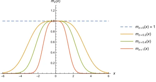
It is worth mentioning thathzcan be interpreted naturally within the framework of position-dependent mass oscillators (see [58, 59, 60, 61, 62, 63, 64, 65] and references therein). The above Hamiltonian naturally suggests the definition of a position-dependent mass function in the form
mz(x) :=
1 shc(zx2) =
zx2
sh(zx2), zlim→0mz(x) = 1, x→±∞lim mz(x) = 0. (4.18)
Then hz can be rewritten as
hz=
Thus the Hamiltonianhz can be regarded as a system corresponding to a particle with position-dependent mass mz(x) under a deformed oscillator potential Uz,osc(x) with time-dependent
-6 -4 -2 0 2 4 6 x 0.2
0.4 0.6 0.8 1.0 1.2 mz(x)
mz=0(x) =1
mz=0.2(x)
mz=0.4(x)
mz=1(x)
Figure 1: The position-dependent mass (4.18) for different values of the deformation parameterz.
-3 -2 -1 0 1 2 3 x
1 2 3 4 5 6 7
Uz,osc(x)
Uz=0,osc(x) =x2
Uz=0.2,osc(x)
Uz=0.4,osc(x)
Uz=1,osc(x)
Figure 2: The deformed oscillator potential (4.19) for different values of the deformation parameterz.
The deformed mass and the oscillator potential functions are represented in figures 1 and 2. The Hamilton equations (4.16) can easily be expressed in terms of mz(x) as
˙
x= ∂h
MP z ∂p =
p mz(x),
˙
p=−∂h MP z
∂x =−mz(x)Ω
2(t)xshc(zx2) + c mz(x)
ch(zx2)
x3shc3(zx2) +p
2 m0z(x)
2m2 z(x)
,
and the constant of the motion (4.17) turns out to be
Fz(2) = 1 4
(x1p2−x2p1)2 mz(x1)mz(x2)
+c mz(x1)mz(x2) shc2 z(x21+x22) (x
2 1+x22)2
x21x22
5
Deformed complex Riccati equation
In this section we consider the complex Riccati equation given by
dz
dt =b1(t) +b2(t)z+b3(t)z
2, z∈
C, (5.1)
wherebi(t) are arbitraryt-dependent real coefficients. We recall that (5.1) is related to certain
planar Riccati equations [49, 50] and that several mathematical and physical applications can be found in [66, 67, 68, 69].
By writing z=u+iv, we find that (5.1) gives rise to a system of the type (2.1), namely
du
dt =b1(t) +b2(t)u+b3(t)(u
2−v2), dv
dt =b2(t)v+ 2b3(t)uv. (5.2)
Thus the associatedt-dependent vector field reads
X=b1(t)X1+b2(t)X2+b3(t)X3, (5.3)
where
X1 = ∂
∂u, X2 =u ∂ ∂u +v
∂
∂v, X3 = (u
2−v2) ∂
∂u+ 2uv ∂
∂v, (5.4)
span a Vessiot–Guldberg Lie algebra VCR 'sl(2) with the same commutation relations (4.5). It has already be proven that the system X is a LH one belonging to the class P2 [22, 23] and
that their vector fields span a regular distribution on R2v6=0. The symplectic form, coming from
(2.4), and the corresponding Hamiltonian functions (2.5) turn out to be
ω= du∧dv
v2 , h1 =−
1
v, h2=− u
v, h3=−
u2+v2
v , (5.5)
which fulfill the commutation rules (4.7) so defining a LH algebra HCR
ω . At-dependent
Hamil-tonian associated withX reads
h=b1(t)h1+b2(t)h2+b3(t)h3. (5.6)
In this case, the constants of the motion (2.18) are found to beF = 1 and [23]
F(2) = (u1−u2)
2+ (v
1+v2)2 v1v2
. (5.7)
As commented above, the Riccati system (5.2) is locally diffeomorphic to the MP equations (4.2) withc >0, both belonging to the same class P2 [22]. Explicitly, the change of variables
x=±c 1/4 p
|v|, y=∓ c1/4u
p
|v|, u=− y
x, |v|= c1/2
x2 , c >0, (5.8)
map, in this order, the vector fields (4.4) onR2x6=0, the symplectic formω= dx∧dy, Hamiltonian
functions (4.6) and the constant of motion (4.10) onto the vector fields (5.4) onR2v6=0, (5.5) and
(5.7) (up to a multiplicative constant ±1 2c
1/2).
Proposition 5.1. (i) The Hamiltonian functions given by
fulfill the commutation rules (4.13) with respect to the Poisson bracket induced by the symplectic formω (5.5) defining the deformed Poisson algebra C∞(HCR∗
z,ω ).
(ii) The corresponding vector fields Xz,i read
Xz,1 =
Next the deformed counterpart of the Riccati Lie system (5.3) and of the LH one (5.6) is defined by
Xz :=b1(t)Xz,1+b2(t)Xz,2+b3(t)Xz,3, hz :=b1(t)hz,1+b2(t)hz,2+b3(t)hz,3. (5.9)
And thet-independent constants of motion turn out to beFz = 1 and
Fz(2)= Therefore the deformation of the system (5.2), defined byXz (5.9), reads
du
6
Deformed coupled Riccati equations
As a last application, let us consider two coupled Riccati equations given by [48]
du
dt =a0(t) +a1(t)u+a2(t)u
2, dv
dt =a0(t) +a1(t)v+a2(t)v
2, (6.1)
constituting a particular case of the systems of Riccati equations studied in [21, 53]. Clearly, the system (6.1) is a Lie system associated with a t-dependent vector field
close on the commutation rules (4.5), so spanning a Vessiot–Guldberg Lie algebraV2R'sl(2). Furthermore, X is a LH system which belongs to the class I4 [22, 23] restricted to R2u6=v. The
symplectic form and Hamiltonian functions for X1,X2,X3 read ω = du∧dv
Hence, thet-dependent Hamiltonian associated with X is given by
h=a0(t)h1+a1(t)h2+a2(t)h3. (6.5)
The constants of the motion (2.18) are nowF =−1/4 and [23]
F(2) =−(u2−v1)(u1−v2)
(u1−v1)(u2−v2)
. (6.6)
The LH system (6.1) is locally diffeomorphic to the MP equations (4.2) but now with
c <0 [22]. Such a diffeomorphism is achieved through the change of variables given by
x=±(4|c|)
Hamiltonian functions (4.6) and constant of motion (4.10) onto (6.3) with domain R2u6=v, (6.4)
and (6.6) (up to a multiplicative constant ±|c|1/2), respectively.
As in the previous section, the (non-standard) deformation of the coupled Riccati system (6.1) is obtained by starting again from proposition 4.1 and now applying the change of variables (6.7) withc=−1 (without loss of generality) finding the following result.
Proposition 6.1. (i) The Hamiltonian functions given by
hz,1 =
satisfy the commutation relations (4.13) with respect to the symplectic form ω (6.4) and define the deformed Poisson algebra C∞(H2R∗
z,ω).
(ii) Their corresponding deformed vector fields turn out to be
The deformed counterpart of the coupled Ricatti Lie system (6.2) and of the LH one (6.5) is defined by
Xz :=a0(t)Xz,1+a1(t)Xz,2+a2(t)Xz,3, hz :=a0(t)hz,1+a1(t)hz,2+a2(t)hz,3. (6.8)
And thet-independent constants of motion areFz =−1/4 and
Fz(2)= e
Therefore, the deformation of the system (6.1) is determined byXz(6.8). Note that the resulting
system presents a strong interaction amongst the variables (u, v) through z, which goes far beyond the initial (naive) coupling corresponding to set the same t-dependent parametersai(t) in both one-dimensional Riccati equations; namely
du
In this work, the notion of Poisson–Hopf deformation of LH systems has been proposed. This framework differs radically from other approaches to the LH systems theory [4, 7, 15, 19, 21], as our resulting deformations do not formally correspond to LH systems, but to an extended notion of them that requires a (non-trivial) Hopf structure and is related with the non-deformed LH system by means of a limiting process in which the deformation parameterzvanishes. Moreover, the introduction of Poisson–Hopf structures allows for the generalization of the type of systems under inspection, since the finite-dimensional Vessiot–Guldberg Lie algebra is replaced by an involutive distribution in the Stefan–Sussman sense.
in that case, the deformation function would be shc(zqp) instead of shc(zq2); this can clearly be seen in the corresponding symplectic realization given in [73]. This fact explains that, in order to illustrate our approach, we have chosen the non-standard deformation of sl(2) due to its physical applications. In spite of this, the Drinfel’d–Jimbo deformation would provide another deformation for the MP and Riccati equations which would be non-equivalent to the ones here studied.
There are still many questions to be analyzed in detail. Since the formalism here presented is applicable in a more wide context, with other types of Hopf algebra deformations and dealing with higher-dimensional Vessiot–Guldberg Lie algebras, this would lead to a richer spectrum of properties for the deformed systems that deserve further investigation. For instance, the deformed LH systems studied in this work are such that the distribution spanned by the deformed vector fields is the same as the initial one. As it has been observed previously, this constraint could not be preserved for generic Poisson–Hopf algebra deformations of LH systems defined on more general manifolds.
An important question to be addressed is whether this approach can provide an effective procedure to derive a deformed analogue of superposition principles for deformed LH systems. Also, it would be interesting to know whether such a description is simultaneously applicable to the various non-equivalent deformations, like an extrapolation of the notion of Lie algebra contraction to Lie systems. Another open problem worthy to be considered is the possibility of getting a unified description of such systems in terms of a certain amount of fixed ‘elementary’ systems, thus implying a first rough systematization of LH-related systems from a more general perspective than that of finite-dimensional Lie algebras. Work in these directions is currently in progress.
Appendix. The hyperbolic sinc function
The hyperbolic counterpart of the well-known sinc function is defined by
shc(x) :=
sh(x)
x , forx6= 0,
1, forx= 0.
The power series around x= 0 reads
shc(x) = ∞
X
n=0 x2n
(2n+ 1)!.
And its derivative is given by
d
dxshc(x) =
ch(x)
x −
sh(x)
x2 =
ch(x)− shc(x)
x .
Hence the behaviour of shc(x) and its derivative remind that of the hyperbolic cosine and sine functions, respectively. We represent them in figure 3.
A novel relationship of the shc function (and also of the sinc one) with Lie systems can be established by considering the following second-order ordinary differential equation
td 2x
dt2 + 2
dx
dt −η
-4 -2 2 4 x
-4
-2 2 4 6
shc(x)
ch(x)
d
dxshc(x) sh(x)
Figure 3: The hyperbolic sinc function versus the hyperbolic cosine function and the derivative of the former versus the hyperbolic sine function.
whereη is a non-zero real parameter. Its general solution can be written as
x(t) =Ashc(ηt) +B ch(ηt)
t , A, B∈R.
Notice that if we setη =iλ withλ∈R∗ we recover the known result for the sinc function:
td 2x
dt2 + 2
dx
dt +λ
2t x= 0, x(t) =Asinc(λt) +B cos(λt)
t . (A.2)
Next the differential equation (A.1) can be written as a system of two first-order differential equations by setting y= dx/dt, namely
dx
dt =y,
dy
dt =−
2
ty+η 2x.
Remarkably enough, these equations determine a Lie system with associatedt-dependent vector field
X=−2
t X1+X2+η 2X
3, (A.3)
where
X1 =y ∂
∂y, X2=y ∂
∂x, X3 =x ∂
∂y, X4 =x ∂ ∂x +y
∂ ∂y,
fulfill the commutation relations
[X1,X2] =X2, [X1,X3] =−X3, [X2,X3] = 2X1−X4, [X4,·] = 0.
Hence, these vector fields span a Vessiot–Guldberg Lie algebraV isomorphic togl(2) with domain
R2x6=0. In fact, V is diffeomorphic to the class I7 'gl(2) of the classification given in [22]. The
diffemorphism can be explictly performed by means of the change of variables u = y/x and
v= 1/x, leading to the vector fields of class I7 with domainR2v6=0 given in [22]
X1 =u ∂
∂u, X2 =−u 2 ∂
∂u −uv ∂
∂v, X3 = ∂
ThereforeX (A.3) is a Lie system but not a LH one since there does not exist any compatible symplectic form satisfying (2.4) for class I7 as shown in [22].
Finally, we point out that the very same result follows by starting from the differential equation (A.2) associated with the sinc function.
Acknowledgments
A.B. and F.J.H. have been partially supported by Ministerio de Econom´ıa y Competitividad (MINECO, Spain) under grants MTM2013-43820-P and MTM2016-79639-P (AEI/FEDER, UE), and by Junta de Castilla y Le´on (Spain) under grants BU278U14 and VA057U16. The research of R.C.S. was partially supported by grant MTM2016-79422-P (AEI/FEDER, EU). E.F.S. acknowledges a fellowship (grant CT45/15-CT46/15) supported by the Universidad Complutense de Madrid. J. de L. acknowledges funding from the Polish National Science Centre under grant HARMONIA 2016/22/M/ST1/00542.
References
[1] Lie S and Scheffers G 1893Vorlesungen ¨uber continuierliche Gruppen mit geometrischen und anderen Anwendungen(Leipzig: Teubner)
[2] Vessiot E 1895 ´Equations diff´erentielles ordinaires du second ordreAnnales Fac. Sci. Toulouse 1`ere S´er.91–26
[3] Davis H T 1962 Introduction to Nonlinear Differential and Integral Equations (New York: Dover Academic Publishers)
[4] Winternitz P 1983 Lie groups and solutions of nonlinear differential equationsNonlinear phenomena (Lectures Notes in Physicsvol 189) ed K B Wolf (New York: Springer) 263–331
[5] Cari˜nena J F, Grabowski J and Marmo G 2000Lie–Scheffers systems: a geometric approach(Naples: Bibliopolis)
[6] Cari˜nena J F, Grabowski J and Marmo G 2007 Superposition rules, Lie theorem and partial differential equationsRep. Math. Phys.60237–258
[7] Cari˜nena J F and de Lucas J 2011 Lie systems: theory, generalisations, and applications, Disserta-tions Math. (Rozprawy Mat.)4791–162
[8] Abe E 1980 Hopf Algebras Cambridge Tracts in Mathematics 74 (Cambridge: Cambridge Univ. Press)
[9] Chari V and Pressley A 1994A Guide to Quantum Groups(Cambridge: Cambridge Univ. Press)
[10] Majid S 1995Foundations of Quantum Group Theory(Cambridge: Cambridge Univ. Press)
[11] Ballesteros A and Ragnisco O 1998 A systematic construction of completely integrable Hamiltonians from coalgebrasJ. Phys. A: Math. Gen.313791–3813
[12] Ballesteros A, Blasco A, Herranz F J, Musso F and Ragnisco O 2009 (Super)integrability from coalgebra symmetry: Formalism and applicationsJ. Phys.: Conf. Ser.175012004
[13] Ballesteros A, Marrero J C and Ravanpak Z 2017 Poisson–Lie groups, bi-Hamiltonian systems and integrable deformationsJ. Phys. A: Math. Theor.50 145204
[14] Ballesteros A, Blasco A and Musso F 2016 Integrable deformations of R¨ossler and Lorenz systems from Poisson–Lie groupsJ. Differential Equations 2608207–8228
[16] Vaisman I 1994Lectures on the geometry of Poisson manifoldsProgress in Mathematics118(Basel: Birkh¨auser Verlag)
[17] Palais R S 1957A global formulation of the Lie theory of transformation groupsMemoirs American Math. Soc. 22(Providence RI: AMS)
[18] Cari˜nena J F, Ibort A, Marmo G and Morandi G 2015 Geometry from Dynamics, Classical and Quantum(Springer: New York)
[19] Carine˜na J F, Grabowski J and de Lucas J 2010 Lie families: theory and applicationsJ. Phys. A: Math. Theor.43305201
[20] Cari˜nena J F, Grabowski J and de Lucas J 2012 Superposition rules for higher-order systems, and their applicationsJ. Phys. A: Math. Theor. 45185202
[21] Ballesteros A, Cari˜nena J F, Herranz F J, de Lucas J and Sard´on C 2013 From constants of motion to superposition rules for Lie–Hamilton systems J. Phys. A: Math. Theor.46285203
[22] Ballesteros A, Blasco A, Herranz F J, de Lucas J and Sard´on C 2015 Lie–Hamilton systems on the plane: Properties, classification and applicationsJ. Differential Equations2582873–2907
[23] Blasco A, Herranz F J, de Lucas J and Sard´on C 2015 Lie–Hamilton systems on the plane: applications and superposition rules J. Phys. A: Math. Theor.48345202
[24] Campoamor-Stursberg R 2016 Low Dimensional Vessiot–Guldberg Lie Algebras of Second-Order Ordinary Differential EquationsSymmetry 88030015
[25] Campoamor-Stursberg R 2016 A functional realization of sl(3,R) providing minimal Vessiot–
Guldberg–Lie algebras of nonlinear second-order ordinary differential equations as proper subal-gebrasJ. Math. Phys.57063508
[26] Ibragimov N H and Gainetdinova A A 2016 Three-dimensional dynamical systems admitting non-linear superposition with three-dimensional Vessiot–Guldberg-Lie algebras Appl. Math. Lett. 52
126–131
[27] Ibragimov N H and Gainetdinova A A 2017 Classification and integration of four-dimensional dynamical systems admitting non-linear superpositionInt. J. Non-linear Mech. 9050–71
[28] Herranz F J, de Lucas J and Tobolski M 2017 Lie–Hamilton systems on curved spaces: A geometrical approach J. Phys. A: Math. Gen.50495201
[29] Ohn Ch 1992 A ∗-product on SL(2) and the corresponding nonstandard quantum-U(sl(2)) Lett. Math. Phys. 2585–88
[30] Ballesteros A, Herranz F J, del Olmo M A and Santander M 1995 Non-standard quantum so(2,2) and beyondJ. Phys. A: Math. Gen.28941–955
[31] Ballesteros A and Herranz F J 1996 A universal R-matrix for non-standard quantum sl(2,R) J.
Phys. A: Math. Gen.29 L311–L316
[32] Shariati A, Aghamohammadi A and Khorrami M 1996 The universal R-matrix for the Jordanian deformation of sl(2), and the contracted forms of so(4)Mod. Phys. Lett. A11 187–197
[33] Gomez X 2000 Classification of three-dimensional Lie bialgebrasJ. Math. Phys.41 4939
[34] Ballesteros A and Musso F 2013 Quantum algebras as quantizations of dual Poisson–Lie groupsJ. Phys. A: Math. Theor.46195203
[35] Ballesteros A, Blasco A, Musso F 2012 Non-coboundary Poisson–Lie structures on the book group
J. Phys. A: Math. Theor. 45105205
[37] Drinfel’d V G 1987 Quantum GroupsProc. Int. Congress of Math.(Berkeley 1986) ed A V Gleason (Providence: AMS) 798–820
[38] Semenov-Tyan-Shanskii MA 1992 Poisson-Lie groups. The quantum duality principle and the twisted quantum double Theor. Math. Phys.931292–1307
[39] Ballesteros A, Blasco A, Musso F 2011 Integrable deformations of Lotka–Volterra systems Phys. Lett. A 3753370–3374
[40] Milne W E 1930 The numerical determination of characteristic numbersPhys. Rev.35863–867
[41] Pinney E 1950 The nonlinear differential equationy00+p(x)y+cy−3 = 0Proc. Amer. Math. Soc. 1681
[42] Ermakov V P 2008 Second-order differential equations: conditions of complete integrabilityAppl. Anal. Discrete Math. 2(2) 123–45 (Translated from the 1880 Russian original by Harin A O and edited by Leach P G L)
[43] Leach P G L 1991 Generalized Ermakov systemsPhys. Letters A158102–106
[44] Leach P G L and Andriopoulos K 2008 The Ermakov equation: a commentaryAppl. Anal. Discrete Math. 2146–157
[45] Fri˘s J, Mandrosov V, Smorodinsky Y A, Uhl´ı˘r M and Winternitz P 1965 On higher symmetries in quantum mechanicsPhys. Lett. 16354–356
[46] Ballesteros A, Herranz F J and Musso F 2013 The anisotropic oscillator on the 2D sphere and the hyperbolic planeNonlinearity26971–990
[47] de Lucas J and Sard´on C 2013 On Lie systems and Kummer–Schwarz equationsJ. Math. Phys.54
033505
[48] Mariton M and Bertrand P 1985 A homotophy algorithm for solving coupled Riccati equations
Optim. Control Appl. Meth. 6351–357
[49] Egorov A I 2007Riccati equationsRussian Academic Monographs5(Sofia-Moscow: Pensoft Publ.)
[50] Wilczy´nski P 2008 Planar nonautonomous polynomial equations: the Riccati equationJ. Differential Equations 2441304–1328
[51] Suazo E, Suslov K S and Vega-Guzm´an J M 2011 The Riccati differential equation and a diffusion-type equationNew York J. Math.17A225–244
[52] Suazo E, Suslov K S and Vega-Guzm´an J M 2014 The Riccati system and a diffusion-type equation
Mathematics2014 96–118
[53] Cari˜nena J F, Grabowski J, de Lucas J and Sard´on C 2014 Dirac–Lie systems and Schwarzian equationsJ. Differential Equations2572303–2340
[54] Est´evez P G, Herranz F J, de Lucas J and Sard´on C 2016 Lie symmetries for Lie systems: Applications to systems of ODEs and PDEs Appl. Math. Comput.273435–452
[55] Ray J R, Reid J L 1979 More exact invariants for the time-dependent harmonic oscillatorPhys. Lett. A71 317–318
[56] Ballesteros A and Herranz F J 2007 Universal integrals for superintegrable systems on N-dimensional spaces of constant curvatureJ. Phys. A: Math. Theor. 40F51–F59
[57] Ballesteros A and Herranz F J 1999 Integrable deformations of oscillator chains from quantum algebras J. Phys. A: Math. Gen.32 8851–8862
[58] Cruz y Cruz S, Negro J and Nieto L 2007 Classical and quantum position-dependent mass harmonic oscillatorsPhys. Lett. A369400–406
[60] Cruz y Cruz S and Rosas-Ortiz O 2009 Position-dependent mass oscillators and coherent states J. Phys. A: Math. Theor.42185205
[61] Ballesteros A, Enciso A, Herranz F J, Ragnisco O and Riglioni D 2011 Quantum mechanics on spaces of nonconstant curvature: the oscillator problem and superintegrabilityAnn. Phys.3262053–2073
[62] Ra˜nada M F 2014 A quantum quasi-harmonic nonlinear oscillator with an isotonic termJ. Math. Phys.55082108
[63] Ghosh D and Roy B 2015 Nonlinear dynamics of classical counterpart of the generalised quantum nonlinear oscillator driven by position-dependent massAnn. Phys.353222–237
[64] Mustafa O 2015 Position-dependent mass Lagrangians: nonlocal transformations, Euler-Lagrange invariance and exact solvabilityJ. Phys. A: Math. Theor. 48225206
[65] Quesne Ch 2015 Generalised nonlinear oscillators with quasi-harmonic behaviour: Classical solutions
J. Math. Phys.56 012903
[66] Campos J 1997 M¨obius transformations and periodic solutions of complex Riccati equations Bull. London Math. Soc.29205–215
[67] Farooq M U, Mahomed F M and Rashid M A 2010 Integration of systems of ODEs via nonlocal symmetry-like operators Math. Comput. Appl. 15585–600
[68] Ortega R 2012 The complex periodic problem for a Riccati equationAnn. Univ. Buchar. Math. Ser. 3219–226
[69] Schuch D 2012 Complex Riccati equations as a link between different approaches for the description of dissipative and irreversible systems J. Phys.: Conf. Ser.380012009
[70] von Roos O 1983 Position-dependent effective masses in semiconductor theoryPhys. Rev. B.27 7547
[71] Bastard G 1988Wave mechanics applied to semiconductor heterostructures(Paris: Les ´Editions de Physique)
[72] Harrison P 2009Quantum wells, wires and dots(New York: Wiley)