Journal of Computational Design and Engineering 3 (2016) 337–348
Data-mining modeling for the prediction of wear on forming-taps in the
threading of steel components
Andres Bustillo
a,n, Luis N. López de Lacalle
b, Asier Fernández-Valdivielso
b, Pedro Santos
a aDepartment of Civil Engineering, University of Burgos, Burgos, Spain
b
Department of Mechanical Engineering, University of the Basque Country UPV/EHU, Bilbao, Spain
Received 4 March 2016; received in revised form 16 June 2016; accepted 26 June 2016 Available online 30 June 2016
Abstract
An experimental approach is presented for the measurement of wear that is common in the threading of cold-forged steel. In this work, thefirst objective is to measure wear on various types of roll taps manufactured to tapping holes in microalloyed HR45 steel. Different geometries and levels of wear are tested and measured. Taking their geometry as the critical factor, the types of forming tap with the least wear and the best performance are identified. Abrasive wear was observed on the forming lobes. A higher number of lobes in the chamber zone and around the nominal diameter meant a more uniform load distribution and a more gradual forming process. A second objective is to identify the most accurate data-mining technique for the prediction of form-tap wear. Different data-mining techniques are tested to select the most accurate one: from standard versions such as Multilayer Perceptrons, Support Vector Machines and Regression Trees to the most recent ones such as Rotation Forest ensembles and Iterated Bagging ensembles. The best results were obtained with ensembles of Rotation Forest with unpruned Regression Trees as base regressors that reduced the RMS error of the best-tested baseline technique for the lower length output by 33%, and Additive Regression with unpruned M5P as base regressors that reduced the RMS errors of the linearfit for the upper and total lengths by 25% and 39%, respectively. However, the lower length was statistically more difficult to model in Additive Regression than in Rotation Forest. Rotation Forest with unpruned Regression Trees as base regressors therefore appeared to be the most suitable regressor for the modeling of this industrial problem.
&2016 Society of CAD/CAM Engineers. Publishing Servies by Elsevier. This is an open access article under the CC BY-NC-ND license (http://creativecommons.org/licenses/by-nc-nd/4.0/).
Keywords:Roll-tap wear; Roll taps; Threading; Forming taps; Ensembles; Rotation forest; Regression trees
1. Introduction
There are two basic technologies for manufacturing internal threads: form tapping (using roll/form taps) and cut tapping (using cut taps). Thefirst process is chipless because the thread is formed by a cold-working process. Hence, stronger threads, particularly in materials susceptible to strain hardening, good thread calibration and a longer tool life are achieved. Form tapping is studied in the present work, applied in this case to a forged piece, in which the holes were punched in a cold-forging process. In the case of form tapping, the thread is formed by deformation of the raw material in a cold-working process[1].
This process causes an imperfection at a minor diameter of the formed threads (thread peaks) referred to as a claw or a split crest, although these imperfections imply no reduction in strength[2,3]. Claw shapes depend on the hole diameter before threading [4]. Form tapping can be performed on ductile steels, non-ferrous alloys[5]and tempered steels[6].
Stéphan et al.[7]maintained an acceptable forming torque and deep enough threads to avoid stripping problems by optimization of the initial hole diameter. Fromentin et al.[8]studied the 3D plastic flow in form tapping, measuring material displacement and Stéphan et al. [9] developed a 3D finite element model for form tapping with the ABAQUS 6.5 software program.
The prediction of tap wear involves three degradation phenomena: adhesive, abrasive and erosive wear. Adhesive wear is caused by the transfer of material from one surface to the other. Abrasive wear is caused by material removal from a www.elsevier.com/locate/jcde
http://dx.doi.org/10.1016/j.jcde.2016.06.002
2288-4300/&2016 Society of CAD/CAM Engineers. Publishing Servies by Elsevier. This is an open access article under the CC BY-NC-ND license (http://creativecommons.org/licenses/by-nc-nd/4.0/).
nCorresponding author. Fax:þ34 947258910.
E-mail address:abustillo@ubu.es(A. Bustillo).
solid surface, due to the sliding effect of hard particles or roughness peaks against the other contact surface. Finally, erosive wear is material loss from a solid surface, due to the action of a fluid containing solid particles.
Simulations were focused on external thread manufacturing by deformation [10]. Domblesky [11]worked on the simulation of thread rolling with good accuracy and then on the optimization of process parameters [12]. The most direct approach involves a macroscopic description of worn surfaces and empirical modeling of the wear based on the process parameters[13].
Data-mining represents a collection of computational tech-niques, which analyze very complex phenomena. The most common data-mining techniques applied to manufacturing problems include Artificial Neural Networks (ANNs), Support Vector Machines (SVMs), k-Nearest Neighbors Regressors, and Regression Trees. A combination of two or more models, known as an ensemble, sums the predictions capabilities of the combined models. Ensembles have demonstrated their super-iority over single models in many applications. For instance, Yü [14] used ensembles to identify out-of-control signals in multivariate processes. Liao et al.[15]and Bustillo and Rodriguez [16] used ensembles for grinding wheel and multitooth tool condition monitoring, respectively, while Cho [17] and Bisaeid [18]used ensembles for end-milling condi-tion monitoring and simultaneous deteccondi-tion of transient and gradual abnormalities in end milling. Ensembles have the advantage of circumventing the fine tuning of other artificial intelligence models such as ANNs [19]. The most common types of ensemble techniques are Bagging, Boosting and Random Subspaces. Finally, a recent ensemble technique, Rotation Forest [20], has demonstrated a capability to model different industrial problems[21]. All these techniques will be presented in detail in Section 3. To the best of the authors' knowledge, there are no other investigations that have modeled form tapping process outputs with data-mining techniques. One novel robust approach for root-cause identification in machining process using a hybrid learning algorithm and engineering-driven rules was developed by Shichang et al. [22]. In contrast, Mazahery[23]proposed the use of ANN for tribological behavior modeling of composites, adjusting the weights and biases in the network during the training stage to minimize modeling error. In relation to aluminum
nanocomposite processing, Mazahery [24] proposed the use of genetic algorithms to predict the mechanical properties and to optimize the process conditions and Shabani [25] used adaptive neuro-fuzzy inference systems combined with the particle swarm optimization method for process optimization. The novelty of this paper resides in its combination of an experimental analysis and a data-mining model to extract as much information as possible on tool wear in form tapping processes, an industrial process in high demand. The Multi-layer Perceptron, the most widely used standard artificial intelligence technique mentioned in the literature, was used to identify the baseline improvements of this new approach [19]. This paper is structured as follows: at the end of this introduction, Section 2 presents the fundamentals of form tapping and the experimental set-up realized to obtain real data for this industrial process;Section 3introduces the data-mining techniques that will be used to model these industrial data; Section 4presents and discusses the experimental results of the measurements and of the modeling using the data-mining techniques; finally, Section 5 sums up the main conclusions obtained from this research and future lines of work.
2. Form tapping fundamentals and experimental procedure
2.1. Form tapping
Tap geometry is the most important parameter for a reliable process. The standard tap characteristics are chamfer length, the number of pitches in the chamfer, tap diameter and the number of lobes around a tap section. Fig. 1 shows the geometry and features of a typical forming tap. All pictures showing taps are oriented with the tap tip to the left. As shown inFig. 1, each rounded corner of a tap section is referred to as a lobe, where deformation or friction occurs against the inner surface of the previous hole. Hence, the tap section is defined by a curved side polygon that may typically have three,five, or six corners, which are referred to as lobes.
Three type of lobes are distinguished in each tap: i) incremental forming lobes situated in the chamfer area; ii) calibration forming lobes around the nominal diameter; and, finally, iii) guiding lobes leading up to the tap shank. The
shapes of the calibration and the guiding lobes are not so very different, so the precise frontier between them is a function of tap wear and is not exact, as will be shown later on. With regard to the application of data-mining techniques, the variation in length on the rake side (upper length) and in the length on the relief side has been considered (down length) for each lobe, as well as the variation in the total length of each lobe.
Two types of wear are observed in forming taps: material abrasive wear and adhesive wear. Abrasive wear is mainly observed in the lobes that remain in contact with the material during the material removal process. If they are in the chamfer region of the forming tap, the lobes are increasingly concave and spread out on the side at variable depths that are as deep as the part of the thread in contact with the tool. In the case of a lobe located on the guiding zone, with the nominal diameter, contact with the material is up until the moment of elastic recovery, and the height of the areas on the flanks is at a maximum, since the thread is totally formed during the moment of contact.
Adhesive wear is defined as follows. Coating wear always begins at the front of the lobe. Initially, delamination is likely and then, as the wear becomes more progressive, it will probably be associated with abrasive friction. Steel may be deposited on the frontal part of the lobe, by adhesion on the area of the coating with abrasive wear. The material is deposited on the front side of the lobe and it extends to cover the lobe in the opposite direction to the abrasive wear of the back lobe. The adhesion is therefore described asrunout.
2.2. Experimental set-up
The experimental objective was to test different type of roll taps with different geometries and levels of wear. The tapping conditions included external lubrication of 15% emulsion at a pressure of 6 bars, applying the following process parameters: M101.5 form tap ISO dimensions, 1200 mm/min feed speed, 1.5 mm/rev feed rate, 800 rpm rotation speed, and 30 m/min forming speed.
The taps shared the following characteristics: a) base material, high speed steel with TiN coating, and b) 6GX tolerance. Six taps were tested for 3 different types of roll taps (total 18 forming taps). Type 1 had a 5-pitch chamfer with a hexagonal (601) geometry without oil grooves. Type 2 had a
3-pitch chamfer with a pentagonal (721) geometry with oil grooves. Type 3 had a 3-pitch chamfer with a pentagonal (721) geometry without oil grooves. The number of pitches was directly proportional to the length of the chamfer. A high number of pitches in the chamfer area causes problems in blind holes that have requirements for low clearance at the bottom of the hole. Each tap presented different levels of wear, due to previous working in a real workshop, reaching 1000, 2000, 3000, 4000 and 5000 threads, to be compared with a new unworn tap (Fig. 2). Wear analysis and experimental results are exhaustively presented in [13], basically using a field microscope and a special jig for setting tool in the same coordinate measurement system, as it is a common practice in this kind of experimentations.
The thread length of a forming tap is usually manufactured with a higher tolerance than the cut tap equivalent in metric and diameter, due to the degree of elasticity of the material that means the work piece will always contract after any plastic forming process. Consequently, the fresh thread is always slightly smaller than the form tap profile. The operation has to be executed in one stroke, because it is almost impossible to manually repeat the form-tapping process after the first lamination, due to the strain hardening that is provoked by the first operation, which is not a problem in the case of cut taps. Therefore, it is necessary to manufacture the roll taps so that their upper tolerance limit is closest to the internal thread. For this reason, all the taps in the study were 6GX tolerance, to ensure that tolerance was not a factor that could affect the results.
The work piece material was a microalloyed HR45 steel, categorized under the group of microalloyed (HSLA – High Strength Low Alloy) steels. HSLA steel has a fine ferrite-pearlite structure with a small addition (max 0.15%) of the combination of Al, Ti, Nb, and V elements. According to data provided by an end-user, it has the following characteristics: yield strength syp¼359 MPa, ultimate tensile strength su ¼ 473 MPa and final strainA¼34.3%. The small test parts were cold forged and a punch was used to open two holes with a diameter of 9.3 mm and a hardness of 223 HV, measured inside the holes. Cold forging always induces strain hardening, so this measurement is important for a correct interpretation of the results that are presented later on. The test part was a strut that attaches a motor to a vehicle chassis; cold forging ensures a highly productive process.
NEW TAP 3000 THREADS 5000 THREADS
The tests were performed on a 3-axis CNC machine with a 14 kW spindle. All the tests were performed under both dry and lubricated conditions, so as to compare the different taps, forming two threads under each of the two conditions. The objective of using coolant was to avoid overheating in the thread/tap contact area, to increase lubrication, and to study tool behavior under industrial conditions. Otherwise, the dry condition was used because monitoring was more directly related to tap damage state.
Thus, tap wear measurements were taken on all the lobes in the chamfer zone to establish a baseline wear value for the graph: on the lobes that were slightly smaller than the nominal diameter and on successively wider ones. When the nominal diameter lobes started to lose their geometry, the successive ones continued to work and they also registered wear. It should be remembered that the forming lobes induce strain hardening and therefore the last lobe in the chamfer zone deforms the work piece material in its hardest state. Deformation not completed by this lobe must be completed by the successive ones.
In short, the procedure consisted of measuring wear after form tapping, under two different conditions, dry and with drilling fluid, with new taps and with taps after 1000, 2000, 3000, 4000 and 5000 previous threads formed under real working conditions in a company that used the same type of toolholder and emulsion coolant.
2.3. Dataset generation
Having measured tap wear in each experiment, 3 datasets for the data-mining models were generated: one for each output. Among the variables that influenced the wear process, the following were considered: type of forming taps, number of threads and lobe of the tap. Lobes are numbered starting from the first one at the tap tip, as previously explained. Tap wear was evaluated in terms of the variation from nominal values of 3 lengths for each lobe of the tap: lower length, upper length (always starting from the maximum outer diameter of the forming lobe) and total length, as previously presented (see Fig. 1in Section 2).Table 1 summarizes the variables under consideration and their variation range and whether they act as input or output for the data-mining model. Although most of these variables take a limited number of values due to the definition of the experiment, the data-mining model will consider the number of threads and the 3 outputs as continuous variables, because they can take continuous values under industrial conditions. Other variables, such as the type of forming tap and tap lobe, are considered categorical variables: the type of forming tap only takes 3 possible values and the lobe of the tap takes 25, seeTable 1. Only the 25first lobes are considered in the data-mining models, because they are the only ones common to the three forming taps, even though the 3 types of roll tapshave a different number of lobes.
As previously explained, the smaller diameter tap lobes showed no wear until the chamfer diameter was sufficiently wide to engage the material. The data set therefore contains many zeros that reflect no-wear in the lobes. From the 435
instances of each of the 3 data sets, 109, 123 and 131 instances recorded a zero value for the output, seeTable 1. These zero values mean that around 30% of the experiments show no-wear on the measured lobe of the tap. If a data-mining technique evaluates this data set it will be programmed to prioritize zero values to increase its accuracy.
3. Data-mining techniques
As explained in the introduction, the data-mining discipline provides algorithms to forecast the values of some output variables from a set of input variables. There are two types of prediction techniques: regression, if the studied variable can take continuous values, andclassification, when the output can only vary between a limited set of values. In our experimental work, a regression analysis is formed for each output variable, y. In this type of formulation, the forecast of the model is based on a function,f, of the so-calledattributes(input variables),x. This general expression for regression is shown in Eq. (1), considering a case withmattributes.
yestimated¼f xð Þ; xAℜm; yAℜ ð1Þ
The most precise technique for the problem under study was chosen from the algorithms of the state-of-the-art for regres-sion. Root Mean Squared Error (RMSE) was used to compare the regressors This metric measures the deviation that the predicted class value has with regard to its real value. The expression of RMSE is given by the square root of the mean of the squares of the deviations, as Eq.(2)shows, where each of then instances of the data set are denoted byxi;yi.
The most popular regression techniques were used in the tests. These algorithms can be divided into four families:
1. Decision tree regressors: the consideration of this type of techniques is necessary to understand the second family: the ensemble regressors.
2. Ensemble techniques [26]: the most frequently used algo-rithms were tested, as they have proved their suitability in several types of industrial tasks [14–19,21,27].
Table 1
Variables, units and ranges used to generate the dataset.
Variable [Units] Input/
output
Range [number of zeros]
Type of forming taps Input 1, 2, 3 (Type 1, 2 and 3)
Lobe of the tap Input 1–25
Number of threads Input 1,000–5,000
Upper length [mm] (on
3. Function-based regressors: ANNs[28]and Support Vector Regression (SVR)[29]were used. The choice of SVR and ANNs was due to their popularity The success of ANNs in modeling several industrial problems should be noted [30–33], while SVR is a widely used regression technique [34].
4. The approach of instance-based regressors has a completely different formulation from the other families, as there is no analytic model to express the class value as a function of the attributes. Alternatively, the forecast value is obtained by the instance similarity to some other instances in the training dataset. The k-Nearest Neighbors Regressor [35] was used in the tests as representative of this type of prediction.
3.1. Decision-tree-based regressors
Following a strategy known as divide and conquer, a decision-tree-based regressor uses recursive data divisions in a single attribute. Each division is performed by maximizing the differences observed between the class values [36], while several statistical procedures may be used to determine the most discriminant decision.
There are two types of regressors based on decision trees, depending on what they store in their leaves. While a linear regression model is saved in each leaf of the model trees, an average of the values of a group of instances is used in the regression trees, minimizing the intrasubset variation in the class values [37]. The Reduced-Error Pruning Tree (REPTree) [38] and M5P [36] were chosen as the main representative techniques for the regression and the model trees, respectively.
Both regressors have two possible configurations: pruned and unpruned trees. Considering a single tree-based regressor and some type of ensembles of regression trees, it is more convenient to use pruned trees to avoid overtfitting. However, there are certain types of regression tree ensembles that can benefit from the use of unpruned trees [39]. Ensembles of regression trees are described in the next section.
3.2. Ensemble regressors
An ensemble regressor is a prediction method that combines the forecasts of several models: the base regressors [40]. In this work, the three most popular types of ensembles were used: Bagging [41], Boosting [42] and Random Subspaces [39]. In these three regression techniques, the same learning algorithm is used to train each base regressor, but different training sets are formed from the original. In all cases, we used regression trees as base regressors.
In Bagging, the training sets were formed using sampling with replacements (i.e., given a training set, a particular instance may not appear in it or could appear several times) [41]. The base regressors were independent, as the process followed to train each base regressor takes no account of the other regressor. One variant of Bagging is called IteratedBag-ging. This technique combines Bagging ensembles: the first
one is formed by conventional Bagging, but the differences between the real and the predicted values (calledresiduals) are used in the training process for the others [43].
On the contrary, the base regressors in the case of Boosting, are sequentially trained, each one of which is influenced by the previous one[44]. A weight is added to the instances, in order to change the training of the base regressors. The errors of previous regressors are used to reweight the instances, so that the next regressor is trained with the instances that were previously wrongly forecast. The final prediction of Boosting also takes the accuracy of each base regressor into account. One common variation of Boosting implementation for regres-sion is AdaBoost.R2[45]. In this case, the error of each base regressor is calculated using theloss function,L(i). Three types of loss functions were used in the experimentation. If Denis the maximum value of a loss function, then linear loss, Ll, square loss, Ls and exponential loss, Le, are given by the expressions in Eq. (3).
Llð Þ ¼i l ið Þ=Den
Random Subspaces uses subsets of fewer dimensions than the original data set to train the base regressors. This methodology has two goals. On the one hand, to avoid the well-known problem of the curse of dimensionality (many regressors decrease their performance when the data sets have a large number of attributes), and, on the other, to improve prediction accuracy, by choosing low correlated base regressors.
Rotation Forest [20] is the most recent ensemble tested in this research. It trains each base regressor, in this case RepTrees or M5P Modal Trees, by grouping their attributes into subsets (e.g., subsets of three attributes are usually taken). Then Principal Component Analysis is computed for each group using a subsample from the training set. The whole dataset is transformed according to these projections and can then be used to train a base regressor.
Five ensemble regressors were used in the experimentation: Bagging, IteratedBagging, Random Subspaces and Additive Regression, a hybrid between Bagging and Boosting ensem-bles[46]and Rotation Forest.
3.3. Artificial neural networks
respectively, B1 and B2 their biases, and fnet and foutput their
These activation functions vary with the structure. In our experimental work, the most common structure was used, where the activation function for the hidden layer is the identity and the activation function for the output layer is tansig [49].
3.4. Support vector regressor
This technique makes its prediction using a function, f(x), with a set of parameters that are calculated during the training stage, in order to minimize the RMSE[50]. The formulation of this function for a linear case is given by Eq. (5). The prediction, f(x), from the input attributes, x, is obtained by using terms,wand b, where〈w,x〉is the inner product in the input space, X.
fðxÞ ¼〈w;x〉þb with wAX bAℜ ð5Þ
The desired function should fit the training examples as closely as possible, but without overfitting the data, in order to define a formulation that may be generalized to other instances. In other words, the desired function shows low prediction deviations, but as flat as possible [50]. Expressing these two objectives in an optimization problem, the target is for f(x) to have at mostεdeviation from the forecast outputs, yi, for all the training data, and at the same time to minimize the norms ofw. A certain degree of error will therefore be allowed in the forecasts, but it is limited by ε. In real data, solving the previously described optimization problem may be unfeasible or lead to overfitting, if there are some instances with large deviations of the general trend. For that reason, Boser et al. [29] redefined the optimization problem, allowing deviations larger thanεfor some instances. Consequently, an extra term, C, was added to the formula, as shown in Eq. (6). This parameter is a trade-off between theflatness and the deviations of the errors larger than ε.
minimize 1
The optimization problem presented in Eq. (6) belongs to the convex type, and can be solved using the Lagrange method. Eq. (7) shows the so-called dual problem that is
associated with it.
The formulation given in Eq. (7) refers only to the linear case, but a generalization using a non-linear function is possible. In the general definition of the SVR, the inner products are not directly calculated in the original input feature space, but the so-calledkernel function,k(x,x0) is used instead. This function fulfils a set of conditions (called Mercer's conditions) [51]. Linear and radial basis, the two most frequently referenced kernels in the literature, were used in the experimentation.
3.5. K-nearest neighbor regressor
In this data-mining technique, the predicted class value is the mean of thekmost similar training instances, which were previously stored [52]. Euclidean distance was the most commonly used function to measure the similarity between instances. In our experimental work, the number of neighbors was optimized using cross validation.
4. Results and discussion
4.1. Experimental results
In this section, the results of the experiments on wear measurements are present. First, a visual inspection was undertaken to determine whether the taps had suffered any damage such as lobe ruptures or excessive material adhesion. The lower length and the upper length each lobe edge were measured, commencing in each case with the maximum outer diameter of the forming lobe, as shown inFig. 3. A magnified worn area of a lobe is shown on the right ofFig. 3, measured with an optical microscope. All measurements were taken by positioning taps on the samefixture, so as to avoid projection errors and to ensure sufficient repeatability. In thisfigure, the edge that engages the material is therake edge, while the other length of the edge is therelief edge(both standard industrial terms in cutting operations).
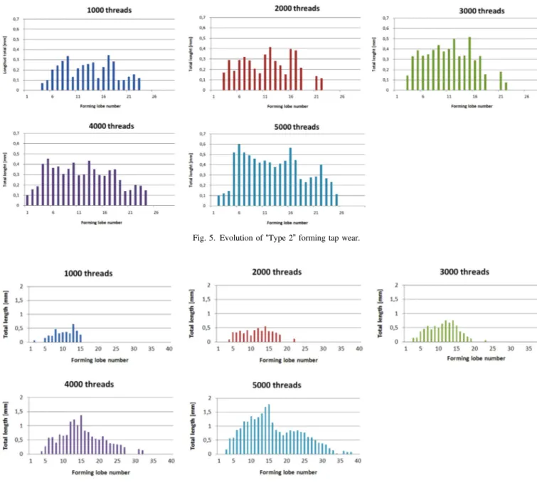
The wear on each lobe is illustrated in Figs. 4–6. Here, the lobes are numbered starting from thefirst one at tap tip. One hypothesis would suggest that worsening wear on each lobe depends on the general wear of the roll tap, because wear on previous lobes would imply a greater strain on the successive ones, as is clearly explained below. All the wear patterns corresponded to abrasion on the rake flank and abrasion and slight adhesion on the reliefflank. The limits of the chamfering zone are indicated on thefigures.
“Type 1” roll taps with previous wear of 1000, 3000 and 4000 threads showed a rising trend line from non-existent wear on thefirst lobes to levels of about 0.1 mm. Furthermore, the higher the number of threads, the higher the tap wear will be. Wear was almost zero for thefirst 4 lobes of an almost new tap with“only”1000 previous threads. It then increased to reach a constant value after the 10th lobe. A provisional conclusion was therefore reached that the first lobe of nominal diameter will not be the most highly damaged.
However, the trend lines of tap wear with 2000 and 5000 threads had a non-linear evolution. The wear was not uniform
in close lobes. The lobes with greater wear interacted more with the material, while the lobes with less wear may have been working less due to the eccentricity of the tap, which could be the explanation for this random behavior.
Contrary to the previous case, the results for “Type 2”roll taps (Fig. 5) pointed to strong wear for the first lobes and a rapid decrease for the following ones to a constant value between the 7th and 16th lobe (Fig. 5). As shown in Fig. 5, wear decreased to zero for the 5 cases (taps with 1000 to 5000 previous threads), it was higher for the last level (5000 threads), and was lower for the first level (1000 threads). Wear evolution was completely different to that of the“type 1” taps. A difference explained by the increased diameter between the pitches in the chamfer zone that was greater than the increase of subsequent threads; the first lobe that reached the nominal diameter worked very intensely.
For “Type 3”roll taps (Fig. 6), the evolution of wear started from zero for the twofirst lobes, increased to a maximum and decreased again. As shown inFig. 6, wear increased as the tap diameter increased. Once the final thread diameter had been
Fig. 3. Forming lobe wear: Left) tap rotation; Right) Wear on the relief (lower) and rake (upper)flanks.
reached, wear on the subsequent lobes decreased, due to lower contact with the material as the thread had recently been formed. The lobes engaging with the material underwent lighter deformation that resulted in less wear (15th to 25th lobe).
The different tap wear behaviors can be attributed to the geometry of the chamfer tap (5-pitch chamfer for “Type 1” forming taps, 3-pitch chamfer for “Type 3” and “Type 2” forming taps) and the number of lobes in each section (hexagonal in“Type 1”, and pentagonal in “Types”2 and 3”). The geometry of“Type 1”led to a more progressive deforma-tion of the material and therefore implied less wear.
In the three roll taps under study, higher wear appeared in the chamfer lobes. When form tapping was at the nominal diameter, the guiding edges were in contact with previously deformed material. For this reason, wear decreased gradually at these edges until it reached zero wear values. Ten guiding lobes in the three roll taps were necessary to reach zero wear level.
4.2. Data-mining prediction results
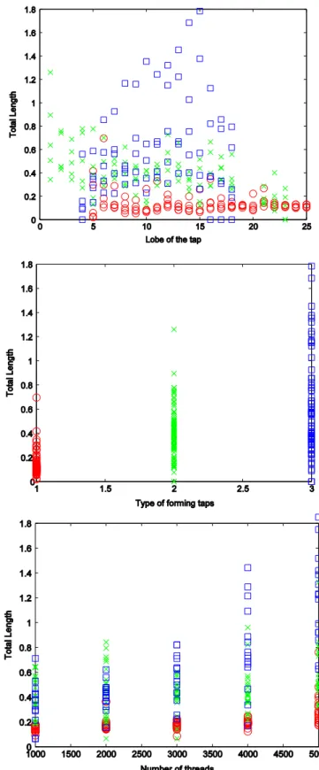
Tap forming is a complex process, in which a direct relationship between process inputs and the output (tap wear) is not easily established. This conclusion has been outlined in the previous analysis of the experimental tests and may also be extracted from a data-mining perspective, if the scatter plots of inputs and outputs are drawn.Fig. 7presents the scatter plots for each input (type of forming taps, lobe of the tap and number of threads) and one of the outputs (total length). These plots show that there is no obvious relation between the input variables and the output. Each symbol, blue square, red circle and yellow cross, represents a different type of forming tap (1 to 3 types respectively). The same conclusion can be extracted for the other two outputs: lower length and upper length. A suitable method is therefore needed to model the tap wear form from the process input variables.
Fig. 5. Evolution of“Type 2”forming tap wear.
However, before the most suitable model for tap wear can be identified, it is necessary to establish a baseline or threshold that assures the right performance of the data-mining models or rejects their predictions due to low quality. The Root Mean Square Error (RMSE) for the predicted values related to the measured values was taken as a quality indicator. Two baseline
approaches were considered: thefirst one is a naive approach, which considers the mean value of each output as the most probable value for each condition; the second one considers a linear fit of the 3 inputs for each output. Table 2 shows the mean, maximum and minimum values of each of the 3 outputs in the dataset and the RMSE values calculated for the naive approach and the linear approach of each output for the whole dataset. From the industrial point of view, any prediction model that reduces the RMSE by more than 20% will provide useful information to the process engineer on tap wear.
As explained inSection 3, the main techniques of the state of art for regression were tested, including regression trees (RepTrees and M5P trees), ensembles (Bagging, Iterated Bagging, Random Subspaces, Adaboost, Additive Regression and Rotation Forest), SVRs, ANNs (MLPs), and nearest neighbor regression. Table 3 summarizes the abbreviations used to denote these techniques. As regards notation, two further considerations should be taken into account. Firstly, in the case Adaboost.R2, the type of loss function is indicated by the suffixes "L", "S" and "E" (Linear, Square and Exponential, respectively). Secondly, whether the trees are pruned or unpruned is indicated between brackets (P or U).
A 1010-fold cross-validation procedure [17] was fol-lowed, to generalize the results of the data mining techniques. In 10-fold cross-validation, the data is divided into 10 folds. Nine folds are used to build a model and the other fold is used to evaluate the model. The estimation obtained with cross-validation is the average of 10 values obtained for each fold. Cross-validation was repeated 10 times, that is 1010-fold
Fig. 7. Scatter plots for each predictive variable and the total length.
Table 2
Dataset variation of the outputs and RMSE for the 2 proposed baselines techniques.
Lower length [mm]
Upper length [mm]
Total length [mm]
Mean value 0.12 0.15 0.27
Maximum 0.77 1.17 1.78
Minimum 0 0 0
RMSE Naïve approach
0.14 0.20 0.30
RMSE Linear approach
0.12 0.16 0.23
Table 3 Methods notation.
Method Abbreviation
Bagging BG
Iterated Bagging IB
Random Subspaces RS
AdaboostR2 R2
Additive Regression AR
Rotation Forest RF
REPTree RP
M5P Model Tree M5P
Support Vector Regressor SVR
Multi-Layer Perceptron MLP
cross validation, averaging the results obtained from each cross-validation, in order to reduce the variance of the final estimation. In this way the prediction of the model is the average of the predictions of 100 models. Weka software[38] was used for modeling and validation.
The parameters of the techniques were chosen as follows:
1. The number of base regressors in the ensembles was set to 100
2. In the SVR with linear Kernel, the trade-off parameter was optimized in the range of 2 to 8, while in the radial basis case, the optimization ranges were 1 to 16 for C and 105 to 102forγ
3. The training parameters momentum, learning rate and number of neurons of the neural networks were optimized in the ranges 0.1 to 0.4, 0.1 to 0.6, 5 to 15, respectively 4. In the k-nearest neighbor regressor, the optimal number of
neighbors was chosen from 1 to 11.
InTable 4the detailed RMSE values are shown for the three outputs under study, where an asterisk indicates the regressors that were statistically worse than the best one for each output (the reference for the test for each output is the regressor with lower RMSE, which is in bold). Table 2 also collects the RMSE for two approaches considered as baselines for afinal discussion of the results. Two main considerations can be extracted from the results ofTable 4:
1. Two methods present the lower RMSE for the three outputs: Rotation Forest with unpruned REPTree as base regressors for the lower length, and Additive Regression with unpruned M5P as base regressors for the upper and total lengths. However, the second method is statistically worse than thefirst one to model the lower length. 2. There are only two methods which do not lose in any of the
three outputs: Rotation Forest with unpruned REPTree as base regressors (the winner for the lower length) and Iterated Bagging with unpruned M5P as base regressors.
Finally, if we compare the results of these prediction models inTable 4 with the two approaches considered as baselines, new conclusions may be extracted. First, all the data-mining techniques under consideration showed a better performance than the naïve approach (e.g. for the lower length the RMSE of the tested techniques was in the range of 0.09–0.12 mm and was 0.14 mm for the naïve approach). Second, not all of the data-mining Techniques under consideration showed a better performance than the linear fit (e.g. the RMSE of the tested techniques for the upper length were within the range 0.12– 0.18 mm and the linear fit was 0.16 mm), There are two reasons that can explain this result:first, the reduction of the dataset size due to the cross-validation technique does not apply to the linearfit, which is significant due to the small size of the dataset; second, training and validation are done on the same data in the linear fit case, while the cross validation technique applied to data-mining models used new data for validation that was not presented in the training step. The most important conclusion, however, even though data mining undergoes a loss of accuracy due to cross validation (because only part of the experimental dataset is used for the training stage, keeping part of the instances for the validation stage), is that there are still some data-mining models that clearly improve the precision of the two baseline techniques (that use the whole experimental dataset in the training stage). For example Rotation Forest with unpruned REPTree as base regressors reduced the RMSE of the linearfit by 33% for the
Table 4
RMSE values for all the tested data-mining techniques.
Method Lower length
Naïve approach 0.14 0.20 0.30 Linear approach 0.12 0.16 0.23 SVR Linear 0.09* 0.17* 0.22* SVR Radial 0.09 0.13 * 0.16 R2 L M5P (P) 0.10* 0.13* 0.15
RF REPTree (U) 0.08 0.13 0.16
lower length, and Additive Regression with unpruned M5P as base regressors reduced the RMSE of the linearfit by 25% and 39%, for the upper and total lengths respectively. Taking all these considerations into account, Rotation Forest with unpruned REPTree as its base regressors appeared to be the most suitable regressor with which to model this industrial problem.
To summarize, the most accurate Data Mining technique is Rotation Forest with unpruned REPTree as base regressors. It predicts the lower, upper and total wear length with an RMSE of 0.08, 0.13 and 0.16 mm respectively. Under similar training conditions, the Naïve approach predictions presents an RMSE of 0.14, 0.20 and 0.30 mm for the same outputs and the linear approach an RMSE of 0.12, 0.16 and 0.23 mm, clearly higher than the RMSE of the Rotation Forest in all cases.
5. Conclusions
This paper has presented a study that has analyzed the process of wear during tap forming for threading of cold forged steel parts from an experimental and a data-mining perspective. Wear observed on the forming lobes was of the abrasive type. This type of wear implies the loss of lobe diameter involving successive lobes. The“Type 1”forming tap had the least wear and showed the best performance. Forming tap geometry appeared to be a very important factor. The “Type 1”hexagonal section tap produced superior results to the “Type 2”and the“Type 3”pentagonal section tap. The higher the number of lobes in the chamber zone (5-pitches) and around the nominal diameter (6 lobes) resulted in a more uniform load distribution and a more gradual forming process. The second objective of this study was to identify the most accurate data-mining-based model to solve this real-life industrial problem. The data set consisted of 285 instances with 3 inputs and 3 outputs. Several methods were investi-gated, including all the main techniques of the state of art for regression: regression trees, ensembles, SVRs, ANNs and k nearest-neighbor regression. 1010 cross-fold validations were performed to generalize the prediction results of these models.
Two baseline approaches were considered to analyze the performance of the data-mining models: the first considered the mean value of each output as the most probable value for each condition; the second considered a linearfit of the 3 inputs for each output. The most accurate model was Rotation Forest with unpruned REPTree as its base regressors; it reduced the RMSE of the linear fit by 33% for the lower length, and the Additive Regression with unpruned M5P as base regressors that reduced the RMSE of the linearfit for the upper and total lengths by 25% and 39% respectively. However, Additive Regression was statistically worse than Rotation Forest at modeling the lower length, and therefore, Rotation Forest with unpruned REPTree as its base regressors appeared to be the most suitable regressor for the modeling of this industrial problem.
Future work will consider other ensemble methods, using ensembles of other methods instead of regression trees and will
study the use of non-homogeneous ensemble models, ensem-bles built by combining different methods (e.g., SVM and RBF), that might improve the final accuracy of the model.
Acknowledgements
This investigation was partially supported by Projects TIN2011-24046, IPT-2011-1265-020000 and DPI2009-06124-E/DPI of the Spanish Ministry of Economy and Competitiveness. We thank the UFI in Mechanical Engineer-ing of the UPV/EHU (UFI MECA-1.0.2016(ext)) for its support. In addition, we gratefully acknowledge the advice of I. Azkona and J Fernández from Metal Estalki and Dr. J. Maudes from the University of Burgos. Finally, our thanks also to J.M. Pérez for his invaluable advice.
References
[1] Henderer WE, von Turkovich BF. Theory of the cold forming taps.Ann. CIRP1974;23:51–2.
[2] de Carvalho A Olinda, Brandão LC, Panzera TH, Lauro CH. Analysis of form threads usingfluteless taps in cast magnesium alloy (AM60).J. Mater. Process. Technol.2012;212(8)1753–60.
[3] Ivanov V, Kirov V. Rolling of internal threads: Part 1.J. Mater. Process. Technol.1997;72:214–20.
[4] Agapiou JS. Evaluation of the effect of high speed machining on tapping. J. Manuf. Sci. Eng. Technol., ASME1994;116:457–62.
[5] Chandra R, Das SC. Roll taps and their influence on production.J. India. Eng.1975;55:244–9.
[6] Chowdhary S, Kapoor SG, DeVor RE. Modelling forces including elastic recovery for internal thread forming.J Manuf Sci Eng, ASME2003;125: 681–8.
[7] Stéphan P, Mathurin F, Guillot J. Experimental study of forming and tightening processes with thread forming screws. J. Mater. Process. Technol.2012;212(4)766–75.
[8] Fromentin G, Poulachon G, Moisan A. Precision and surface integrity of threads obtained by form tapping.CIRP Ann.–Manuf. Technol.2005;54 (1)519–22.
[9] Stéphan F, Guillot J, Stéphan P, Daidié A. 3Dfinite element modelling of an assembly process with thread forming screw. J. Manuf. Sci. Eng 2009;131/041015:1–8.
[10] Zunkler B. Thread rolling torques with through rolling die heads and their relationship to the thread geometry and the properties of the workpiece material.Wire1985;35:114–7.
[11] Domblesky JP. Computer simulation of thread rolling processes.Fasten Technol. Int.1999(8):38–40.
[12] Domblesky JP, Feng F. A parametric study of process parameters in external thread rolling.J. Mater. Process. Technol.2002;121:341–9. [13] Fernández Landeta Javier, Fernández Valdivielso Asier, López de Lacalle
LN, Girot Franck, Pérez Pérez JM,. Wear of form taps in threading of steel cold forged parts.J .Manuf. Sci. Eng. Trans. ASME2015;137. [14] Yu J, Xi L, Zhou X. Identifying source(s) of out-of-control signals in
multivariate manufacturing processes using selective neural network ensemble.Eng. Appl. Artif. Intell.2009;22:141–52.
[15] Liao T, Tang F, Qu J, Blau P. Grinding wheel condition monitoring with boosted minimum distance classifiers.Mech Syst Signal Process2008;22: 217–32.
[16] Bustillo A, Rodriguez JJ. Online breakage detection of multitooth tools using classifier ensembles for imbalanced data.Int. J. Syst. Sci.2014;45 (12)2590–602.
[18] Binsaeid S, Asfour S, Cho S, Onar A. Machine ensemble approach for simultaneous detection of transient and gradual abnormalities in end milling using multisensor fusion.J Mater. Process. Technol.2009;209 (10)4728–38.
[19] Bustillo A, Díez-Pastor JF, Quintana G, García-Osorio C. Avoiding neural networkfine tuning by using ensemble learning: application to ball-end milling operations. Int. J. Adv. Manuf. Technol. 2011;57(5) 521–32.
[20] Rodrıguez J, Kuncheva L, Alonso C. Rotation forest: a new classifier ensemble method.Pattern Anal. Mach. Intell., IEEE Trans.2006;28(10) 1619–30.
[21] Santos P, Maudes J, Bustillo A. Identifying maximum imbalance in datasets for fault diagnosis of gearboxes.J. Intell. Manuf.2015http://dx. doi.org/10.1007/s10845-015-1110-0.
[22] Shichang Du, Jun Lv, Xi Lifeng. A robust approach for root causes identification in machining processes using hybrid learning algorithm and engineering knowledge.J. Intell. Manuf.2012;23(5)1833–47.
[23] Mazahery Ali, Shabani Mohsen Ostad. The accuracy of various training algorithms in tribological behavior modeling of A356-B4C composites. Russ. Metall. (Met)2011(7):699–707.
[24] Mazahery Ali, Shabani Mohsen Ostad. Assistance of novel artificial intelligence in optimization of aluminum matrix nanocomposite by genetic algorithm.Metall. Mater. Trans. A2012;43(13)5279–85. [25] Shabani Mohsen Ostad, Rahimipour Mohammad Reza, Tofigh Ali
Asghar, Davami Parviz. Refined microstructure of compo cast nanocom-posites: the performance of combined neuro-computing, fuzzy logic and particle swarm techniques.Neural Comput. Appl.2015.
[26] Kuncheva L. Combining classifiers: soft computing solutions. Pattern Recognit.: Class Mod. Approaches2001:427–51.
[27] Bustillo A, Ukar E, Rodriguez JJ, Lamikiz A. Modelling of process parameters in laser polishing of steel components using ensembles of regression trees.Int. J. Comput. Integr. Manuf.2011;24(8)735–47. [28] Beale R, Jackson T.Neural Computing: An Introduction. Bristol, UK:
IOP Publishing Ltd; 1990.
[29] B., Boser, I., Guyon, V., Vapnik, A training algorithm for optimal margin classifiers, in: Proceedings of thefifth annual workshop on Computational learning theory. ACM, 1992. pp. 144–152.
[30] Azadeh A, Ghaderi S, Sohrabkhani S. Annual electricity consumption forecasting by neural network in high energy consuming industrial sectors.Energy Convers. Manag.2008;49(8)2272–8.
[31] Palanisamy P, Rajendran I, Shanmugasundaram S. Prediction of tool wear using regression and ANN models in end-milling operation.Int. J. Adv. Manuf. Technol.2008;37(1–2)29–41.
[32] Quintana G, Bustillo A, Ciurana J. Prediction, monitoring and control of surface roughness in high-torque milling machine operations. Int. J. Comput. Integr. Manuf.2012;25(12)1129–38.
[33]Tosun N, Özler L. A study of tool life in hot machining using artificial neural networks and regression analysis method. J Mater Process Technol2002;124(1)99–104.
[34]Wu X, Kumar V, Quinlan JR, Ghosh J, Yang Q, Motoda H, McLachlan GJ, Ng A, Liu B, Philip, SY, et al. Top 10 algorithms in data mining. Knowl. Inf. Syst.2008;14(1)1–37.
[35]Vijayakumar S, Schaal S. Approximate nearest neighbor regression in very high dimensions. In:Nearest-Neighbor Methods in Learning and Vision: Theory and Practice. Cambridge, MA, USA: MIT Press; 2006. p. 103–42. [36] J. R. Quinlan, 1992. Learning with continuous classes, in: Proceedings of the 5th Australian joint Conference on Artificial Intelligence, Vol.92. Singapore, pp. 343–348.
[37]Khoshgoftaar TM, Allen EB, Deng J. Using regression trees to classify fault-prone software modules.Reliab., IEEE Trans.2002;51(4)455–62. [38] Witten IH, Frank E.Data Mining: Practical Machine Learning Tools and
Techniques, 2nd ed., Morgan Kaufmann; 2005.〈http://www.cs.waikato. ac.nz/ml/weka〉〉.
[39]Ho TK. The random subspace method for constructing decision forests. Pattern Anal. Mach. Intell., IEEE Trans.1998;20(8)832–44.
[40]Dietterichl TG. Ensemble learning. In: Arbib MA, editor.Handbook of Brain Theory and Neural Networks, 2nd edition, p. 405–8.
[41]Breiman L. Bagging predictors.Mach. Learn.1996;24(2)123–40. [42]Freund Y, Schapire, RE, et al. Experiments with a new boosting
algorithm.ICML1996;96:148–56.
[43]Breiman L. Using iterated bagging to debias regressions.Mach. Learn. 2001;45(3)261–77.
[44]Freund Y, Schapire RE. A decision-theoretic generalization of on-line learning and an application to boosting. In: Computational Learning Theory. Springer; 1995. p. 23–37.
[45]Drucker H. Improving regressors using boosting techniques. ICML 1997;97:107–15.
[46]Friedman JH. Stochastic gradient boosting. Comput. Stat. Data Anal. 2002;38(4)367–78.
[47]Dayhoff JE, Leo JM De. Artificial neural networks.Cancer2001;91(S8) S1615–35.
[48]Hornik K, Stinchcombe M, White H. Multilayer feedforward networks are universal approximators.Neural Netw.1989;2(5)359–66.
[49] W.H. Delashmit, M.T. Manry, Recent developments in multilayer perceptron neural networks, in: Proceedings of the Seventh Annual Memphis Area Engineering and Science Conference, MAESC, 2005. [50]Smola AJ, Schölkopf B. A tutorial on support vector regression. Stat.
Comput.2004;14(3)199–222.
[51]Cortes C, Vapnik V. Support-vector networks.Mach. Learn.1995;20(3) 273–97.
![Fig. 1. Terminology and geometry of roll taps [13].](https://thumb-us.123doks.com/thumbv2/123dok_es/3921230.666189/2.892.196.684.877.1087/fig-terminology-geometry-roll-taps.webp)